CHAPTER 22

Shortages: Causes and Symptoms

This chapter computes some sample equilibria and uses them to highlight key operating characteristics of the model. We utilize the back-solving strategy employed by Sargent and Smith (1997) to describe possible equilibrium outcomes. Back-solving takes a symmetrical view of endogenous and exogenous variables.1 It views the first-order and other market equilibrium conditions as a set of difference inequalities putting restrictions across the endowment, allocation, price, and money supply sequences, to which there exist many solutions.

We use back-solving to display aspects of various equilibria. For example, we shall posit an equilibrium in which neither melting nor minting occurs, then solve for an associated money supply, price level, endowment, and allocation. We shall construct two examples of such equilibria, one where the penny-in-advance constraint (21.3) never binds, another where it occasionally does. We choose our sample equilibria to display particular adverse operating characteristics of our money supply mechanism.

Equilibria with neither melting nor minting

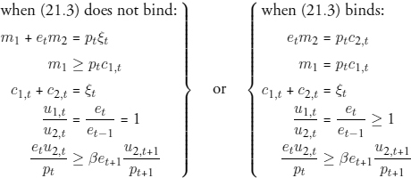
When neither melting nor minting occurs, c_1,t + c_2,t = ξ_t, and m_i,t = m_i,-1 ≡ m_i, i = 1, 2. In this case, the equilibrium conditions of the model consist of one or the other of the two following sets of inequalities, depending on whether the penny-in-advance restriction binds:

Notice that when (21.3) does not bind, there is one quantity theory equation in terms of the total stock of coins, but that when (21.3) does bind, there are two quantity theory equations, one for large purchases cast in terms of dollars, the other for small purchases in terms of the stock of pennies.

Notice also that the exchange rate e_t can only be constant or rising. It rises from t − 1 to t if there is a shortage at t. Thus, in our model, a plot of the exchange rate over time will look much like the graphs in figure 2.1.

In what follows, we begin by examining equilibria where the first set of conditions applies at all times. We will show how to construct stationary equilibria. Then we will study a variation in the endowment that brings into play the second set of inequalities, when the penny-in-advance constraint binds, all the while maintaining the requirement that neither melting nor minting occurs. Throughout, we take the mint policy (σ_i and γ_i) as fixed.

Stationary equilibria with no minting or melting

We describe a stationary equilibrium with constant monies, endowment, consumption rates, price level, and exchange rate.

Proposition 1. (A stationary, “no-shortage” equilibrium)

Assume a stationary (i.e., constant) endowment sequence ξ, and initial money stocks (m₁, m₂). Let (c₁, c₂) solve

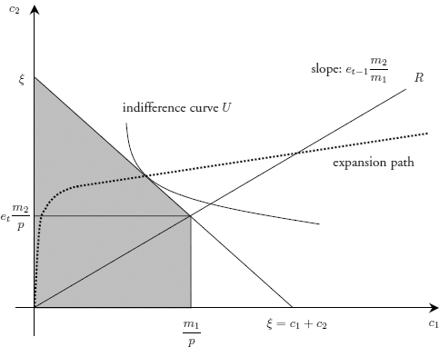
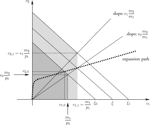
Figure 22.1 Stationary equilibrium, non-binding constraint.

Then there exists a stationary equilibrium without minting or melting if the exchange rate e satisfies the following:

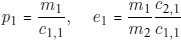
Proof: Let p = (m₁ + em₂)/ξ. By (22.4), p will satisfy (21.12) in such a way that coins are neither melted nor minted. Condition (21.2) is then satisfied with equality and (21.3) is satisfied with inequality by (22.5). Since (21.3) does not bind, θ_t = 0 and conditions (21.14) are satisfied with a constant e.

Condition (22.3), a consequence of the no-arbitrage conditions, requires that the exchange rate be set so that there exists a price level compatible with neither minting nor melting of either coin, of the type described in proposition 1. Condition (22.4) means that the total nominal quantity of money (which depends on e) is sufficient for the cash-in-advance constraint. Condition (22.5) puts an upper bound on e: the share of pennies in the nominal stock must be more than enough for the penny-in-advance constraint not to bind. Conditions (22.4) and (22.5) together imply that pc₂ ≥ em₂, that is, dollars are insufficient for large purchases.

Figure 22.1 depicts the determination of c₁, c₂, p, and satisfaction of the penny-in-advance constraint (21.3) with room to spare. There is one quantity theory equation cast in terms of the total money supply. That there is room to spare in satisfying (21.3) reveals an exchange rate indeterminacy in this setting: a range of e’s can be chosen to leave the qualitative structure of this figure intact. Notice the ray drawn with slope . So long as the endowment remains in the region where the expansion path associated with a unit relative price lies to the northwest of this ray, the penny-in-advance constraint (21.3) remains satisfied with inequality. But when movements in the endowment or in preferences put the system out of that region, it triggers a penny shortage whose character we now study.

Small coin shortages

Using the back-solving method, we display some possible patterns of endowment shifts that generate small coin shortages.

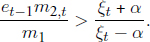
First, note that another way to interpret (22.4) and (22.5) is to take m₁, m₂, e as fixed and to formulate these conditions as bounds on ξ:

(where [22.8] is written for the logarithmic utility case). These equations reveal a variety of ways of generating small coin shortages with a change in ξ, starting from a given stationary equilibrium. The simplest, which we explore first, is a one-time change in ξ within the strict intervals defined in (22.6) and (22.7) but that violate (22.8): no minting or melting occurs, but a shortage ensues. Another way is as follows: a shortage of small change arises when the stock of pennies is insufficient relative to dollars. Suppose the lower bound in (22.6) is lower than that in (22.7). Then a shift in the endowment can lower the price level to the minting point for dollars without triggering any minting of pennies, resulting in a (relative) decrease in the penny supply; for some values of the parameters, this can violate (22.8) and generate a shortage in the period following the minting of dollars.

Small coin shortage, no minting or melting

We begin by studying the situation that arises when, following an epoch where constant money supplies and endowment were compatible with a stationary equilibrium, there occurs at time t a shift in the endowment. In figure 22.1, for the utility function v(g(c_1,t))+v(c_2,t) we drew the expansion path traced out by points where indifference curves are tangent to feasibility lines associated with different endowment levels. The expansion path is c₁ = max(0, c₂ − α), and so has slope 1 or infinity, for If i.e., if pennies compose a large enough fraction of the money stock, then the ray c₂/c₁ equaling this ratio never threatens to wander into the southeastern region described above and render (21.3) binding. However, when > 1, growth in the endowment ξ can push the economy into the southeastern region, which makes (21.3) bind and triggers an appreciation of dollars.

Thus, suppose that ξ_t is high enough that the intersection of the expansion path with the feasibility line (c₁ + c₂ = ξ_t) is below the ray e_t-1m₂/m₁. This means that at t, our second subset of equations determines prices and the allocation. If we assume that ξ_t is such that neither minting nor melting occurs (an assumption that must in the end be verified), then equilibrium values of c₁, c₂, e, p can be computed recursively as follows.

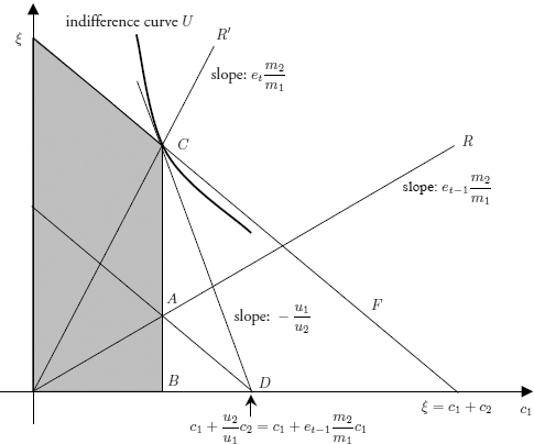
Figure 22.2 Effect of a shift in endowments.

Given e_t−1, the following three equations can be solved for c₁, c₂, e at t:

These can be combined into a single equation in c_1,t:

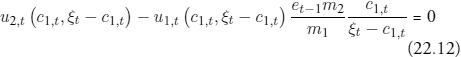
to which there exists a solution.2 Then c₂ is determined from (22.9), and e_t (which satisfies e_t > e_t-1 by construction) is given by (22.10). It remains to check that p_t = m₁/c₁ ∈ I and that the Euler inequality (21.15b) holds. There is room to satisfy the inequality if is small enough.

Figure 22.2 illustrates the situation. We use the intersections of various lines to represent the conditions (22.9), (22.10), and (22.11), and to determine the position of the consumption allocation (point C) and e_t, given e_t-1. First, the feasibility line F, on which C must lie, represents (22.9). Second, condition (22.11) means that the ray passing through point C has slope e_tm₂/m₁: this defines e_t.

Finally, condition (22.10) relates the rate of return on large coins (the slope of R compared to the slope of R') with the slope of the indifference curve at C. To represent this geometrically, (22.11) can be used to transform (22.10) into the following:

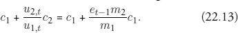
Define point A to be the vertical projection of C onto the ray e_t-1m₂/m₁. The right-hand side of (22.13) is the point at which a line, parallel to the feasibility line and drawn through point A, intersects the x-axis. The left-hand side is the point where the tangent to the indifference curve at C intersects the x-axis. Condition (22.10) requires that these intersections coincide. When they do, the segments AB and BD have same length (because AD has slope − 1), and therefore the ratios CB/BD and CB/AB are equal. The former is the slope of the indifference curve at C, and the latter is the ratio of the slopes of R' and R, in other words the rate of return of large coins relative to small coins.

Permanent and transitory increases in ξ

Having determined the new exchange rate e_t after a shift in the endowment ξ_t, we can determine what happens if the shift is permanent or transitory. If it is permanent, then the constraint (21.3) will continue to bind. The reason is that, since e_t > e_t-1, the ray e_tm₂/m₁ is in fact even higher than e_t-1m₂/m₁, which means that the expansion path remains below the ray, and the penny constraint continues to bind. This situation cannot continue indefinitely without minting or melting, however. Thus, a permanent upward shift in the endowment from the situation depicted in figure 22.1 to that in figure 22.2 would impel a sequence of increases in the exchange rate until eventually the price level is pushed outside the interval I.

As for a temporary (one-time) increase in ξ_t, it might prompt further increases in the exchange rate even if the endowment immediately subsides to its original level. The reason is that the increase in e induces a permanent upward shift in the ray that enlarges the southeastern region where (21.3) is binding.

Logarithmic example

We can go further in analyzing the results of shifts of endowments by supposing that v(.) = ln(.) in equation(21.1). For this specification we can compute solutions by hand.

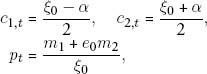
Consider a steady state with constant ξ_t = ξ0, m₁, m₂, and e_t = e₀, such that the constraint (21.3) does not bind. The equilibrium objects are

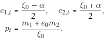
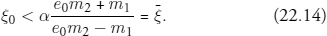
The condition that ξ₀, m₁, m₂ and e₀ must satisfy for (21.3) not to bind is:

The income level corresponds to the intersection of the expansion path and the ray e₀m₂/m₁ in figure 22.1.

Suppose that, at t = 1, ξ increases above so that (22.14) is violated. Then e₀ cannot be the exchange rate at t = 1 and (21.3) binds at t = 1. The equilibrium objects at t = 1 become:

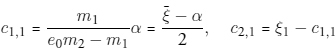
Figure 22.3 Effect of a shift in endowments (logarithmic case).

It can be shown that p₁/p₀ = ξ₀/; so that the price level initially falls at t = 1, although to a level independent of ξ₁. (It must be checked that p₁ is not so low as to reach one of the minting points, since we are assuming throughout that m₁ and m₂ do not change.) Consumption c₁ is also unrelated to ξ₁, and is limited to the amount that would be consumed at the income level , just where the constraint begins to bind.

Figure 22.3 illustrates the effect of a shift in the endowment from ξ₀ to ξ₁ > . The corner in the new budget set (light shade) is vertically aligned with the intersection of the expansion path and the ray e₀m₂/m₁. The position of that corner also determines the new exchange rate, since the ray going through that corner has slope e₁m₂/m₁. It is also apparent from the graph that p₁ is lower than p₀ (because m₁/p₁ is greater than m₁/p₀) and that it has the same value for all ξ₁ ≥ . The exchange rate e₁, however, is increasing in ξ₁

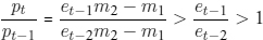
Consider now the case where ξ remains fixed at ξ₁ permanently after t = 1. The penny-in-advance constraint continues to bind, implying that the exchange rate continues to increase. In every period, the ray e_t(m₂/m₁) moves up, and c_1,t = m₁/(e_t-1m₂ − m₁) falls, moving further away from the first-best allocation and indicating that the shortage of small change becomes increasingly severe. Furthermore, the price level p_t = m₁/c_1,t now rises, and the rate of inflation is that is, the price level rises faster than the exchange rate did the previous period.

Suppose now that, after jumping from ξ₀ to ξ₁, income falls back to its earlier value ξ₀ and stays there. If ξ₁ was large enough (specifically, if ξ₁ > (c_1,1/c_1,0)ξ₀), then the ray e₁(m₂/m₁) has moved high enough that the expansion path is in the southeastern region, as depicted in figure 22.3. In that case, the shortage will continue, and e_t will continue to increase as in the case of a permanent change ξ.

Money shortages bring inflation

If we return to the supply side as shown in figure 21.1, we see that the price level initially fell. It might fall enough to reach the minting point for dollars, in which case the shortage is worsened, as we will see shortly. Assuming as we did that p₁ did not reach either minting point, the shortage continues, and e_t rises, which shifts the lower interval to the right at a “speed” e_t/e_t-1. But the price level now moves to the right as well, and at an even higher speed. This suggests that the price level will reach the melting point for either dollars or pennies before it is caught up by the minting point for dollars. If pennies are melted, the shortage is aggravated further.

The two forms of inflation, in e_t and in p_t, are linked because the quantity theory equation has split into two separate, albeit related components e_tm₂ = p_tc₂,_t and m₁ = p_tc₁,_t. The link is subtle because the quantities c₁ and c₂ are changing as well.

An enduring shortage of small change without minting or melting leads to the paradoxical situation of sustained inflation in the absence of any change in the stock of money. Stranger still, it is the shortage of (one type of) money that causes the general inflation. Ultimately, the price level is bounded by γ₁, the melting point for pennies. If pennies were initially light, then γ₁ could be substantially above the initial price level, and the shortage-induced inflation could be significant.

Shortages of small coins through minting of large coins

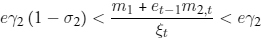
A shortage of small coins can also occur as a consequence of minting, independently of the “income effect” we have described. Assume that all coins are full-bodied, so that the bounds of the intervals coincide to the right (γ₁ = eγ₂), but that production costs require that a higher seigniorage be levied on small coins (σ₁ > σ₂), so that the left boundaries do not coincide (γ₁(1 − σ₁) < eγ₂(1 − σ₂)).

In the previous section, we considered “small” increases in the endowment ξ; that is, increases that led to movements in the price level p_t within the intervals dictated by the arbitrage conditions. We now consider “large” increases that will induce such a fall in the price level that it reaches the minting point for large coins (p_t = eγ₂(1 − σ₂)). The structure of coin specifications and minting charges means that small coins will not be minted. As a result, m₂ increases while m₁ remains unchanged, and the ratio em₂/m₁ rises. The intuition garnered from figure 22.2 suggests that, for large enough increases in m2, trouble may occur; a shortage of small change results, because the share of pennies in the total money stock falls too far. We verify that this can indeed happen.

We begin again from a stationary equilibrium with no minting or melting. Suppose that, at time t, the endowment increases from ξ₀ to ξ_t, with the latter satisfying ξ_t > (m₁ + em₂)/eγ₂(1 − σ₂) so as to violate (22.7). Then minting occurs at t, and the price level is known: p_t = eγ₂(1 − σ₂).

As before, two situations can arise, depending on whether (21.3) is binding or not at t. We will look for equilibria where it is not. Then u₂ = u₁, which, combined with the binding cash-in-advance constraint (21.2), allows to solve for c_1,t and c_2,t. Now we know the amount minted, namely, ξ_t − c_1,t − c_2,t (positive by assumption), and the addition to the money stock is n_2t = γ₂(ξ_t − c_1,t − c_2,t).

At t + 1, it can be shown that

or, in other words, that no more minting occurs if (21.3) does not bind. But (21.3) binds if the following holds:

At equality, this becomes a second-degree polynomial in ξ_t, which, for large enough values of ξ_t, will have a positive root. Thus, if enough dollars are minted, pennies become relatively short of supply.

Shortages through melting of full-weight small coins

In this section, we modify the model to include underweight small denomination coins. The modifications are designed to capture the circumstances that prevailed in England around 1695, described in chapter 16. In this case, an initial shortage of small coins leads to melting of some of the small coins, as well as minting of large coins.

We make two modifications. One is to assume that σ₁ = σ₂ = 0, which was true in England in the 1690s. The other is to introduce underweight coins, as described above. Specifically, we assume that, at t = 0, the stock of small coins is divided between full-weight coins and underweight coins, weighing a fraction δ of the full-weight coins. We assume that the stock of underweight coins is inherited from the past, and for simplicity we do not model the creation of underweight coins.3 As described on page 346, the existence of underweight coins creates two melting points, one for full-weight coins at γ₁ and another for underweight coins at γ₁/δ.⁴

We consider an experiment in which an initial steady state prevails with the penny-in-advance constraint (21.3) not binding, followed by an increase in income at t = 1 that makes the constraint binding. As above, in the logarithmic case, the initial equilibrium values are with e₀ = γ₁/γ₂ and p₀ = γ₁ = e₀γ₂.

At t = 1, income is ξ₁ > and the penny-in-advance constraint binds. It follows that e₁ > e₀. Since the no-arbitrage conditions impose p₁ ≥ e₁γ₂, the price level rises and p₁ > γ₁. This implies that all full-weight small denomination coins are melted. Assume that p₁ < γ₁/α so that no underweight small denomination coins are melted.

Although minting and melting take place at t = 1, quantities c_1,1 and c_2,1 are determined by the incoming stocks of money m_1,0 and m_2,0, along with the new price level p1, via the two quantity theory equations.

The quantity theory equations p₁c_1,1 = e₁m_2,0 imply

This, along with (21.17), gives

while feasibility gives

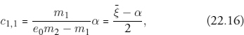
Equations (22.17) and (22.15) allow us to solve for the change in the stock of large coins µ_2,1 − n_2,1 as a function of c_1,1, which is known from (22.16). One finds

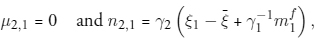
which means that the stock of large coins increases, and by more than the stock of small coin decreases. Finally, one finds c_2,1 = ( + α)/2.

Our model thus predicts the following symptoms of a small coin shortage: the heavier small coins will be melted or exported, coinage of the large coins will increase substantially, prices will rise and so will the exchange rate between large and small coins. All of these symptoms were present in the second half of 1695, as we saw in chapter 16.

Consider now the new ray e₁(m_2,1/m_1,1) and note that, from t = 0 to t = 1, e and m₂ have increased while m₁ has fallen. As a result, the ray is now higher than before. The shortage situation is thus likely to persist, whether the change in income ξ is permanent or transitory.

The opposing policies of Lowndes and Locke can readily be formulated in terms of the model. Lowndes advocated a debasement so that γ₁ becomes γ₁ = p₁ = e₁γ₂. He argued for an increase in the supply of small coins (if necessary by subsidizing the mint) and claimed that it would not be inflationary. In our model, Lowndes is correct: if it were of the proper amount, such an increase in m₁ would not be inflationary because it would relax the constraint on consumption of small goods.

In 1695, the government of England decided to remint at its expense, at the old standard: that is, the mint was ordered to melt µ₁ = into αb₁ ounces of silver, and to make at the old standard b₁ the quantity of coins . The net result would be to decrease the stock of small coins m₁ by a fraction 1 − α, the cost borne by the taxpayer.

Perverse effects and their palliatives

We have thus shown two ways that endowment growth can induce small coin shortages, with or without minting. We now discuss how such episodes affect the monetary system over time, in particular the relation between small and large coins.

A shortage of small coins manifests itself in a binding penny-in-advance constraint (21.3), and is associated with two kinds of price adjustments, one “static,” the other “dynamic.” First, the quantity theory breaks into two separate equations, one for small, another for large coins taking the forms p_t = m_1,t/c_1,t and e_t = . The mitosis of the quantity theory is the time-t consequence of a shortage of small coins. A second response is dynamic, and requires that e_t > e_t-1, so that dollars appreciate with respect to the pennies. This response equilibrates the demand side but has perverse implications because of its eventual effects on supply. For fixed b₂, an increase in e shifts the interval [e(1 − σ₂)γ₂,eγ₂] to the right, leaving the interval [(1 − σ₁)γ₁,γ₁] fixed. This reduces the intersection I and hastens the occasion when either more dollars will be minted or pennies will be melted, depending on which bound the price level hits first. Thus, shortages of small coins ultimately reduce their supply, relatively or even absolutely, a perverse outcome.

This penny-impoverishing implication of a rise in e induced by a shortage isolates a force for the government to adopt a commensurate reduction in b₁. This shifts the penny interval in line with the dollar interval, eventually resupplying the system with a new, lighter penny. Sargent and Smith’s (1997) analysis of a noninflationary debasement in a one-coin system can be adapted to simulate such a debasement. ⁵

An alternative way to realign the two intervals in response to a shortage-induced increase in e would be to raise b₂, thereby counteracting the rightward shift of the dollar interval. A shortage-induced debasement of small coins and a “reinforcement” of large coins have different implications for the price level in terms of pence: the former lets it rise with e, the latter stabilizes it. The price level in terms of dollars would remain constant with the former, fall with the latter. In a world with nominal debt contracts, the two policies have different implications for debtors and creditors.

Parts III and IV cited many examples of historical shortages of small change that we interpreted in terms of the theoretical shortages that can emerge in our model. The following chapter describes how some remedies for shortages, such as the standard formula, work in our model.

---

¹ See Sims (1989, 1990) and Díaz-Giménez et al. (1992).

² Call f(c_1,t) the left-hand side of (22.12). Since the expansion path intersects the feasibility line above the ray e_–1m₂/m₁, the coordinates of that intersection (c₁, ξ − c₁) satisfy f(c₁) < 0. Also, lim_c1→0 f(c₁) = u₂(0,ξ)>0.

³ See Sargent and Smith (1997) for a simple model of physical depreciation of coins.

⁴ Feavearyear (1963, 123) cited evidence that underweight coins were more likely to be counterfeited in England: “Meanwhile its (the Mint’s) workmen made copies of the old clipped groats, and issued them, at a good profit, to people who apparently accepted them freely and used them. Nobody troubled to counterfeit milled money, for there was no profit in it.”

⁵ This experiment stresses the extent to which a “circulation by tale” axiom is embedded in our framework: for the purposes of the cash-in-advance constraint (21.3), a penny is a penny, whatever its weight. To analyze a debasement as described in the text, one has to keep track of two kinds of pennies, old and new.