To illustrate the present value formula, consider a simple bond that matures in four years, has a coupon rate of 10%, and has a maturity value of $100. For simplicity, let’s assume the bond pays interest annually and a discount rate of 8% should be used to calculate the present value of each cash flow. The cash flow for this bond is:

Year	Cash flow
1	$10
2	10
3	10
4	110

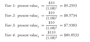
The present value of each cash flow is:

The value of this security is then the sum of the present values of the four cash flows. That is, the present value is $106.6243 ($9.2593 + $8.5734 + $7.9383 + $80.8533).

1. Present Value Properties An important property about the present value can be seen from the above illustration. For the first three years, the cash flow is the same ($10) and the discount rate is the same (8%). The present value decreases as we go further into the future. This is an important property of the present value: for a given discount rate, the further into the future a cash flow is received, the lower its present value. This can be seen in the present value formula. As t increases, present value_t decreases.

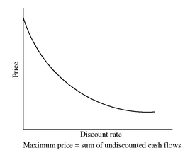
EXHIBIT 1 Price/Discount Rate Relationship for an Option-Free Bond

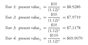
Suppose that instead of a discount rate of 8%, a 12% discount rate is used for each cash flow. Then, the present value of each cash flow is:

The value of this security is then $93.9253 ($8.9286 + $7.9719 + $7.1178 + $69.9070). The security’s value is lower if a 12% discount rate is used compared to an 8% discount rate ($93.9253 versus $106.6243). This is another general property of present value: the higher the discount rate, the lower the present value. Since the value of a security is the present value of the expected cash flows, this property carries over to the value of a security: the higher the discount rate, the lower a security’s value. The reverse is also true: the lower the discount rate, the higher a security’s value.

Exhibit 1 shows, for an option-free bond, this inverse relationship between a security’s value and the discount rate. The shape of the curve in Exhibit 1 is referred to as convex. By convex, it is meant the curve is bowed in from the origin. As we will see in Chapter 7, this convexity or bowed shape has implications for the price volatility of a bond when interest rates change. What is important to understand is that the relationship is not linear.

2. Relationship between Coupon Rate, Discount Rate, and Price Relative to Par Value In Chapter 2, we described the relationship between a bond’s coupon rate, required market yield, and price relative to its par value (i.e., premium, discount, or equal to par). The required yield is equivalent to the discount rate discussed above. We stated the following relationship:

coupon rate = yield required by market, therefore price = par value
coupon rate < yield required by market, therefore price < par value (discount)
coupon rate > yield required by market, therefore price > par value (premium)

Now that we know how to value a bond, we can demonstrate the relationship. The coupon rate on our hypothetical bond is 10%. When an 8% discount rate is used, the bond’s value is $106.6243. That is, the price is greater than par value (premium). This is because the coupon rate (10%) is greater than the required yield (the 8% discount rate). We also showed that when the discount rate is 12% (i.e., greater than the coupon rate of 10%), the price of the bond is $93.9253. That is, the bond’s value is less than par value when the coupon rate is less than the required yield (discount). When the discount rate is the same as the coupon rate, 10%, the bond’s value is equal to par value as shown below:

Year	Cash flow	Present value at 10%
1	$10	$9.0909
2	10	8.2645
3	10	7.5131
4	110	75.1315
	Total	$100.0000

3. Change in a Bond’s Value as it Moves Toward Maturity As a bond moves closer to its maturity date, its value changes. More specifically, assuming that the discount rate does not change, a bond’s value:

1. decreases over time if the bond is selling at a premium

2. increases over time if the bond is selling at a discount

3. is unchanged if the bond is selling at par value

At the maturity date, the bond’s value is equal to its par value. So, over time as the bond moves toward its maturity date, its price will move to its par value—a characteristic sometimes referred to as a “pull to par value.”

To illustrate what happens to a bond selling at a premium, consider once again the 4-year 10% coupon bond. When the discount rate is 8%, the bond’s price is 106.6243. Suppose that one year later, the discount rate is still 8%. There are only three cash flows remaining since the bond is now a 3-year security. The cash flow and the present value of the cash flows are given below:

Year	Cash flow	Present value at 8%
1	$10	$9.2593
2	10	8.5734
3	110	87.3215
	Total	$105.1542

The price has declined from $106.6243 to $105.1542.

Now suppose that the bond’s price is initially below par value. For example, as stated earlier, if the discount rate is 12%, the 4-year 10% coupon bond’s value is $93.9253. Assuming the discount rate remains at 12%, one year later the cash flow and the present value of the cash flow would be as shown:

Year	Cash flow	Present value at 12%
1	$10	$8.9286
2	10	7.9719
3	110	78.2958
	Total	$95.1963

The bond’s price increases from $93.9253 to $95.1963.

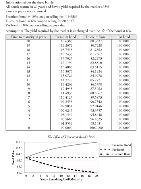
To understand how the price of a bond changes as it moves towards maturity, consider the following three 20-year bonds for which the yield required by the market is 8%: a premium bond (10% coupon), a discount bond (6% coupon), and a par bond (8% coupon).To simplify the example, it is assumed that each bond pays interest annually. Exhibit 2 shows the price of each bond as it moves toward maturity, assuming that the 8% yield required by the market does not change. The premium bond with an initial price of 119.6363 decreases in price until it reaches par value at the maturity date. The discount bond with an initial price of 80.3637 increases in price until it reaches par value at the maturity date.

In practice, over time the discount rate will change. So, the bond’s value will change due to both the change in the discount rate and the change in the cash flow as the bond moves toward maturity. For example, again suppose that the discount rate for the 4-year 10% coupon is 8% so that the bond is selling for $106.6243. One year later, suppose that the discount rate appropriate for a 3-year 10% coupon bond increases from 8% to 9%. Then the cash flow and present value of the cash flows are shown below:

Year	Cash flow	Present value at 9%
1	$10	$9.1743
2	10	8.4168
3	110	84.9402
	Total	$102.5313

The bond’s price will decline from $106.6243 to $102.5313. As shown earlier, if the discount rate did not increase, the price would have declined to only $105.1542. The price decline of $4.0930 ($106.6243 − $102.5313) can be decomposed as follows:

D. Valuation Using Multiple Discount Rates

Thus far, we have used one discount rate to compute the present value of each cash flow. As we will see shortly, the proper way to value the cash flows of a bond is to use a different discount rate that is unique to the time period in which a cash flow will be received. So, let’s look at how we would value a security using a different discount rate for each cash flow.

Suppose that the appropriate discount rates are as follows:

year 1	6.8%
year 2	7.2%
year 3	7.6%
year 4	8.0%

EXHIBIT 2 Movement of a Premium, Discount, and Par Bond as a Bond Moves Towards Maturity

Then, for the 4-year 10% coupon bond, the present value of each cash flow is:

The present value of this security, assuming the above set of discount rates, is $106.9456.

E. Valuing Semiannual Cash Flows

In our illustrations, we assumed coupon payments are paid once per year. For most bonds, the coupon payments are semiannual. This does not introduce any complexities into the calculation. The procedure is to simply adjust the coupon payments by dividing the annual coupon payment by 2 and adjust the discount rate by dividing the annual discount rate by 2. The time period t in the present value formula is treated in terms of 6-month periods rather than years.

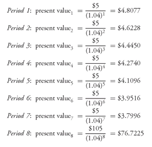
For example, consider once again the 4-year 10% coupon bond with a maturity value of $100. The cash flow for the first 3.5 years is equal to $5 ($10/2). The last cash flow is equal to the final coupon payment ($5) plus the maturity value ($100). So the last cash flow is $105.

Now the tricky part. If an annual discount rate of 8% is used, how do we obtain the semiannual discount rate? We will simply use one-half the annual rate, 4% (or 8%/2). The reader should have a problem with this: a 4% semiannual rate is not an 8% effective annual rate. That is correct. However, as we will see in the next chapter, the convention in the bond market is to quote annual interest rates that are just double semiannual rates. This will be explained more fully in the next chapter. Don’t let this throw you off here. For now, just accept the fact that one-half an annual discount rate is used to obtain a semiannual discount rate in the balance of the chapter.

Given the cash flows and the semiannual discount rate of 4%, the present value of each cash flow is shown below:

The security’s value is equal to the sum of the present value of the eight cash flows, $106.7327. Notice that this price is greater than the price when coupon payments are annual ($106.6243). This is because one-half the annual coupon payment is received six months sooner than when payments are annual. This produces a higher present value for the semiannual coupon payments relative to the annual coupon payments.

The value of a non-amortizing bond can be divided into two components: (1) the present value of the coupon payments and (2) the present value of the maturity value. For a fixed-rate coupon bond, the coupon payments represent an annuity. A short-cut formula can be used to compute the value of a bond when using a single discount rate: compute the present value of the annuity and then add the present value of the maturity value.⁴⁷

The present value of an annuity is equal to:

For a bond with annual interest payments, i is the annual discount rate and the “no. of periods” is equal to the number of years.

Applying this formula to a semiannual-pay bond, the annuity payment is one half the annual coupon payment and the number of periods is double the number of years to maturity. So, the present value of the coupon payments can be expressed as:

where i is the semiannual discount rate (annual rate/2). Notice that in the formula, we use the number of years multiplied by 2 since a period in our illustration is six months.

The present value of the maturity value is equal to

To illustrate this computation, consider once again the 4-year 10% coupon bond with an annual discount rate of 8% and a semiannual discount rate of one half this rate (4%) for the reason cited earlier. Then:

semiannual coupon payment	= $5
semiannual discount rate(i)	= 4%
number of years	= 4

then the present value of the coupon payments is

To determine the price, the present value of the maturity value must be added to the present value of the coupon payments. The present value of the maturity value is

The price is then $106.7327 ($33.6637 + $73.0690). This agrees with our previous calculation for the price of this bond.

F. Valuing a Zero-Coupon Bond

For a zero-coupon bond, there is only one cash flow—the maturity value. The value of a zero-coupon bond that matures N years from now is

where i is the semiannual discount rate.

It may seem surprising that the number of periods is double the number of years to maturity. In computing the value of a zero-coupon bond, the number of 6-month periods (i.e., “no. of years ×2”) is used in the denominator of the formula. The rationale is that the pricing of a zero-coupon bond should be consistent with the pricing of a semiannual coupon bond. Therefore, the use of 6-month periods is required in order to have uniformity between the present value calculations.

To illustrate the application of the formula, the value of a 5-year zero-coupon bond with a maturity value of $100 discounted at an 8% interest rate is $67.5564, as shown below:

G. Valuing a Bond Between Coupon Payments

For coupon-paying bonds, a complication arises when we try to price a bond between coupon payments. The amount that the buyer pays the seller in such cases is the present value of the cash flow. But one of the cash flows, the very next cash flow, encompasses two components as shown below:

1. interest earned by the seller

2. interest earned by the buyer

The interest earned by the seller is the interest that has accrued⁴⁸ between the last coupon payment date and the settlement date.⁴⁹ This interest is called accrued interest. At the time of purchase, the buyer must compensate the seller for the accrued interest. The buyer recovers the accrued interest when the next coupon payment is received.

When the price of a bond is computed using the present value calculations described earlier, it is computed with accrued interest embodied in the price. This price is referred to as the full price. (Some market participants refer to it as the dirty price.) It is the full price that the buyer pays the seller. From the full price, the accrued interest must be deducted to determine the price of the bond, sometimes referred to as the clean price.

Below, we show how the present value formula is modified to compute the full price when a bond is purchased between coupon periods.

1. Computing the Full Price To compute the full price, it is first necessary to determine the fractional periods between the settlement date and the next coupon payment date. This is determined as follows:

Then the present value of the expected cash flow to be received t periods from now using a discount rate i assuming the first coupon payment is w periods from now is:

This procedure for calculating the present value when a security is purchased between coupon payments is called the “Street method.”

To illustrate the calculation, suppose that there are five semiannual coupon payments remaining for a 10% coupon bond. Also assume the following:

1. 78 days between the settlement date and the next coupon payment date

2. 182 days in the coupon period

Then w is 0.4286 periods (= 78/182). The present value of each cash flow assuming that each is discounted at 8% annual discount rate is

The full price is the sum of the present value of the cash flows, which is $106.8192. Remember that the full price includes the accrued interest that the buyer is paying the seller.

2. Computing the Accrued Interest and the Clean Price To find the price without accrued interest, called the clean price or simply price, the accrued interest must be computed. To determine the accrued interest, it is first necessary to determine the number of days in the accrued interest period. The number of days in the accrued interest period is determined as follows:

days in accrued interest period =
days in coupon period − days between settlement and next coupon payment

The percentage of the next semiannual coupon payment that the seller has earned as accrued interest is found as follows:

So, for example, returning to our illustration where the full price was computed, since there are 182 days in the coupon period and there are 78 days from the settlement date to the next coupon payment, the days in the accrued interest period is 182 minus 78, or 104 days. Therefore, the percentage of the coupon payment that is accrued interest is:

This is the same percentage found by simply subtracting w from 1. In our illustration, w was 0.4286. Then 1 − 0.4286 = 0.5714.

Given the value of w, the amount of accrued interest (AI) is equal to:

AI = semiannual coupon payment × (1 − w)

So, for the 10% coupon bond whose full price we computed, since the semiannual coupon payment per $100 of par value is $5 and w is 0.4286, the accrued interest is:

$5 × (1 − 0.4286) = $2.8570

The clean price is then:

full price − accrued interest

In our illustration, the clean price is⁵⁰

$106.8192 − $2.8570 = $103.9622

3. Day Count Conventions The practice for calculating the number of days between two dates depends on day count conventions used in the bond market. The convention differs by the type of security. Day count conventions are also used to calculate the number of days in the numerator and denominator of the ratio w.

The accrued interest (AI) assuming semiannual payments is calculated as follows:

In calculating the number of days between two dates, the actual number of days is not always the same as the number of days that should be used in the accrued interest formula. The number of days used depends on the day count convention for the particular security. Specifically, day count conventions differ for Treasury securities and government agency securities, municipal bonds, and corporate bonds.

For coupon-bearing Treasury securities, the day count convention used is to determine the actual number of days between two dates. This is referred to as the “actual/actual” day count convention. For example, consider a coupon-bearing Treasury security whose previous coupon payment was March 1. The next coupon payment would be on September 1. Suppose this Treasury security is purchased with a settlement date of July 17th. The actual number of days between July 17 (the settlement date) and September 1 (the date of the next coupon payment) is 46 days, as shown below:

July 17 to July 31	14 days
August	31 days
September 1	1 day
	46 days

Note that the settlement date (July 17) is not counted. The number of days in the coupon period is the actual number of days between March 1 and September 1, which is 184 days. The number of days between the last coupon payment (March 1) through July 17 is therefore 138 days (184 days − 46 days).

For coupon-bearing agency, municipal, and corporate bonds, a different day count convention is used. It is assumed that every month has 30 days, that any 6-month period has 180 days, and that there are 360 days in a year. This day count convention is referred to as “30/360.” For example, consider once again the Treasury security purchased with a settlement date of July 17, the previous coupon payment on March 1, and the next coupon payment on September 1. If the security is an agency, municipal, or corporate bond, the number of days until the next coupon payment is 44 days as shown below:

July 17 to July 31	13 days
August	30 days
September 1	1 day
	44 days

Note that the settlement date, July 17, is not counted. Since July is treated as having 30 days, there are 13 days (30 days minus the first 17 days in July). The number of days from March 1 to July 17 is 136, which is the number of days in the accrued interest period.

III. TRADITIONAL APPROACH TO VALUATION

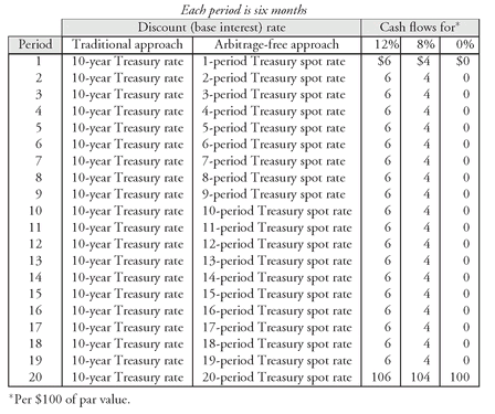
The traditional approach to valuation has been to discount every cash flow of a fixed income security by the same interest rate (or discount rate). For example, consider the three hypothetical 10-year Treasury securities shown in Exhibit 3: a 12% coupon bond, an 8% coupon bond, and a zero-coupon bond. The cash flows for each bond are shown in the exhibit. Since the cash flows of all three bonds are viewed as default free, the traditional practice is to use the same discount rate to calculate the present value of all three bonds and use the same discount rate for the cash flow for each period. The discount rate used is the yield for the on-the-run issue obtained from the Treasury yield curve. For example, suppose that the yield for the 10-year on-the-run Treasury issue is 10%. Then, the practice is to discount each cash flow for each bond using a 10% discount rate.

EXHIBIT 3 Cash Flows for Three 10-Year Hypothetical Treasury Securities Per $100 of Par Value

	Coupon rate
Each period is six months
Period	12%	8%	0%
1 - 19	$6	$4	$0
20	106	104	100

For a non-Treasury security, a yield premium or yield spread is added to the on-the-run Treasury yield. The yield spread is the same regardless of when a cash flow is to be received in the traditional approach. For a 10-year non-Treasury security, suppose that 90 basis points is the appropriate yield spread. Then all cash flows would be discounted at the yield for the on-the-run 10-year Treasury issue of 10% plus 90 basis points.

IV. THE ARBITRAGE-FREE VALUATION APPROACH

The fundamental flaw of the traditional approach is that it views each security as the same package of cash flows. For example, consider a 10-year U.S. Treasury issue with an 8% coupon rate. The cash flows per $100 of par value would be 19 payments of $4 every six months and $104 twenty 6-month periods from now. The traditional practice would discount each cash flow using the same discount rate.

The proper way to view the 10-year 8% coupon Treasury issue is as a package of zero-coupon bonds whose maturity value is equal to the amount of the cash flow and whose maturity date is equal to each cash flow’s payment date. Thus, the 10-year 8% coupon Treasury issue should be viewed as 20 zero-coupon bonds. The reason this is the proper way to value a security is that it does not allow arbitrage profit by taking apart or “stripping” a security and selling off the stripped securities at a higher aggregate value than it would cost to purchase the security in the market. We’ll illustrate this later. We refer to this approach to valuation as the arbitrage-free valuation approach.⁵¹

EXHIBIT 4 Comparison of Traditional Approach and Arbitrage-Free Approach in Valuing a Treasury Security

By viewing any financial asset as a package of zero-coupon bonds, a consistent valuation framework can be developed. Viewing a financial asset as a package of zero-coupon bonds means that any two bonds would be viewed as different packages of zero-coupon bonds and valued accordingly.

The difference between the traditional valuation approach and the arbitrage-free approach is illustrated in Exhibit 4, which shows how the three bonds whose cash flows are depicted in Exhibit 3 should be valued. With the traditional approach, the discount rate for all three bonds is the yield on a 10-year U.S. Treasury security. With the arbitrage-free approach, the discount rate for a cash flow is the theoretical rate that the U.S. Treasury would have to pay if it issued a zero-coupon bond with a maturity date equal to the maturity date of the cash flow.

Therefore, to implement the arbitrage-free approach, it is necessary to determine the theoretical rate that the U.S. Treasury would have to pay on a zero-coupon Treasury security for each maturity. As explained in the previous chapter, the name given to the zero-coupon Treasury rate is the Treasury spot rate. In Chapter 6, we will explain how the Treasury spot rate can be calculated. The spot rate for a Treasury security is the interest rate that should be used to discount a default-free cash flow with the same maturity. We call the value of a bond based on spot rates the arbitrage-free value.

EXHIBIT 5 Determination of the Arbitrage-Free Value of an 8% 10-year Treasury

A. Valuation Using Treasury Spot Rates

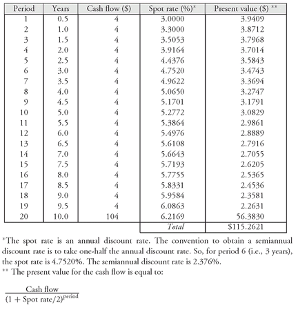
For the purposes of our discussion, we will take the Treasury spot rate for each maturity as given. To illustrate how Treasury spot rates are used to compute the arbitrage-free value of a Treasury security, we will use the hypothetical Treasury spot rates shown in the fourth column of Exhibit 5 to value an 8% 10-year Treasury security. The present value of each period’s cash flow is shown in the last column. The sum of the present values is the arbitrage-free value for the Treasury security. For the 8% 10-year Treasury, it is $115.2619.

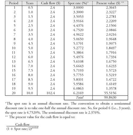
As a second illustration, suppose that a 4.8% coupon 10-year Treasury bond is being valued based on the Treasury spot rates shown in Exhibit 5. The arbitrage-free value of this bond is $90.8428 as shown in Exhibit 6.

In the next chapter, we discuss yield measures. The yield to maturity is a measure that would be computed for this bond. We won’t show how it is computed in this chapter, but simply state the result. The yield for the 4.8% coupon 10-year Treasury bond is 6.033%. Notice that the spot rates are used to obtain the price and the price is then used to compute a conventional yield measure. It is important to understand that there are an infinite number of spot rate curves that can generate the same price of $90.8428 and therefore the same yield. (We return to this point in the next chapter.)

EXHIBIT 6 Determination of the Arbitrage-Free Value of a 4.8% 10-year Treasury

B. Reason for Using Treasury Spot Rates

Thus far, we simply asserted that the value of a Treasury security should be based on discounting each cash flow using the corresponding Treasury spot rate. But what if market participants value a security using the yield for the on-the-run Treasury with a maturity equal to the maturity of the Treasury security being valued? (In other words, what if participants use the yield on coupon-bearing securities rather than the yield on zero-coupon securities?) Let’s see why a Treasury security will have to trade close to its arbitrage-free value.

1. Stripping and the Arbitrage-Free Valuation The key in the process is the existence of the Treasury strips market. As explained in Chapter 3, a dealer has the ability to take apart the cash flows of a Treasury coupon security (i.e., strip the security) and create zero-coupon securities. These zero-coupon securities, which we called Treasury strips, can be sold to investors. At what interest rate or yield can these Treasury strips be sold to investors? They can be sold at the Treasury spot rates. If the market price of a Treasury security is less than its value using the arbitrage-free valuation approach, then a dealer can buy the Treasury security, strip it, and sell off the Treasury strips so as to generate greater proceeds than the cost of purchasing the Treasury security. The resulting profit is an arbitrage profit. Since, as we will see, the value determined by using the Treasury spot rates does not allow for the generation of an arbitrage profit, this is the reason why the approach is referred to as an “arbitrage-free” approach.

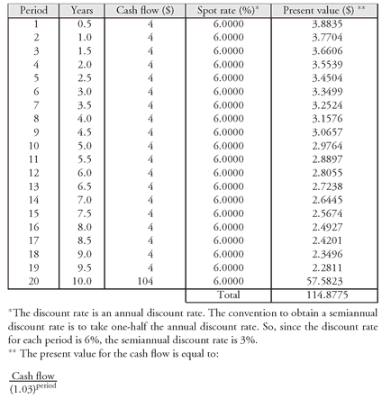
To illustrate this, suppose that the yield for the on-the-run 10-year Treasury issue is 6%. (We will see in Chapter 6 that the Treasury spot rate curve in Exhibit 5 was generated from a yield curve where the on-the-run 10-year Treasury issue was 6%.) Suppose that the 8% coupon 10-year Treasury issue is valued using the traditional approach based on 6%. Exhibit 7 shows the value based on discounting all the cash flows at 6% is $114.8775.

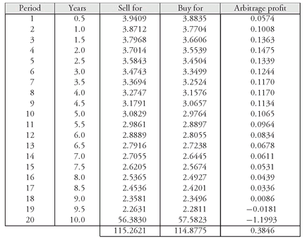
Consider what would happen if the market priced the security at $114.8775. The value based on the Treasury spot rates (Exhibit 5) is $115.2621. What can the dealer do? The dealer can buy the 8% 10-year issue for $114.8775, strip it, and sell the Treasury strips at the spot rates shown in Exhibit 5. By doing so, the proceeds that will be received by the dealer are $115.2621. This results in an arbitrage profit of $0.3846 (= $115.2621 − $114.8775).⁵² Dealers recognizing this arbitrage opportunity will bid up the price of the 8% 10-year Treasury issue in order to acquire it and strip it. At what point will the arbitrage profit disappear? When the security is priced at $115.2621, the value that we said is the arbitrage-free value.

To understand in more detail where this arbitrage profit is coming from, look at Exhibit 8.The third column shows how much each cash flow can be sold for by the dealer if it is stripped. The values in the third column are simply the present values in Exhibit 5 based on discounting the cash flows at the Treasury spot rates. The fourth column shows how much the dealer is effectively purchasing the cash flow if each cash flow is discounted at 6%. This is the last column in Exhibit 7. The sum of the arbitrage profit from each cash flow stripped is the total arbitrage profit.

2. Reconstitution and Arbitrage-Free Valuation We have just demonstrated how coupon stripping of a Treasury issue will force its market value to be close to the value determined by arbitrage-free valuation when the market price is less than the arbitrage-free value. What happens when a Treasury issue’s market price is greater than the arbitrage-free value? Obviously, a dealer will not want to strip the Treasury issue since the proceeds generated from stripping will be less than the cost of purchasing the issue.

When such situations occur, the dealer will follow a procedure called reconstitution.⁵³ Basically, the dealer can purchase a package of Treasury strips so as to create a synthetic (i.e., artificial) Treasury coupon security that is worth more than the same maturity and same coupon Treasury issue.

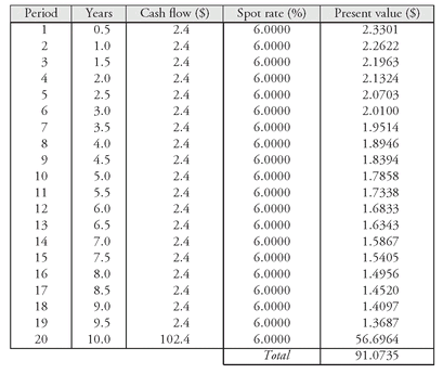
To illustrate this, consider the 4.8% 10-year Treasury issue whose arbitrage-free value was computed in Exhibit 6. The arbitrage-free value is $90.8430. Exhibit 9 shows the price assuming the traditional approach where all the cash flows are discounted at a 6% interest rate. The price is $91.0735. What the dealer can do is purchase the Treasury strip for each 6-month period at the prices shown in Exhibit 6 and sell short the 4.8% 10-year Treasury coupon issue whose cash flows are being replicated. By doing so, the dealer has the cash flow of a 4.8% coupon 10-year Treasury security at a cost of $90.8430, thereby generating an arbitrage profit of $0.2305 ($91.0735 − $90.8430). The cash flows from the package of Treasury strips purchased is used to make the payments for the Treasury coupon security shorted. Actually, in practice, this can be done in a more efficient manner using a procedure for reconstitution provided for by the Department of the Treasury.

EXHIBIT 7 Price of an 8% 10-year Treasury Valued at a 6% Discount Rate

What forces the market price to the arbitrage-free value of $90.8430? As dealers sell short the Treasury coupon issue (4.8% 10-year issue), the price of the issue decreases. When the price is driven down to $90.8430, the arbitrage profit no longer exists.

This process of stripping and reconstitution assures that the price of a Treasury issue will not depart materially from its arbitrage-free value. In other countries, as governments permit the stripping and reconstitution of their issues, the value of non-U.S. government issues have also moved toward their arbitrage-free value.

C. Credit Spreads and the Valuation of Non-Treasury Securities

The Treasury spot rates can be used to value any default-free security. For a non-Treasury security, the theoretical value is not as easy to determine. The value of a non-Treasury security is found by discounting the cash flows by the Treasury spot rates plus a yield spread to reflect the additional risks.

The spot rate used to discount the cash flow of a non-Treasury security can be the Treasury spot rate plus a constant credit spread. For example, suppose the 6-month Treasury spot rate is 3% and the 10-year Treasury spot rate is 6%. Also suppose that a suitable credit spread is 90 basis points. Then a 3.9% spot rate is used to discount a 6-month cash flow of a non-Treasury bond and a 6.9% discount rate to discount a 10-year cash flow. (Remember that when each semiannual cash flow is discounted, the discount rate used is one-half the spot rate −1.95% for the 6-month spot rate and 3.45% for the 10-year spot rate.)

EXHIBIT 8 Arbitrage Profit from Stripping the 8% 10-Year Treasury

EXHIBIT 9 Price of a 4.8% 10-Year Treasury Valued at a 6% Discount Rate

The drawback of this approach is that there is no reason to expect the credit spread to be the same regardless of when the cash flow is received. We actually observed this in the previous chapter when we saw how credit spreads increase with maturity. Consequently, it might be expected that credit spreads increase with the maturity of the bond. That is, there is a term structure of credit spreads.

Dealer firms typically estimate a term structure for credit spreads for each credit rating and market sector. Generally, the credit spread increases with maturity. This is a typical shape for the term structure of credit spreads. In addition, the shape of the term structure is not the same for all credit ratings. Typically, the lower the credit rating, the steeper the term structure of credit spreads.

When the credit spreads for a given credit rating and market sector are added to the Treasury spot rates, the resulting term structure is used to value bonds with that credit rating in that market sector. This term structure is referred to as the benchmark spot rate curve or benchmark zero-coupon rate curve.

For example, Exhibit 10 reproduces the Treasury spot rate curve in Exhibit 5. Also shown in the exhibit is a hypothetical credit spread for a non-Treasury security. The resulting benchmark spot rate curve is in the next-to-the-last column. It is this spot rate curve that is used to value the securities that have the same credit rating and are in the same market sector. This is done in Exhibit 10 for a hypothetical 8% 10-year issue. The arbitrage-free value is $108.4616. Notice that the theoretical value is less than that for an otherwise comparable Treasury security. The arbitrage-free value for an 8% 10-year Treasury is $115.2621 (see Exhibit 5).

V. VALUATION MODELS

A valuation model provides the fair value of a security. Thus far, the two valuation approaches we have presented have dealt with valuing simple securities. By simple we mean that it assumes the securities do not have an embedded option. A Treasury security and an option-free non-Treasury security can be valued using the arbitrage-free valuation approach.

More general valuation models handle securities with embedded options. In the fixed income area, two common models used are the binomial model and the Monte Carlo simulation model. The former model is used to value callable bonds, putable bonds, floating-rate notes, and structured notes in which the coupon formula is based on an interest rate. The Monte Carlo simulation model is used to value mortgage-backed securities and certain types of asset-backed securities.⁵⁴

In very general terms, the following five features are common to the binomial and Monte Carlo simulation valuation models:

1. Each model begins with the yields on the on-the-run Treasury securities and generates Treasury spot rates.

EXHIBIT 10 Calculation of Arbitrage-Free Value of a Hypothetical 8% 10-Year Non-Treasury Security Using Benchmark Spot Rate Curve

2. Each model makes an assumption about the expected volatility of short-term interest rates. This is a critical assumption in both models since it can significantly affect the security’s fair value.

3. Based on the volatility assumption, different “branches” of an interest rate tree (in the case of the binomial model) and interest rate “paths” (in the case of the Monte Carlo model) are generated.

4. The model is calibrated to the Treasury market. This means that if an “on-the-run” Treasury issue is valued using the model, the model will produce the observed market price.

5. Rules are developed to determine when an issuer/borrower will exercise embedded options—a call/put rule for callable/putable bonds and a prepayment model for mortgage-backed and certain asset-backed securities.

The user of any valuation model is exposed to modeling risk. This is the risk that the output of the model is incorrect because the assumptions upon which it is based are incorrect. Consequently, it is imperative the results of a valuation model be stress-tested for modeling risk by altering assumptions.

I. INTRODUCTION

II. GENERAL PRINCIPLES OF VALUATION

A. Estimating Cash Flows

B. Determining the Appropriate Rate or Rates

C. Discounting the Expected Cash Flows