Database Structure
In This Chapter

Before you begin creating reports, it is important that you have a good understanding of relational databases. In the first part of this chapter, you will see the tables, rows, and columns that make up relational databases. You will also learn about concepts such as normalization and relationships. These are the characteristics that make a relational database … well, relational.
Once you cover the basics, you are introduced to Galactic Delivery Services (GDS). The business needs of GDS serve as the basis for all the sample reports throughout this book. Even though GDS is a unique company in many respects, you will discover its reporting needs, and its uses of Reporting Services are typical of most companies in this galaxy.
For the remainder of the chapter, you will explore the ins and outs of the SELECT query which is what you use to extract data from many types of data sources for use in your reports. Even though Reporting Services helps you create SELECT queries through a tool called the Query Designer, it is important that you understand how SELECT queries work and how they can be used to obtain the correct data. A report may look absolutely stunning with charts, graphics, special formatting, and snappy colors, but it is completely useless if it contains the wrong data!
Databases are basically giant containers for storing information. They are the electronic crawlspaces and digital attics of the corporate, academic, and governmental worlds. For example, anything that needs to be saved for later use by payroll, inventory management, or the external auditor is placed in a database.
Just like our crawlspaces and attics at home, the information placed in a database needs to be organized and classified. Figure 3-1 shows my attic in its current state. As you can see, it is going to be pretty hard to find those old kids’ clothes for the thrift store clothing drive! I know they are up there somewhere.
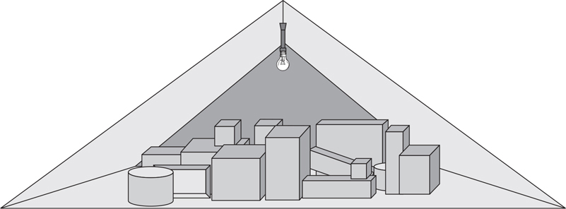
Figure 3-1 My attic, with no organization
Without some type of order placed on it, all the stuff in our home storage spaces becomes impossible to retrieve when we need it. The same is true in the world of electronic storage, as shown in Figure 3-2. Databases, like attics, need structure. Otherwise, we won’t be able to find anything!
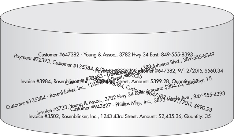
Figure 3-2 An unorganized database
The first step in getting organized is to have a place for everything and to have everything in its place. To achieve this, you need to add structure to the storage space, whether this is a space for box storage, like my attic, or a space for data storage, like a database. To maintain this structure, you also need to have discipline of one sort or another as you add items to the storage space.
To get my attic organized, I need some shelves, a few labels, and some free time so I can add the much-needed structure to this storage space. To keep my attic organized, I also need the discipline to pay attention to my new signs each time I put another box into storage. Figure 3-3 shows my attic as it exists in my fantasy world, where I have tons of free time and loads of self-discipline.
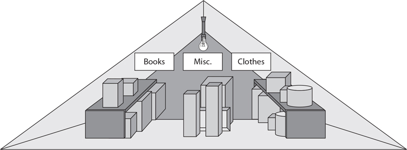
Figure 3-3 My attic in my fantasy world
Structure in the database world comes in the form of tables. Each database is divided into a number of tables. These tables store the information. Each table contains only one type of information. Figure 3-4 shows customer information in one table, payment information in another, and invoice header information in a third.
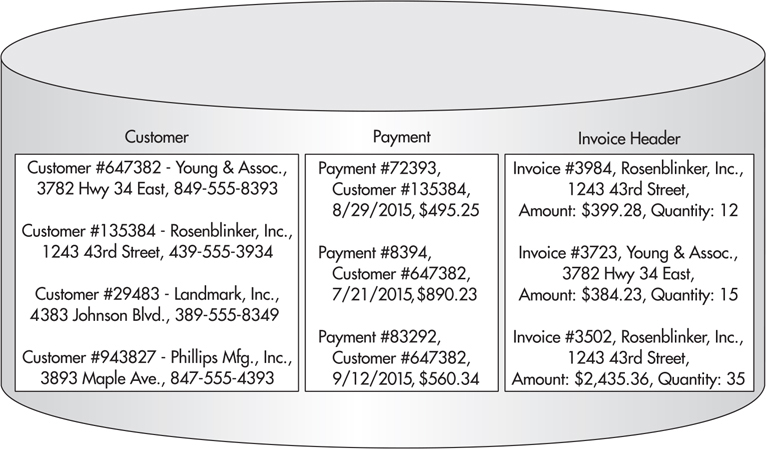
Figure 3-4 A database organized by tables
 NOTE
NOTE
Invoice Header is used as the name of the third table for consistency with the sample database that will be introduced in the section “Galactic Delivery Services” and used throughout the remainder of the book. The Invoice Header name helps to differentiate this table from the Invoice Detail table that stores the detail lines of the invoice. The Invoice Detail table is not discussed here, but it will be present in the sample database.
Dividing each table into rows and columns brings additional structure to the database. Figure 3-5 shows the Customer table divided into several rows—one row for each customer whose information is being stored in the table. In addition, the Customer table is divided into a number of columns. Each column is given a name: Customer Number, Customer Name, Address, and Phone. These names tell you what information is being stored in each column.
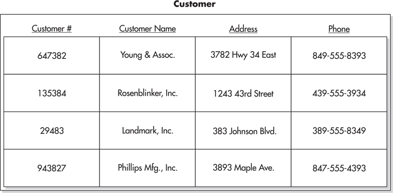
Figure 3-5 A database table organized by rows and columns
With a database structured as tables, rows, and columns, you know exactly where to find a certain piece of information. For example, it is pretty obvious that the customer name for customer number 135384 will be found in the Name column of the second row of the Customer table. We are starting to get this data organized, and it was a lot easier than cleaning out the attic!
Rows in a database are also called “records”. Columns in a database are also called “fields”. Reporting Services uses the terms “rows” and “records” interchangeably. It also uses the terms “columns” and “fields” interchangeably. Don’t be confused by this!
Columns also force some discipline on anyone putting data into the table. Each column has certain characteristics assigned to it. For instance, the Customer Number column in Figure 3-5 may only contain strings of digits (0–9); no letters (A–Z) are allowed. It is also limited to a maximum of six characters. In data design lingo, these are known as constraints. Given these constraints, it is impossible to store a customer’s name in the Customer Number column. The customer’s name is likely too long and contains characters that are not legal in the Customer Number column. Constraints provide the discipline to force organization within a database.
Typically, when you design a database, you create tables for each of the things you want to keep track of. In Figure 3-4, the database designer knew that her company needed to track information for customers, payments, and invoices. Database designers call these things entities. The database designer created tables for the customer, payment, and invoice header entities. These tables are named Customer, Payment, and Invoice Header.
Once the entities have been identified, the database designer determines what information needs to be known about each entity. In Figure 3-5, the designer identified the customer number, customer name, address, and phone number as the things that need to be known for each customer. These are attributes of the customer entity. The database designer creates a column in the Customer table for each of these attributes.
As entities and attributes are being defined, the database designer needs to identify a special attribute for each entity in the database. This special attribute is known as the primary key. The purpose of the primary key is to uniquely identify a single entity or, in the case of a database table, a single row in the table.
Two simple rules exist for primary keys. First, every entity must have a primary key value. Second, no two rows in an entity can have the same primary key value. In Figure 3-5, the Customer Number column can serve as the primary key. Every customer is assigned a customer number, and no two customers can be assigned the same customer number.
For most entities, the primary key is a single attribute. However, in some cases, two attributes must be combined to create a unique primary key. This is known as a composite primary key. For instance, if you were defining an entity based on presidents of the United States, the first name would not be a valid primary key. John Adams, John Quincy Adams, and John Kennedy all have the same first name. You would need to create a composite key combining first name, middle name, and last name to have a valid primary key.
As the database designer continues to work on identifying entities and attributes, she will notice that two different entities have some of the same attributes. For example, in Figure 3-6, both the customer entity and the invoice header entity have attributes of Customer Name and Address. This duplication of information seems rather wasteful. Not only are the customer’s name and address duplicated between the Customer and Invoice Header tables, but they are also duplicated in several rows in the Invoice Header table itself.
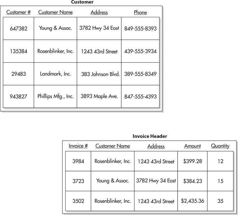
Figure 3-6 Database tables with duplicate data
The duplicate data also leads to another problem. Suppose that Rosenblinker, Inc., changes its name to RB, Inc. Then, Ann in the data-processing department changes the name in the Customer table because this is where we store information about the customer entity. However, the customer name has not been changed in the Invoice Header table. Because the customer name in the Invoice Header table no longer matches the customer name in the Customer table, it is no longer possible to determine how many invoices are outstanding for RB, Inc. Believe me, the accounting department will think this is a bad situation.
To avoid these types of problems, database tables are normalized. Normalization is a set of rules for defining database tables so each table contains attributes from only one entity. The rules for creating normalized database tables can be quite complex. You can hear database designers endlessly debating whether a proper database should be in 3rd normal form, 4th normal form, or 127th normal form. (Okay, there is no 127th normal form. I just made that up, but you get the point.) Let the database designers debate all they want. All you need to remember is this: a normalized database avoids data duplication.
A relation is a tool the database designer uses to avoid data duplication when creating a normalized database. A relation is simply a way to put the duplicated data in one place and then point to it from all the other places in the database where it would otherwise occur. The table that contains the data is called the parent table. The table that contains a pointer to the data in the parent table is called the child table. Just like parents and children of the human variety, the parent table and the child table are said to be related.
In our example, the customer name and address are stored in the Customer table. This is the parent table. A pointer is placed in the Invoice Header table in place of the duplicate customer names and addresses it had contained. The Invoice Header table is the child table.
As mentioned previously, each customer is uniquely identified by their customer number. Therefore, the Customer Number column serves as the primary key for the Customer table. In the Invoice Header table, we need a way to point to a particular customer. It makes sense to use the primary key from the parent table—in this case the Customer Number column—as that pointer. This is illustrated in Figure 3-7.
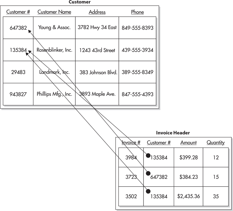
Figure 3-7 A database relation
Each row in the Invoice Header table now contains a copy of the primary key of a row in the Customer table. The Customer Number column in the Invoice Header table is called the foreign key. It is called a foreign key because it is not one of the native attributes of the invoice header entity. The customer number is a native attribute of the customer entity. The only reason the Customer Number column exists in the Invoice Header table is to create the relationship.
Let’s look back at the name change problem, this time using our new database structure that includes the parent-child relationship. When Rosenblinker, Inc., changes its name to RB, Inc., Ann changes the name in the Customer table as before. In our new structure, however, the customer name is not stored in any other location. Instead, the Invoice Header table rows for RB, Inc., point back to the Customer table row that has the correct name. The accounting department stays happy because it can still figure out how many invoices are outstanding for RB, Inc.
Database relations can be classified by the number of records that can exist on each side of the relationship. This is known as the cardinality of the relation. For example, the relation in Figure 3-7 is a one-to-many relation (in other words, one parent record can have many children). More specifically, one customer can have many invoices.
It is also possible to have a one-to-one relation. In this case, one parent record can have only one child. For example, let’s say our company rewards customers with a customer loyalty discount. Because only a few customers will receive this loyalty discount, we do not want to set aside space in every row in the Customer table to store the loyalty discount information. Instead, we create a new table to store this information. The new table is related to the Customer table, as shown in Figure 3-8. Our company’s business rule says that a given customer can only receive one loyalty discount. Because the Loyalty Discount table has only one Customer Number column, each row can link to just one customer. The combination of the business rule and the table design makes this a one-to-one relation.
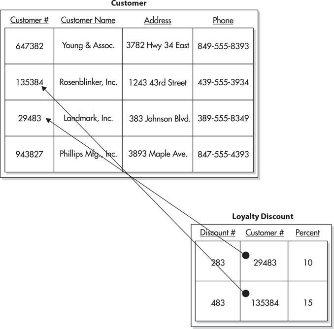
Figure 3-8 A one-to-one relation
It is also possible to have a many-to-many relation. This relation no longer fits our parent-child analogy. It is better thought of as a brother-sister relationship. One brother can have many sisters, and one sister can have many brothers.
Suppose we need to keep track of the type of business engaged in by each of our customers. We can add a Business Type table to our database, with columns for the business type code and the business type description. We can add a column for the business type code to the Customer table. We now have a one-to-many relation, where one business type can be related to many customers. This is shown in Figure 3-9.
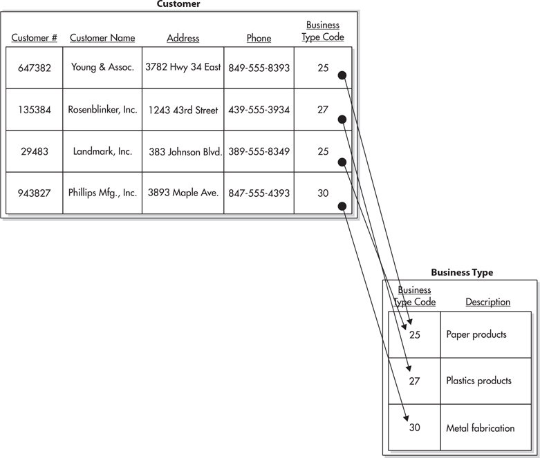
Figure 3-9 Tracking business type using a one-to-many relation
The problem with this structure becomes apparent when we have a customer that does multiple things. If Landmark, Inc., only produces paper products, there isn’t a problem. We can put the business type code for paper products in the Customer table row for Landmark, Inc. We run into a bit of a snag, however, if Landmark, Inc., also produces plastics. We could add a second business type code column to the Customer table, but this still limits a customer to a maximum of two business types. In today’s world of national conglomerates, this is not going to work.
The answer is to add a third table to the mix to create a many-to-many relation. This additional table is known as a linking table. Its only purpose is to link two other tables together in a many-to-many relation. To use a linking table, you create the Business Type table just as before. This time, however, instead of creating a new column in the Customer table, we’ll create a new table called Customer To Business Type Link. The new table has columns for the customer number and the business type code. Figure 3-10 shows how this linking table relates the Customer table to the Business Type table. By using the linking table, we can relate one customer to many business types. In addition, we can relate one business type to many customers.
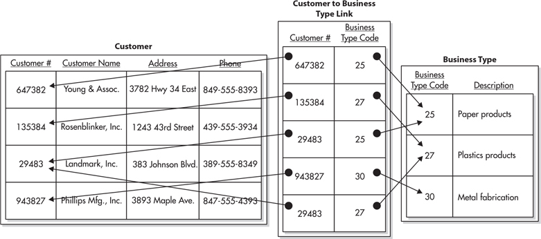
Figure 3-10 Tracking the business type using a many-to-many relation
We now have all the tools we need to store our data in an efficient manner. With our data structure set, it is time to determine how we can access that data to use it in our reports. Data that was split into multiple tables must be recombined for reporting. This is done using a database tool called a join. In most cases, we will also want the data in the report to appear in a certain order. This is accomplished using a sort.
Suppose we need to know the name and address of the customer associated with each invoice. This is certainly a reasonable request, especially if we want to send invoices to these clients and have those invoices paid. Checking the Invoice Header table, you can see it contains the customer number, but not the name and address. The name and address are stored in the Customer table.
To print our invoices, we need to join the data in the Customer table with the data in the Invoice Header table. This join is done by matching the customer number in each record of the Invoice Header table with the customer number in the Customer table. In the language of database designers, we are joining the Customer table to the Invoice Header table on the Customer Number column.
The result of the join is a new table that contains information from both the Customer table and the Invoice Header table in each row. This new table is known as a result set. The result set from the Customer table–to–Invoice Header table join is shown in Figure 3-11. Note that the result set table contains nearly the same information that was in the Invoice Header table before it was normalized. The result set is a denormalized form of the data in the database.
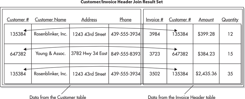
Figure 3-11 The result set from the Customer table–to–Invoice Header table join
It may seem like we are going in circles, first normalizing the data and then denormalizing it. There is, however, one important difference between the denormalized form of the Invoice Header table that we started with in Figure 3-6 and the result set in Figure 3-11. The denormalized result set is a temporary table: it exists only as long as it is needed; then it automatically goes away. The result set is re-created each time we execute the join, so the result set is always current.
Let’s return once more to Ann, our faithful employee in data processing. We will again consider the situation where Rosenblinker, Inc., changes its name to RB, Inc. Ann makes the change in the Customer table, as in the previous example. The next time we execute the join, this change is reflected in the result set. The result set has the new company name because our join gets a new copy of the customer information from the Customer table each time it is executed. The join finds the information in the Customer table based on the primary key, the customer number, which has not changed. Our invoices are linked to the proper companies, so accounting can determine how many invoices are outstanding for RB, Inc., and everyone is happy!
In the previous section, we looked at a type of join known as an inner join. When you do an inner join, your result set includes only those records that have a representative on both sides of the join. In Figure 3-11, Landmark, Inc., and Phillips Mfg., Inc., are not represented in the result set because they do not have any Invoice Header table rows linked to them.
Figure 3-12 shows another way to think about joins. Here, the two tables are shown as sets of customer numbers. The left-hand circle represents the set of customer numbers in the Customer table. It contains one occurrence of every customer number present in the Customer table. The right-hand circle represents the set of customer numbers in the Invoice Header table. It contains one occurrence of each customer number present in the Invoice Header table. The center region, where the two sets intersect, contains one occurrence of every customer number present in both the Customer table and the Invoice Header table. Looking at Figure 3-12, you can quickly tell that no customer numbers are present in the Invoice Header table that are not also present in the Customer table. This is as it should be. We should not have any invoice headers assigned to a customer that does not exist in the Customer table.
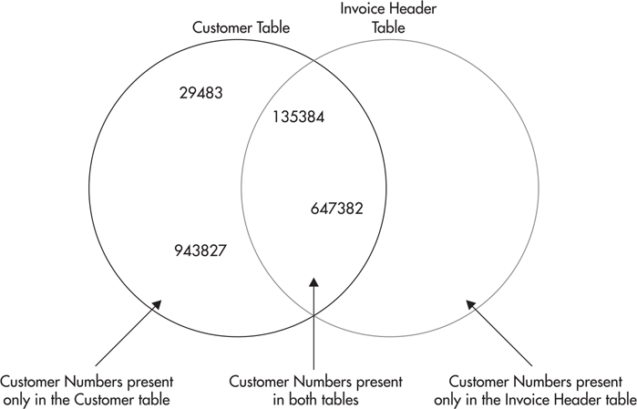
Figure 3-12 The set representation of the Customer and Invoice Header tables
Figure 3-13 shows a graphical representation of the inner join in Figure 3-11. Only records with customer numbers that appear in the shaded section will be included in the result set. Remember, two rows in the Invoice Header table contain customer number 135384. For this reason, the result set contains three rows—two rows for customer number 135384 and one row for customer number 647382.
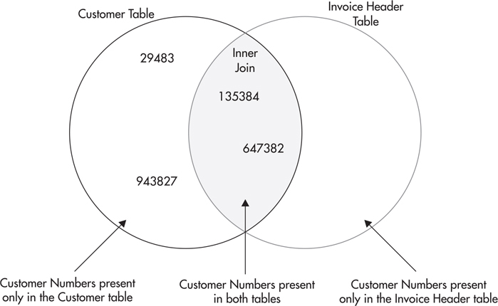
Figure 3-13 The set representation of the inner join of the Customer table and the Invoice Header table
The result set in Figure 3-11 enables us to print invoice headers that contain the correct customer name and address. Now let’s look at customers and invoice headers from a slightly different angle. Suppose we have been asked for a report showing all customers and the invoice headers that have been sent to them. If we were to print this customers/invoice headers report from the result set in Figure 3-11, it would exclude Landmark, Inc., and Phillips Mfg., Inc., because they do not have any invoices and, therefore, would not fulfill the requirements.
What we need is a result set that includes all the customers in the Customer table. This is illustrated graphically in Figure 3-14. This type of join is known as a left outer join so named because this join is not limited to the values in the intersection of both circles. It also includes the values to the left of the inner, overlapping sections of the circles.
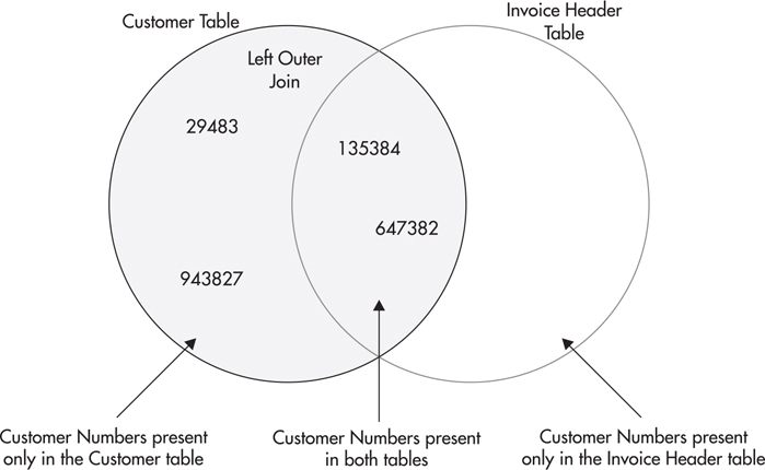
Figure 3-14 The set representation of the left outer join of the Customer table and the Invoice Header table
We can also perform a right outer join on two tables. In our example, a right outer join would return the same number of rows as the inner join. This is because no customer numbers are to the right of the intersection.
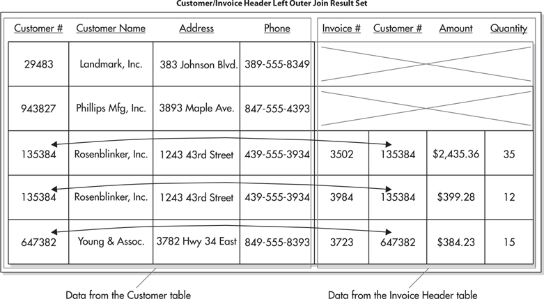
The result set produced by a left outer join of the Customer table and the Invoice Header table is shown in Figure 3-15. Notice the columns populated by data from the Invoice Header table are empty in rows for Landmark, Inc., and Phillips Mfg., Inc. The columns are empty because these two customers do not have any Invoice Header rows to provide data on the right side of the join.
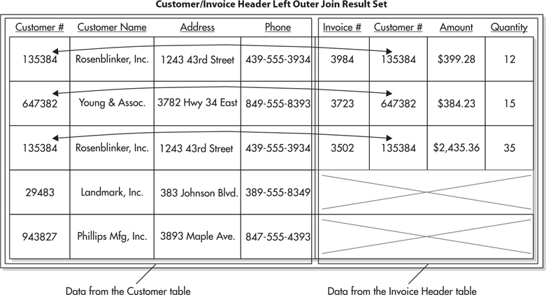
Figure 3-15 The result set from the left outer join of the Customer table and the Invoice Header table
Joins, whether inner or outer, always involve two tables. However, in Figure 3-10, you were introduced to a many-to-many relation that involved three tables. How do you retrieve data from this type of relation? The answer is to chain together two different joins, each involving two tables.
Figure 3-16 illustrates the joins required to reassemble the data from Figure 3-10. Here, the Customer table is joined to the Customer To Business Type Link table using the Customer Number column common to both tables. The Customer To Business Type Link table is then joined to the Business Type table using the Business Type Code column present in both tables. The final result set contains the data from all three tables.
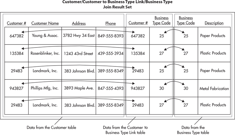
Figure 3-16 The result set from the join of the Customer table, the Customer To Business Type Link table, and the Business Type table
In our previous example, we needed to join three tables to get the required information. Other joins may only require a single table. For instance, we may have a customer that is a subsidiary of another one of our customers. In some cases, we’ll want to treat these two separately so both appear in our result set. This requires us to keep the two customers as separate rows in our Customer table. In other cases, we may want to combine information from the parent company and the subsidiary into one record. To do this, our database structure must include a mechanism to tie the subsidiary to its parent.
To track a customer’s connection to its parent, we need to create a relationship between the customer’s row in the Customer table and its parent’s row in the Customer table. To do this, we add a Parent Customer Number column to the Customer table, as shown in Figure 3-17. In the customer’s row, the Parent Customer Number column will contain the customer number of the row for the parent. In the row for the parent, and in all the rows for customers that do not have a parent, the Parent Customer Number column is empty.
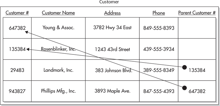
Figure 3-17 The customer/parent customer relation
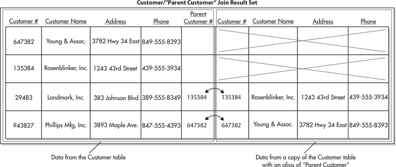
When we want to report from this parent/subsidiary relation, we need to do a join. This may seem like a problem at first because a join requires two tables and we only have one. The answer is to use the Customer table on one side of the join and a “copy” of the Customer table on the other side of the join. The second occurrence of the Customer table is given a nickname, called an alias so we can tell the two apart. This type of join, which uses the same table on both sides, is known as a self-join. Figure 3-18 shows the results of the self-join on the Customer table.
Figure 3-18 The result set from the Customer table self-join
In most cases, one final step is required before our result sets can be used for reporting. Let’s go back to the result set produced in Figure 3-15 for the customer/invoice header report. Looking back at this result set, notice the customers do not appear to be in any particular order. In most cases, users do not appreciate reports with information presented in this unsorted manner. This is especially true when two rows for the same customer do not appear consecutively, as is the case here.
We need to sort the result set as it is being created to avoid this situation. This is done by specifying the columns that should be used for the sort. Sorting by customer name probably makes the most sense for the customer/invoice header report. Columns can be sorted either in ascending order, smallest to largest (A–Z), or descending order, largest to smallest (Z–A). An ascending sort on Customer Name would be most appropriate.
We still have a situation where the order of the rows is left to chance. Because two rows have the same customer name, we do not know which of these two rows will appear first and which will appear second. A second sort field is necessary to break this “tie.” All the data copied into the result set from the Customer table will be the same in both of these rows. We need to look at the data copied from the Invoice Header table for a second sort column. In this case, an ascending sort on Invoice Number would be a good choice. Figure 3-19 shows the result set sorted by Customer Name, ascending, and then by Invoice Number, ascending.
Figure 3-19 The sorted result set from the left outer join of the Customer table and the Invoice Header table
Throughout the remainder of this book, you will get to know Reporting Services by exploring a number of sample reports. These reports will be based on the business needs of a company called Galactic Delivery Services (GDS). To better understand these sample reports, here is some background on GDS.

GDS provides package-delivery services between several planetary systems in the near galactic region. It specializes in rapid delivery featuring same-day, next-day, and previous-day delivery. The latter is made possible by its new Photon III transports, which travel faster than the speed of light. This faster-than-light capability allows GDS to exploit the properties of general relativity and deliver a package on the day before it was sent.
Despite GDS’s unique delivery offerings, it has the same data-processing needs as any more conventional package-delivery service. It tracks packages as they are moved from one interplanetary hub to another. This is important, not only for the smooth operation of the delivery service, but also to allow customers to check on the status of their delivery at any time.
To remain accountable to its clients and to prevent fraud, GDS investigates every package lost en route. These investigations help to find and eliminate problems throughout the entire delivery system. One such investigation discovered that a leaking antimatter valve on one of the Photon III transports was vaporizing two or three packages on each flight.
GDS stores its data in a database called Galactic. Figure 3-20 shows the portion of the Galactic database that stores the information used for package tracking. The tables and their column names are shown. A key symbol in the gray square next to a column name indicates this column is the primary key for that table. The lines connecting the tables show the relations that have been created between these tables in the database. The key symbol at the end of the line points to the primary key column used to create the relation. The infinity sign, at the opposite end of the line to the key symbol, points to the foreign key column used to complete the relation. (The infinity sign looks like two circles or a sideways number 8.)
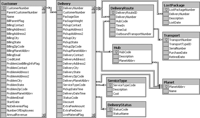
Figure 3-20 The package tracking tables from the Galactic database
Each relation shown in Figure 3-20 is a one-to-many relation. The side of the relation indicated by the key is the “one” side of the relation. The side indicated by the infinity sign is the “many” side of the relation. For example, if you look at the line between the Customer table and the Delivery table, you can see that one customer may have many deliveries.
You may want to refer to these diagrams as we create sample reports from the Galactic database. Don’t worry if the diagrams seem a bit complicated right now. They will make more sense as we consider the business practices and reporting needs at GDS. Also, our first report examples will contain only a few tables and the corresponding relations, so we will start simple and work our way up.
Every business needs a personnel department to look after its employees. GDS is no different. The GDS personnel department is responsible for the hiring and firing of all the robots employed by GDS. This department is also responsible for tracking the hours put in by the robotic laborers and paying them accordingly. (Yes, robots get paid at GDS. After all, GDS is an equal-opportunity employer.)
The personnel department is also responsible for conducting annual reviews of each employee. At the annual review, goals are set for the employee to attain over the coming year. After a year has passed, several of the employee’s co-workers are asked to rate the employee on how well it did in reaching those goals. The employee’s manager then uses the ratings to write an overall performance evaluation for the employee and establish new goals for the following year.
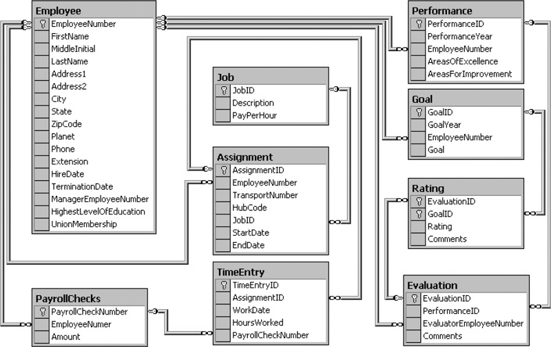
Figure 3-21 shows the tables in the Galactic database used by the personnel department. Notice that the Rating table has key symbols next to both the EvaluationID column name and the GoalID column name. This means the Rating table uses a composite primary key that combines the EvaluationID column and the GoalID column.
Figure 3-21 The personnel department tables from the Galactic database
The GDS accounting department is responsible for seeing that the company is paid for each package it delivers. GDS invoices its customers for each delivery completed. The invoices are sent to the customer, and payment is requested within 30 days.
Even though GDS delivers its customers’ packages at the speed of light, those same customers pay GDS at a much slower speed. “Molasses at the northern pole of Antares Prime” was the analogy used by the current chief financial droid. Therefore, GDS must track when invoices are paid, how much was paid, and how much is still outstanding.
Figure 3-22 shows the tables in the Galactic database used by the accounting department. Notice the Customer table appears in both Figure 3-20 and Figure 3-22. This is the same table in both diagrams. This table is shown in both because it is a major part of both the package tracking and the accounting business processes.
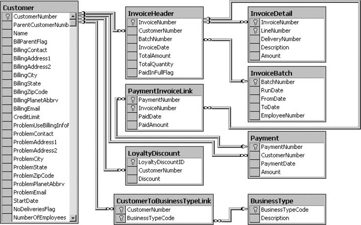
Figure 3-22 The accounting department tables from the Galactic database
In addition to all this, GDS must maintain a fleet of transports. Careful records are kept on the repair and preventative maintenance work done on each transport. GDS also has a record of each flight a transport makes, as well as any accidents and mishaps involved.
Maintenance records are extremely important, not only to GDS itself, but also to the Federation Space Flight Administration (FSFA). Without proper maintenance records on all its transports, GDS would be shut down by the FSFA in a nanosecond. You may think this is an exaggeration, but the bureaucratic androids at the FSFA have extremely high clock rates.
Figure 3-23 shows the transport maintenance tables in the Galactic database.
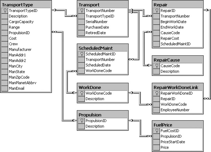
Figure 3-23 The transport maintenance tables from the Galactic database
You have now looked at the database concepts of normalization, relations, and joins. You have also been introduced to the Galactic database. We use this relational database throughout the remainder of this book for our examples. Now, it is time to look more specifically at how you retrieve the data from the database into a format you can use for reporting. This is done through the database query.
A query is a request for some action on the data in one or more tables. An INSERT query adds one or more rows to a database table. An UPDATE query modifies the data in one or more existing rows of a table. A DELETE query removes one or more rows from a table. Because we are primarily interested in retrieving data for reporting, the query we are going to concern ourselves with is the SELECT query which reads data from one or more tables (it does not add, update, or delete data).
We will look at the various parts of the SELECT query. This is to help you become familiar with this important aspect of reporting. The good news is Reporting Services provides a tool to guide you through the creation of queries, including the SELECT query. That tool is the Query Designer.
If you are familiar with SELECT queries and are more comfortable typing your queries from scratch, you can bypass the Query Designer and type in your queries directly. If SELECT queries are new to you, the following section can help you become familiar with the SELECT query and what it can do for you. Rest assured: the Query Designer enables you to take advantage of all the features of the SELECT query without having to memorize syntax or type a lot of code.
NOTE
If you have another query-creation tool you like to use instead of the Query Designer, you can create your queries with that tool and then copy them into the appropriate locations in the report definition.
The SELECT query is used to retrieve data from tables in the database. When a SELECT query is run, it returns a result set containing the selected data. With few exceptions, your reports will be built on result sets created by SELECT queries.
The SELECT query is often referred to as a SELECT statement. One reason for this is because it can be read like an English sentence or statement. As with a sentence in English, a SELECT statement is made up of clauses that modify the meaning of the statement.
The various parts, or clauses, of the SELECT statement enable you to control the data contained in the result set. Use the FROM clause to specify which table the data will be selected from. The FIELD LIST permits you to choose the columns that will appear in the result set. The JOIN clause lets you specify additional tables that will be joined with the table in the FROM clause to contribute data to the result set. The WHERE clause enables you to set conditions that determine which rows will be included in the result set. Finally, you can use the ORDER BY clause to sort the result set and the GROUP BY clause and the HAVING clause to combine detail rows into summary rows.
NOTE
The query statements shown in the remainder of this chapter all use the Galactic database. If you want to try out the various query statements as they are being discussed, open a query window for the Galactic database in SQL Server Management Studio. If you are not familiar with SQL Server Management Studio, you can try out the queries in the Reporting Services Generic Query Designer. To do this, turn to Chapter 5 and follow the steps for Task 1 of the Transport List Report. For SQL Server Data Tools and Visual Studio, stop after Step 29, and then click the Edit As Text button. For Report Builder, stop after Step 13, and then click the Edit As Text button. You will be in the Generic Query Designer. You can enter the query statements in the upper portion of the Generic Query Designer and execute them by clicking the toolbar button with the exclamation point (!). When you are finished, close the application without saving your changes.
The SELECT statement in its simplest form includes only a FROM clause. Here is a SELECT statement that retrieves all rows and all columns from the Customer table:
SELECT *FROM dbo.Customer
The word “SELECT” is required to let the database know this is going to be a SELECT query, as opposed to an INSERT, UPDATE, or DELETE query. The asterisk (*) means all columns will be included in the result set. The remainder of the statement is the FROM clause. It says the data is to be selected from the Customer table. We will discuss the meaning of “dbo.” in a moment.
As stated earlier, the SELECT statement can be read as if it were a sentence. This SELECT statement is read, “Select all columns from the Customer table.” If we run this SELECT statement in the Galactic database, the results would appear similar to Figure 3-24. The SELECT query is being run in the Query Designer window of SQL Server Data Tools. Note the scroll bars on the right and on the bottom of the result set area indicate that not all of the rows and columns returned can fit on the screen.
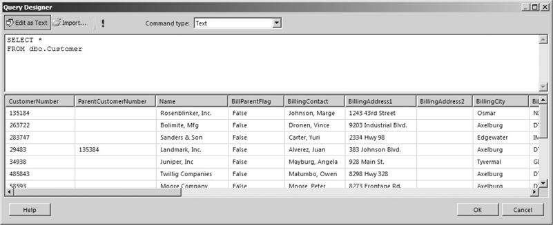
Figure 3-24 The SELECT statement in its simplest form
The table name, Customer, has “dbo.” in front of it. The dbo is the name of the schema the table is associated with. At its simplest, a schema is a way to group tables together inside a database. The default schema for tables in most cases is dbo. (The dbo stands for database owner, meaning the user who owns the database. This harkens back to a time in earlier versions of SQL Server where this prefix was tied to the user who created the table.)
In the Galactic database, the dbo.Customer table is part of the dbo schema. It would be possible for another Customer table, associated with a different schema, to be created in the Galactic database. For example, we could have an “xyz” schema and a table associated with that schema called xyz.Customer.
This situation, with two tables of the same name in the same database, does not happen often and is probably not a great idea. It can quickly lead to confusion and errors. Even though this is a rare occurrence, the Query Designer needs to account for this situation. The Query Designer uses both the name of the schema and the name of the table itself in the queries it builds and executes for you.
In the previous example, the result set created by the SELECT statement contained all of the columns in the table. In most cases, especially when creating reports, you only need to work with some of the columns of a table in any given result set. Including all of the columns in a result set when only a few columns are required wastes computing power and network bandwidth.
A FIELD LIST provides the capability you need to specify which columns to include in the result set. When a FIELD LIST is added to the SELECT statement, it appears similar to the following:
SELECT CustomerNumber, Name, BillingCityFROM dbo.Customer
The bold portion of the SELECT statement indicates changes from the previous SELECT statement.
This statement returns only the CustomerNumber, Name, and BillingCity columns from the Customer table. The result set created by this SELECT statement is shown in Figure 3-25.
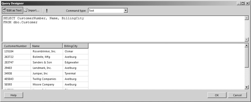
Figure 3-25 A SELECT statement with a FIELD LIST
NOTE
It is a good idea to get in the habit of always specifying a FIELD LIST in your queries rather than using the “*”. It will produce much more efficient queries, especially for tables that have a large number of columns.
In addition to the names of the fields to include in the result set, the FIELD LIST can contain a word that influences the number of rows in the result set. Usually, there is one row in the result set for each row in the table from which you are selecting data. However, this can be changed by adding the word “DISTINCT” at the beginning of the FIELD LIST.
When you use DISTINCT in the FIELD LIST, you are saying that you only want one row in the result set for each distinct set of values. In other words, the result set from a DISTINCT query will not include any two rows that have exactly the same values in every column. Here is an example of a DISTINCT query:
SELECT DISTINCT BillingCityFROM dbo.Customer
This query returns a list of all the billing cities in the Customer table. A number of customers have the same billing city, but these duplicates have been removed from the result set, as shown in Figure 3-26.
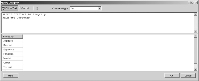
Figure 3-26 A DISTINCT query
When your database is properly normalized, you are likely to need data from more than one table to fulfill your reporting requirements. As discussed earlier in this chapter, the way to get information from more than one table is to use a join. The JOIN clause in the SELECT statement enables you to include a join of two or more tables in your result set.
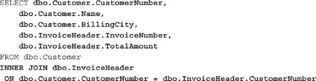
The first part of the JOIN clause specifies which table is being joined. The second part determines the two columns that are linked to create the join. Joining the Invoice Header table to the Customer table looks like this:
With the Customer table and the Invoice Header table joined, you have a situation where some columns in the result set have the same name. For example, a CustomerNumber column is present in the Customer table and a CustomerNumber column is present in the Invoice Header table. When you use the FIELD LIST to tell the database which fields to include in the result set, you need to uniquely identify these fields using both the table name and the column name.
If you do not do this, the query will not run and you will receive an error. Nothing prevents you from using the table name in front of each column name, whether it is a duplicate or not, as in this example. Using the table name in front of each column name makes it immediately obvious where every column in the result set is selected from. The result set created by this SELECT statement is shown in Figure 3-27.
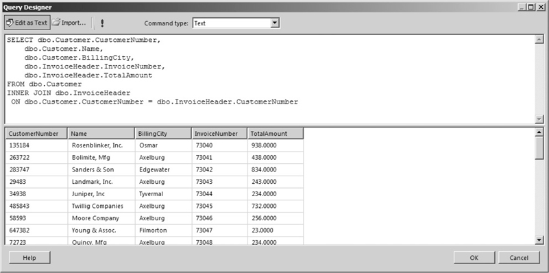
Figure 3-27 A SELECT statement with a JOIN clause
You can add a third table to the query by adding another JOIN clause to the SELECT statement. This additional table can be joined to the table in the FROM clause or to the table in the first JOIN clause. In this statement, we add the Loyalty Discount table and join it to the Customer table:
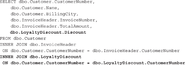
The result set from this SELECT statement is shown in Figure 3-28. Notice that the result set is rather small. This is because Landmark, Inc., is the only customer currently receiving a loyalty discount. Because an INNER JOIN was used to add the Loyalty Discount table, only customers that have a loyalty discount are included in the result set.
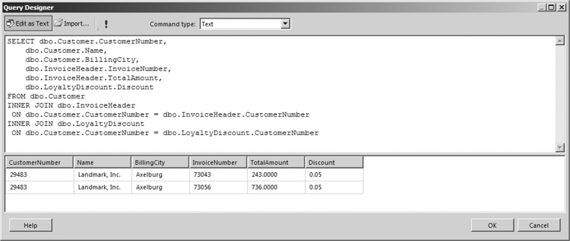
Figure 3-28 A SELECT statement with two JOIN clauses
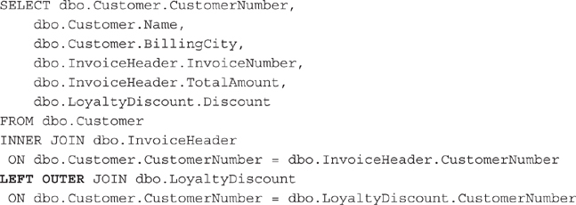
To make our result set a little more interesting, let’s try joining the Loyalty Discount table with an OUTER JOIN rather than an INNER JOIN. Here is the same statement, except the Customer table is joined to the Loyalty Discount table with a LEFT OUTER JOIN:
The result set for this SELECT statement is shown in Figure 3-29. Notice that the value for the Discount column is blank in the rows for all of the customers except for Landmark, Inc. (It is actually NULL, but this is being changed to a blank in the Query Designer display.) This blank value is to be expected, because there is no record in the Loyalty Discount table to join with these customers. When no value is in a column, the result set will contain a NULL value.
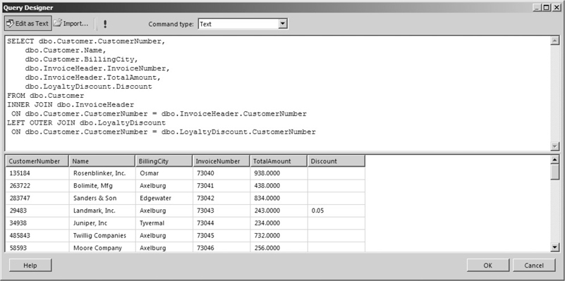
Figure 3-29 A SELECT statement with an INNER JOIN and an OUTER JOIN
Up to this point, the result sets have included all of the rows in the table or all of the rows that result from the joins. The FIELD LIST limits which columns are being returned in the result set. Nothing, however, placed a limit on the rows.
To limit the number of rows in the result set, you need to add a WHERE clause to your SELECT statement. The WHERE clause includes one or more logical expressions that must be true for a row before it can be included in the result set. Here is an example of a SELECT statement with a WHERE clause:
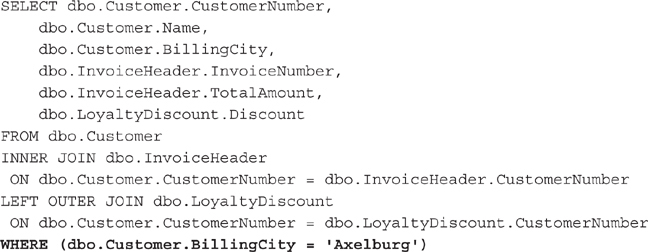
The word ‘Axelburg’ (enclosed in single quotes) is a string constant. A string constant also known as a string literal is an actual text value. The string constant instructs SQL Server to use the text between the single quotes as a value rather than the name of a column or a table. In this example, only customers with a value of Axelburg in their BillingCity column will be included in the result set, as shown in Figure 3-30.
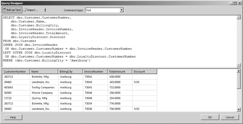
Figure 3-30 A SELECT statement with a WHERE clause
NOTE
Microsoft SQL Server 2016, in its standard configuration, insists on single quotes around string constants, such as ‘Axelburg’ in the previous SELECT statement. SQL Server 2016 assumes that anything enclosed in double quotes is a field name.
To create more complex criteria for your result set, you can have multiple logical expressions in the WHERE clause. The logical expressions are linked together with an AND or an OR. When an AND is used to link logical expressions, the logical expressions on both sides of the AND must be true for a row in order for that row to be included in the result set. When an OR is used to link two logical expressions, either one or both of the logical expressions must be true for a row in order for that row to be included in the result set.
This SELECT statement has two logical expressions in the WHERE clause:
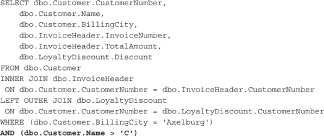
Only customers with a value of Axelburg in their BillingCity column and with a name that comes after C will be included in the result set. This result set is shown in Figure 3-31.
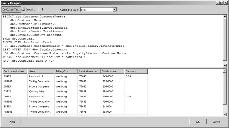
Figure 3-31 A SELECT statement with two logical expressions in the WHERE clause
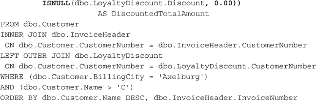
Up to this point, the data in the result sets has shown up in any order it pleases. As discussed previously, this will probably not be acceptable for most reports. You can add an ORDER BY clause to your SELECT statement to obtain a sorted result set. This statement includes an ORDER BY clause with multiple columns:
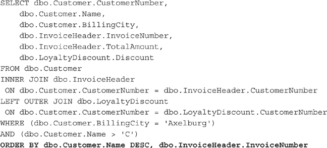
The result set created by this SELECT statement, shown in Figure 3-32, is first sorted by the contents of the Name column in the Customer table. The DESC that follows dbo.Customer.Name in the ORDER BY clause specifies the sort order for the customer name sort. DESC means this sort is done in descending order. In other words, the customer names will be sorted from the end of the alphabet to the beginning.
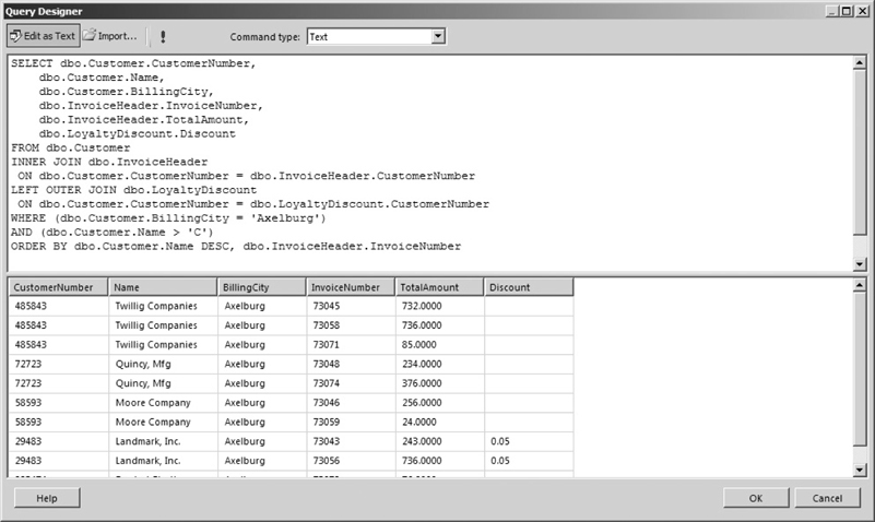
Figure 3-32 A SELECT statement with an ORDER BY clause
Several rows have the same customer name. For this reason, a second sort column is specified. This second sort is only applied within each group of identical customer names. For example, Twillig Companies has three rows in the result set. These three rows are sorted by the second sort, which is invoice number. No sort order is specified for the invoice number sort, so this defaults to an ascending sort. In other words, the invoice numbers are sorted from lowest to highest.
Our SELECT statement examples thus far have used an asterisk symbol or a FIELD LIST that includes only columns. A FIELD LIST can, in fact, include other things as well. For example, a FIELD LIST can include a constant value, as is shown here:
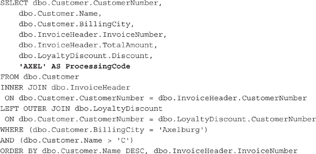
The string constant ‘AXEL’ has been added to the FIELD LIST. This creates a new column in the result set with the value AXEL in each row. By including AS ProcessingCode on this line, we give this result set column a name of ProcessingCode. Constant values of other data types, such as dates or numbers, can also be added to the FIELD LIST. The result set for this SELECT statement is shown in Figure 3-33.
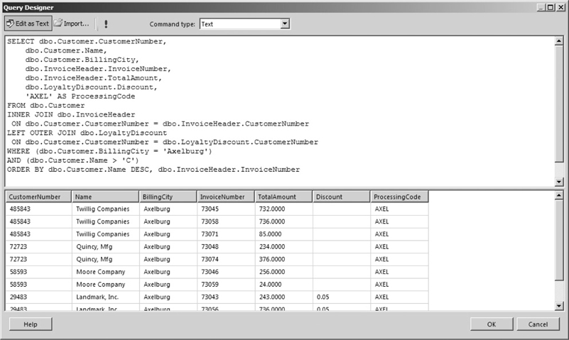
Figure 3-33 A SELECT statement with a constant in the FIELD LIST
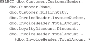
In addition to adding constant values, you can include calculations in the FIELD LIST. This SELECT statement calculates the discounted invoice amount based on the total amount of the invoice and the loyalty discount:
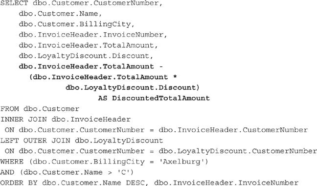
The result set for this SELECT statement is shown in Figure 3-34. Notice the value for the calculated column, DiscountedTotalAmount, is blank (actually NULL) for all the rows that are not for Landmark, Inc. This is because we are using the value of the Discount column in our calculation. The Discount column has a value of NULL for every row except for the Landmark, Inc., rows.
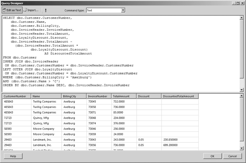
Figure 3-34 A SELECT statement with a calculated column in the FIELD LIST
A NULL value cannot be used successfully in any calculation. Any time you try to add, subtract, multiply, or divide a number by NULL, the result is NULL. The only way to receive a value in these situations is to give the database a valid value to use in place of any NULLs it might encounter. This is done using the ISNULL( ) function, as shown in the following statement:
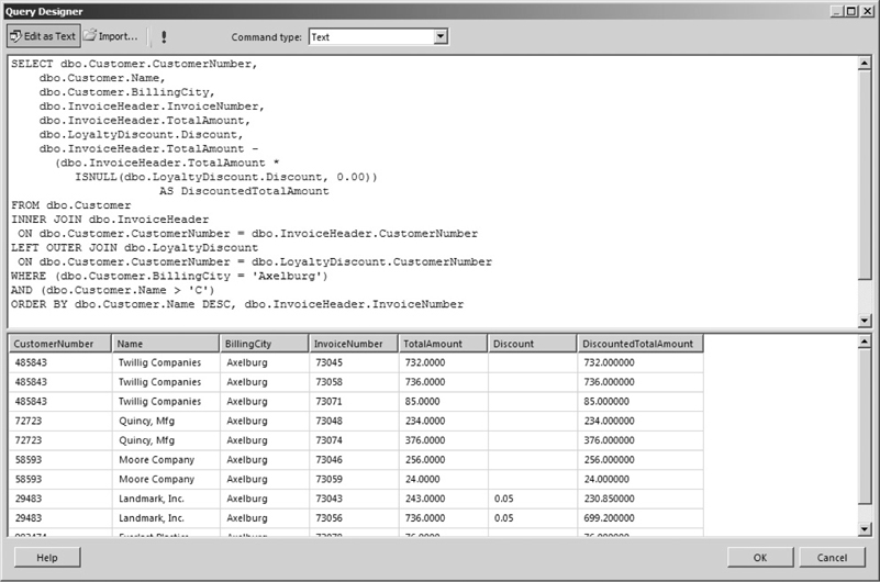
Now, when the database encounters a NULL value in the Discount column while it is performing the calculation, it substitutes a value of 0.00 and continues with the calculation. The database only performs this substitution when it encounters a NULL value. If any other value is in the Discount column, it uses that value. The result set from this SELECT statement is shown in Figure 3-35.
Figure 3-35 A SELECT statement using the ISNULL() function
Our sample SELECT statement appears to resemble a run-on sentence. You have seen, however, that each of these clauses is necessary to change the meaning of the statement and to provide the desired result set. We will add just two more clauses to the sample SELECT statement before we are done.
At times, as you are analyzing data, you only want to see information at a summary level, rather than viewing all the detail. In other words, you want the result set to group together the information from several rows to form a summary row. Additional instructions must be added to our SELECT statement in two places for this to happen.
First, you need to specify which columns are going to be used to determine when a summary row will be created. These columns are placed in the GROUP BY clause. Consider the following SELECT statement:
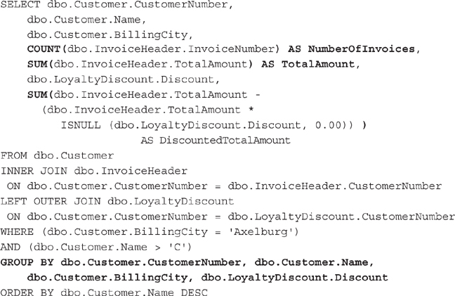
The CustomerNumber, Name, BillingCity, and Discount columns are included in the GROUP BY clause. When this query is run, each unique set of values from these four columns will result in a row in the result set.
Second, you need to specify how the columns in the FIELD LIST that are not included in the GROUP BY clause are to be handled. In the sample SELECT statement, the InvoiceNumber and TotalAmount columns are in the FIELD LIST, but are not part of the GROUP BY clause. The calculated column, DiscountedTotalAmount, is also in the FIELD LIST, but it is not present in the GROUP BY clause. In the sample SELECT statement, these three columns are the non–group-by columns.
The SELECT statement is asking for the values from several rows to be combined into one summary row. The SELECT statement needs to provide a way for this combining to take place. This is done by enclosing each non–group-by column in a special function called an aggregate function which performs a mathematical operation on values from a number of rows and returns a single result. The most commonly used aggregate functions include
SUM( ) Returns the sum of the values
AVG( ) Returns the average of the values
COUNT( ) Returns a count of the values
MAX( ) Returns the largest value
MIN( ) Returns the smallest value
The SELECT statement in our GROUP BY example uses the SUM( ) aggregate function to return the sum of the invoice amount and the sum of the discounted amount for each customer. It also uses the COUNT( ) aggregate function to return the number of invoices for each customer. The result set from this SELECT statement is shown in Figure 3-36. Note when an aggregate function is placed around a column name in the FIELD LIST, the SELECT statement can no longer determine what name to use for that column in the result set. You need to supply a column name to use in the result set, as shown in this SELECT statement.
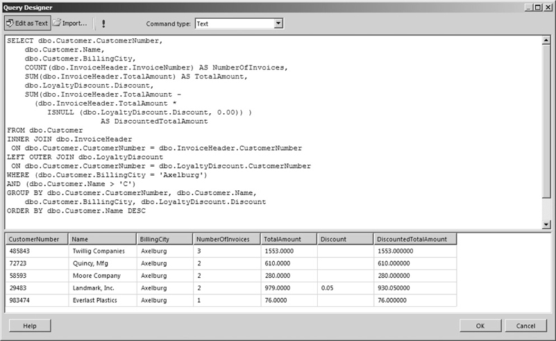
Figure 3-36 A SELECT statement with a GROUP BY clause
NOTE
When you’re using a GROUP BY clause, all columns in the FIELD LIST must either be included in the GROUP BY clause or be enclosed in an aggregate function. In the sample SELECT statement, the CustomerNumber column is all that is necessary in the GROUP BY clause to provide the desired grouping. However, because the Name, BillingCity, and Discount columns do not lend themselves to being aggregated, they are included in the GROUP BY clause along with the CustomerNumber column.
The GROUP BY clause has a special clause that can be used with it to determine which grouped rows will be included in the result set. This is the HAVING clause. The HAVING clause functions similarly to the WHERE clause. The WHERE clause limits the rows in the result set by checking conditions at the row level. The HAVING clause limits the rows in the result set by checking conditions at the group level.
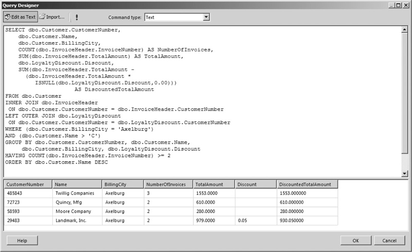
Consider the following SELECT statement:
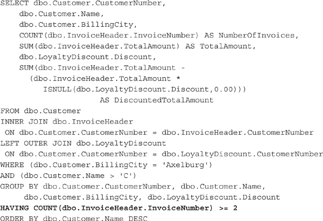
The WHERE clause says that a row must have a BillingCity column with a value of Axelburg and a Name column with a value greater than C before it can be included in the group. The HAVING clause says a group must contain at least two invoices before it can be included in the result set. The result set for this SELECT statement is shown in Figure 3-37.
Figure 3-37 A SELECT statement with a HAVING clause
Good reporting depends more on getting the right data out of the database than it does on creating a clean report design and delivering the report in a timely manner. If you are feeling a little overwhelmed by the workings of relational databases and SELECT queries, don’t worry. Refer to this chapter from time to time if you need to.
Also, remember Reporting Services provides you with the Query Designer tool to assist with the query-creation process. You needn’t remember the exact syntax for the LEFT OUTER JOIN or a GROUP BY clause. What you do need to know are the capabilities of the SELECT statement so you know what to instruct the Query Designer to create.
Finally, when you are creating your queries, use the same method that was used here: in other words, build them one step at a time. Join together the tables you will need for your report, determine what columns are required, and then come up with a WHERE clause that gets you only the rows you are looking for. After that, you can add in the sorting and grouping. Assemble one clause, and then another and another, and pretty soon, you will have a slam-bang query that will give you exactly the data you need!
Now, on to the reports….