we obtain the result

E[T]=3λ1+λ2

Another way to obtain E[T] is to write T as a sum, take expectations, and then condition where needed. This approach yields

E[T]=E[min(R1,R2)+S]=E[min(R1,R2)]+E[S]=1λ1+λ2+E[S]

To compute E[S], we condition on which of R1 and R2 is smallest.

E[S]=E[S∣R1<R2]λ1λ1+λ2+E[S∣R2⩽R1]λ2λ1+λ2=2λ1+λ2■

Example 5.9

There are n cells in the body, of which cells 1,…,k are target cells. Associated with each cell is a weight, with wi being the weight associated with cell i,i=1,…,n. The cells are destroyed one at a time in a random order, which is such that if S is the current set of surviving cells then, independent of the order in which the cells not in S have been destroyed, the next cell killed is i,i∈S, with probability wi/∑j∈Swj. In other words, the probability that a given surviving cell is the next one to be killed is the weight of that cell divided by the sum of the weights of all still surviving cells. Let A denote the total number of cells that are still alive at the moment when all the cells 1,2,…,k have been killed, and find E[A].

Solution: Although it would be quite difficult to solve this problem by a direct combinatorial argument, a nice solution can be obtained by relating the order in which cells are killed to a ranking of independent exponential random variables. To do so, let X1,…,Xn be independent exponential random variables, with Xi having rate wi,i=1,…,n. Note that Xi will be the smallest of these exponentials with probability wi/∑jwj; further, given that Xi is the smallest, Xr will be the next smallest with probability wr/∑j≠iwj; further, given that Xi and Xr are, respectively, the first and second smallest, Xs, s≠i,r, will be the third smallest with probability ws/∑j≠i,rwj; and so on. Consequently, if we let Ij be the index of the jth smallest of X1,…,Xn—so that XI1<XI2<⋯<XIn—then the order in which the cells are destroyed has the same distribution as I1,…,In. So, let us suppose that the order in which the cells are killed is determined by the ordering of X1,…,Xn. (Equivalently, we can suppose that all cells will eventually be killed, with cell i being killed at time Xi,i=1,…,n.)
If we let Aj equal 1 if cell j is still alive at the moment when all the cells 1,…,k have been killed, and let it equal 0 otherwise, then

A=∑j=k+1nAj

Because cell j will be alive at the moment when all the cells 1,…,k have been killed if Xj is larger than all the values X1,…,Xk, we see that for j>k

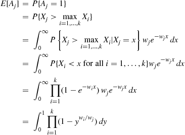
E[Aj]=P{Aj=1}=P{Xj>maxi=1,…,kXi}=∫0∞PXj>maxi=1,…,kXi∣Xj=xwje-wjxdx=∫0∞P{Xi<xfor alli=1,…,k}wje-wjxdx=∫0∞∏i=1k(1-e-wix)wje-wjxdx=∫01∏i=1k(1-ywi/wj)dy

where the final equality follows from the substitution y=e-wjx. Thus, we obtain the result

E[A]=∑j=k+1n∫01∏i=1k(1-ywi/wj)dy=∫01∑j=k+1n∏i=1k(1-ywi/wj)dy■

Example 5.10

Suppose that customers are in line to receive service that is provided sequentially by a server; whenever a service is completed, the next person in line enters the service facility. However, each waiting customer will only wait an exponentially distributed time with rate θ; if its service has not yet begun by this time then it will immediately depart the system. These exponential times, one for each waiting customer, are independent. In addition, the service times are independent exponential random variables with rate μ. Suppose that someone is presently being served and consider the person who is nth in line.

(a) Find Pn, the probability that this customer is eventually served.

(b) Find Wn, the conditional expected amount of time this person spends waiting in line given that she is eventually served.

Solution: Consider the n+1 random variables consisting of the remaining service time of the person in service along with the n additional exponential departure times with rate θ of the first n in line.
(a) Given that the smallest of these n+1 independent exponentials is the departure time of the nth person in line, the conditional probability that this person will be served is 0; on the other hand, given that this person’s departure time is not the smallest, the conditional probability that this person will be served is the same as if it were initially in position n-1. Since the probability that a given departure time is the smallest of the n+1 exponentials is θ/(nθ+μ), we obtain

Pn=(n-1)θ+μnθ+μPn-1

Using the preceding with n-1 replacing n gives

Pn=(n-1)θ+μnθ+μ(n-2)θ+μ(n-1)θ+μPn-2=(n-2)θ+μnθ+μPn-2

Continuing in this fashion yields the result

Pn=θ+μnθ+μP1=μnθ+μ

(b) To determine an expression for Wn, we use the fact that the minimum of independent exponentials is, independent of their rank ordering, exponential with a rate equal to the sum of the rates. Since the time until the nth person in line enters service is the minimum of these n+1 random variables plus the additional time thereafter, we see, upon using the lack of memory property of exponential random variables, that

Wn=1nθ+μ+Wn-1

Repeating the preceding argument with successively smaller values of n yields the solution

Wn=∑i=1n1iθ+μ■

5.2.4 Convolutions of Exponential Random Variables

Let Xi,i=1,…,n, be independent exponential random variables with respective rates λi,i=1,…,n, and suppose that λi≠λj for i≠j. The random variable ∑i=1nXi is said to be a hypoexponential random variable. To compute its probability density function, let us start with the case n=2. Now,

fX1+X2(t)=∫0tfX1(s)fX2(t-s)ds=∫0tλ1e-λ1sλ2e-λ2(t-s)ds=λ1λ2e-λ2t∫0te-(λ1-λ2)sds=λ1λ1-λ2λ2e-λ2t(1-e-(λ1-λ2)t)=λ1λ1-λ2λ2e-λ2t+λ2λ2-λ1λ1e-λ1t

Using the preceding, a similar computation yields, when n=3,

fX1+X2+X3(t)=∑i=13λie-λit∏j≠iλjλj-λi

which suggests the general result

fX1+⋯+Xn(t)=∑i=1nCi,nλie-λit

where

Ci,n=∏j≠iλjλj-λi

We will now prove the preceding formula by induction on n. Since we have already established it for n=2, assume it for n and consider n+1 arbitrary independent exponentials Xi with distinct rates λi,i=1,…,n+1. If necessary, renumber X1 and Xn+1 so that λn+1<λ1. Now,

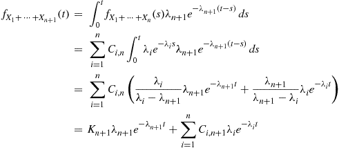
fX1+⋯+Xn+1(t)=∫0tfX1+⋯+Xn(s)λn+1e-λn+1(t-s)ds=∑i=1nCi,n∫0tλie-λisλn+1e-λn+1(t-s)ds=∑i=1nCi,nλiλi-λn+1λn+1e-λn+1t+λn+1λn+1-λiλie-λit=Kn+1λn+1e-λn+1t+∑i=1nCi,n+1λie-λit (5.7)

(5.7)

where Kn+1=∑i=1nCi,nλi/(λi-λn+1) is a constant that does not depend on t. But, we also have that

fX1+⋯+Xn+1(t)=∫0tfX2+⋯+Xn+1(s)λ1e-λ1(t-s)ds

which implies, by the same argument that resulted in Equation (5.7), that for a constant K1

fX1+⋯+Xn+1(t)=K1λ1e-λ1t+∑i=2n+1Ci,n+1λie-λit

Equating these two expressions for fX1+⋯+Xn+1(t) yields

Kn+1λn+1e-λn+1t+C1,n+1λ1e-λ1t=K1λ1e-λ1t+Cn+1,n+1λn+1e-λn+1t

Multiplying both sides of the preceding equation by eλn+1t and then letting t→∞ yields [since e-(λ1-λn+1)t→0 as t→∞]

Kn+1=Cn+1,n+1

and this, using Equation (5.7), completes the induction proof. Thus, we have shown that if S=∑i=1nXi, then

fS(t)=∑i=1nCi,nλie-λit (5.8)

(5.8)

where

Ci,n=∏j≠iλjλj-λi

Integrating both sides of the expression for fS from t to ∞ yields that the tail distribution function of S is given by

P{S>t}=∑i=1nCi,ne-λit (5.9)

(5.9)

Hence, we obtain from Equations (5.8) and (5.9) that rS(t), the failure rate function of S, is as follows:

rS(t)=∑i=1nCi,nλie-λit∑i=1nCi,ne-λit

If we let λj=min(λ1,…,λn), then it follows, upon multiplying the numerator and denominator of rS(t) by eλjt, that

limt→∞rS(t)=λj

From the preceding, we can conclude that the remaining lifetime of a hypoexponentially distributed item that has survived to age t is, for t large, approximately that of an exponentially distributed random variable with a rate equal to the minimum of the rates of the random variables whose sums make up the hypoexponential.

Remark

Although

1=∫0∞fS(t)dt=∑i=1nCi,n=∑i=1n∏j≠iλjλj-λi

it should not be thought that the Ci,n,i=1,…,n are probabilities, because some of them will be negative. Thus, while the form of the hypoexponential density is similar to that of the hyperexponential density (see Example 5.6) these two random variables are very different.

Example 5.11

Let X1,…,Xm be independent exponential random variables with respective rates λ1,…,λm, where λi≠λj when i≠j. Let N be independent of these random variables and suppose that ∑n=1mPn=1, where Pn=P{N=n}. The random variable

Y=∑j=1NXj

is said to be a Coxian random variable. Conditioning on N gives its density function:

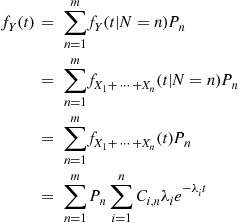
fY(t)=∑n=1mfY(t∣N=n)Pn=∑n=1mfX1+⋯+Xn(t∣N=n)Pn=∑n=1mfX1+⋯+Xn(t)Pn=∑n=1mPn∑i=1nCi,nλie-λit

Let

r(n)=P{N=n∣N⩾n}

If we interpret N as a lifetime measured in discrete time periods, then r(n) denotes the probability that an item will die in its nth period of use given that it has survived up to that time. Thus, r(n) is the discrete time analog of the failure rate function r(t), and is correspondingly referred to as the discrete time failure (or hazard) rate function.

Coxian random variables often arise in the following manner. Suppose that an item must go through m stages of treatment to be cured. However, suppose that after each stage there is a probability that the item will quit the program. If we suppose that the amounts of time that it takes the item to pass through the successive stages are independent exponential random variables, and that the probability that an item that has just completed stage n quits the program is (independent of how long it took to go through the n stages) equal to r(n), then the total time that an item spends in the program is a Coxian random variable. ■

5.3 The Poisson Process

5.3.1 Counting Processes

A stochastic process {N(t),t⩾0} is said to be a counting process if N(t) represents the total number of “events” that occur by time t. Some examples of counting processes are the following:

(a) If we let N(t) equal the number of persons who enter a particular store at or prior to time t, then {N(t),t⩾0} is a counting process in which an event corresponds to a person entering the store. Note that if we had let N(t) equal the number of persons in the store at time t, then {N(t),t⩾0} would not be a counting process (why not?).

(b) If we say that an event occurs whenever a child is born, then {N(t),t⩾0} is a counting process when N(t) equals the total number of people who were born by time t. (Does N(t) include persons who have died by time t? Explain why it must.)

(c) If N(t) equals the number of goals that a given soccer player scores by time t, then {N(t),t⩾0} is a counting process. An event of this process will occur whenever the soccer player scores a goal.

From its definition we see that for a counting process N(t) must satisfy:

(i) N(t)⩾0.

(ii) N(t) is integer valued.

(iii) If s<t, then N(s)⩽N(t).

(iv) For s<t,N(t)-N(s) equals the number of events that occur in the interval (s,t].

A counting process is said to possess independent increments if the numbers of events that occur in disjoint time intervals are independent. For example, this means that the number of events that occur by time 10 (that is, N(10)) must be independent of the number of events that occur between times 10 and 15 (that is, N(15)-N(10)).

The assumption of independent increments might be reasonable for example (a), but it probably would be unreasonable for example (b). The reason for this is that if in example (b) N(t) is very large, then it is probable that there are many people alive at time t; this would lead us to believe that the number of new births between time t and time t+s would also tend to be large (that is, it does not seem reasonable that N(t) is independent of N(t+s)-N(t), and so {N(t),t⩾0} would not have independent increments in example (b)). The assumption of independent increments in example (c) would be justified if we believed that the soccer player’s chances of scoring a goal today do not depend on “how he’s been going.” It would not be justified if we believed in “hot streaks” or “slumps.”

A counting process is said to possess stationary increments if the distribution of the number of events that occur in any interval of time depends only on the length of the time interval. In other words, the process has stationary increments if the number of events in the interval (s,s+t) has the same distribution for all s.

The assumption of stationary increments would only be reasonable in example (a) if there were no times of day at which people were more likely to enter the store. Thus, for instance, if there was a rush hour (say, between 12 P.M. and 1 P.M.) each day, then the stationarity assumption would not be justified. If we believed that the earth’s population is basically constant (a belief not held at present by most scientists), then the assumption of stationary increments might be reasonable in example (b). Stationary increments do not seem to be a reasonable assumption in example (c) since, for one thing, most people would agree that the soccer player would probably score more goals while in the age bracket 25–30 than he would while in the age bracket 35–40. It may, however, be reasonable over a smaller time horizon, such as one year.

5.3.2 Definition of the Poisson Process

One of the most important types of counting process is the Poisson process. As a prelude to giving its definition, we define the concept of a function f(·) being o(h).

Definition 5.1

The function f(·) is said to be o(h) if

limh→0f(h)h=0

Example 5.12

(a) The function f(x)=x2 is o(h) since

limh→0f(h)h=limh→0h2h=limh→0h=0

(b) The function f(x)=x is not o(h) since

limh→0f(h)h=limh→0hh=limh→01=1≠0

(c) If f(·) is o(h) and g(·) is o(h), then so is f(·)+g(·). This follows since

limh→0f(h)+g(h)h=limh→0f(h)h+limh→0g(h)h=0+0=0

(d) If f(·) is o(h), then so is g(·)=cf(·). This follows since

limh→0cf(h)h=climf(h)h=c·0=0

(e) From (c) and (d) it follows that any finite linear combination of functions, each of which is o(h), is o(h). ■

In order for the function f(·) to be o(h) it is necessary that f(h)/h go to zero as h goes to zero. But if h goes to zero, the only way for f(h)/h to go to zero is for f(h) to go to zero faster than h does. That is, for h small, f(h) must be small compared with h.

The o(h) notation can be used to make statements more precise. For instance, if X is continuous with density f and failure rate function λ(t), then the approximate statements

P(t<X<t+h)≈f(t)hP(t<X<t+h∣X>t)≈λ(t)h

can be precisely expressed as

P(t<X<t+h)=f(t)h+o(h)P(t<X<t+h∣X>t)=λ(t)h+o(h)

We are now in position to define the Poisson process.

Definition 5.2

The counting process {N(t),t⩾0} is said to be a Poisson process with rate λ>0 if the following axioms hold:

(i) N(0)=0

(ii) {N(t),t⩾0}has independent increments

(iii) P(N(t+h)-N(t)=1)=λh+o(h)

(iv) P(N(t+h)-N(t)⩾2)=o(h)

The preceding is called a Poisson process because the number of events in any interval of length t is Poisson distributed with mean λt, as is shown by the following important theorem.

Theorem 5.1

If {N(t),t⩾0} is a Poisson process with rate λ>0, then for all s>0,t>0, N(s+t)-N(s) is a Poisson random variable with mean λt. That is, the number of events in any interval of length t is a Poisson random variable with mean λt.

Proof

We begin by deriving E[e-uN(t)], the Laplace transform of N(t). To do so, fix u>0 and define

g(t)=E[e-uN(t)]

We will obtain g(t) by deriving a differential equation as follows.

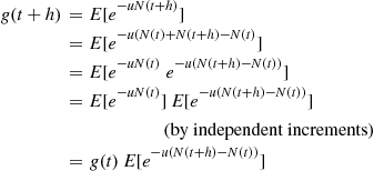
g(t+h)=E[e-uN(t+h)]=E[e-u(N(t)+N(t+h)-N(t)]=E[e-uN(t)e-u(N(t+h)-N(t))]=E[e-uN(t)]E[e-u(N(t+h)-N(t))](by independent increments)=g(t)E[e-u(N(t+h)-N(t))] (5.10)

(5.10)

Now, from Axioms (iii) and (iv)

P{N(t+h)-N(t)=0}=1-λh+o(h)P{N(t+h)-N(t)=1}=λh+o(h)P{N(t+h)-N(t)⩾2}=o(h)

Conditioning on which of these three possibilities occurs gives that

E[e-u[N(t+h)-N(t)]]=1-λh+o(h)+e-u(λh+o(h))+o(h)=1-λh+e-uλh+o(h) (5.11)

(5.11)

Therefore, from Equations (5.10) and (5.11) we obtain

g(t+h)=g(t)(1+λh(e-u-1)+o(h))

which can be written as

g(t+h)-g(t)h=g(t)λ(e-u-1)+o(h)h

Letting h→0 yields the differential equation

g′(t)=g(t)λ(e-u-1)

or

g′(t)g(t)=λ(e-u-1)

Noting that the left side is the derivative of log(g(t)) yields, upon integration, that

log(g(t))=λ(e-u-1)t+C

Because g(0)=E[e-uN(0)]=1 it follows that C=0, and so the Laplace transform of N(t) is

E[e-uN(t)]=g(t)=eλt(e-u-1)

However, if X is a Poisson random variable with mean λt, then its Laplace transform is

E[e-uX]=∑ie-uie-λt(λt)i/i!=e-λt∑i(λte-u)i/i!=e-λteλte-u=eλt(e-u-1)

Because the Laplace transform uniquely determines the distribution, we can thus conclude that N(t) is Poisson with mean λt.

To show that N(s+t)-N(s) is also Poisson with mean λt, fix s and let Ns(t)=N(s+t)-N(s) equal the number of events in the first t time units when we start our count at time s. It is now straightforward to verify that the counting process {Ns(t),t⩾0} satisfies all the axioms for being a Poisson process with rate λ. Consequently, by our preceding result, we can conclude that Ns(t) is Poisson distributed with mean λt. ■

Remarks

(i) The result that N(t), or more generally N(t+s)-N(s), has a Poisson distribution is a consequence of the Poisson approximation to the binomial distribution (see Section 2.2.4). To see this, subdivide the interval [0,t] into k equal parts where k is very large (Figure 5.1). Now it can be shown using axiom (iv) of Definition 5.2 that as k increases to ∞ the probability of having two or more events in any of the k subintervals goes to 0. Hence, N(t) will (with a probability going to 1) just equal the number of subintervals in which an event occurs. However, by stationary and independent increments this number will have a binomial distribution with parameters k and p=λt/k+o(t/k). Hence, by the Poisson approximation to the binomial we see by letting k approach ∞ that N(t) will have a Poisson distribution with mean equal to

limk→∞kλtk+otk=λt+limk→∞to(t/k)t/k=λt

by using the definition of o(h) and the fact that t/k→0 as k→∞.

(ii) Because the distribution of N(t+s)-N(s) is the same for all s, it follows that the Poisson process has stationary increments.

Figure 5.1

5.3.3 Interarrival and Waiting Time Distributions

Consider a Poisson process, and let us denote the time of the first event by T1. Further, for n>1, let Tn denote the elapsed time between the (n-1)st and the nth event. The sequence {Tn,n=1,2,…} is called the sequence of interarrival times. For instance, if T1=5 and T2=10, then the first event of the Poisson process would have occurred at time 5 and the second at time 15.

We shall now determine the distribution of the Tn. To do so, we first note that the event {T1>t} takes place if and only if no events of the Poisson process occur in the interval [0,t] and thus,

P{T1>t}=P{N(t)=0}=e-λt

Hence, T1 has an exponential distribution with mean 1/λ. Now,

P{T2>t}=E[P{T2>t∣T1}]

However,

P{T2>t∣T1=s}=P{0eventsin(s,s+t]∣T1=s}=P{0eventsin(s,s+t]}=e-λt (5.12)

(5.12)

where the last two equations followed from independent and stationary increments. Therefore, from Equation (5.12) we conclude that T2 is also an exponential random variable with mean 1/λ and, furthermore, that T2 is independent of T1. Repeating the same argument yields the following.

Proposition 5.1

Tn,n=1,2,…, are independent identically distributed exponential random variables having mean 1/λ.

Remark

The proposition should not surprise us. The assumption of stationary and independent increments is basically equivalent to asserting that, at any point in time, the process probabilistically restarts itself. That is, the process from any point on is independent of all that has previously occurred (by independent increments), and also has the same distribution as the original process (by stationary increments). In other words, the process has no memory, and hence exponential interarrival times are to be expected.

Another quantity of interest is Sn, the arrival time of the nth event, also called the waiting time until the nth event. It is easily seen that

Sn=∑i=1nTi,n⩾1

and hence from Proposition 5.1 and the results of Section 2.2 it follows that Sn has a gamma distribution with parameters n and λ. That is, the probability density of Sn is given by

fSn(t)=λe-λt(λt)n-1(n-1)!,t⩾0 (5.13)

(5.13)

Equation (5.13) may also be derived by noting that the nth event will occur prior to or at time t if and only if the number of events occurring by time t is at least n. That is,

N(t)⩾n⇔Sn⩽t

Hence,

FSn(t)=P{Sn⩽t}=P{N(t)⩾n}=∑j=n∞e-λt(λt)jj!

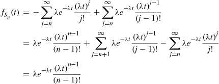
which, upon differentiation, yields

fSn(t)=-∑j=n∞λe-λt(λt)jj!+∑j=n∞λe-λt(λt)j-1(j-1)!=λe-λt(λt)n-1(n-1)!+∑j=n+1∞λe-λt(λt)j-1(j-1)!-∑j=n∞λe-λt(λt)jj!=λe-λt(λt)n-1(n-1)!

Example 5.13

Suppose that people immigrate into a territory at a Poisson rate λ=1 per day.

(a) What is the expected time until the tenth immigrant arrives?

(b) What is the probability that the elapsed time between the tenth and the eleventh arrival exceeds two days?

Solution:

(a) E[S10]=10/λ=10 days.

(b) P{T11>2}=e-2λ=e-2≈0.133. ■

Proposition 5.1 also gives us another way of defining a Poisson process. Suppose we start with a sequence {Tn,n⩾1} of independent identically distributed exponential random variables each having mean 1/λ. Now let us define a counting process by saying that the nth event of this process occurs at time

Sn≡T1+T2+⋯+Tn

The resultant counting process {N(t),t⩾0}^∗ will be Poisson with rate λ.

Remark

Another way of obtaining the density function of Sn is to note that because Sn is the time of the nth event,

P{t<Sn<t+h}=P{N(t)=n-1,oneeventin(t,t+h)}+o(h)=P{N(t)=n-1}P{oneeventin(t,t+h)}+o(h)=e-λt(λt)n-1(n-1)![λh+o(h)]+o(h)=λe-λt(λt)n-1(n-1)!h+o(h)

where the first equality uses the fact that the probability of 2 or more events in (t,t+h) is o(h). If we now divide both sides of the preceding equation by h and then let h→0, we obtain

fSn(t)=λe-λt(λt)n-1(n-1)!