CHAPTER 9
Black‐Scholes‐Merton Model
The objective in this chapter is to develop a deep and, most importantly, intuitive, understanding of the seminal contributions to option pricing made by Black and Scholes (1973) and Merton (1973). In essence, the BSM approach made mathematical modeling assumptions that allowed the authors to derive a functional form for the option valuation function, namely  .1
.1
Even though it has long been established that real markets deviate substantially from BSM formula, their model still provides the building blocks for the pricing of FX options and valuable insight into how to trade them. For example, we have seen in previous chapters that traders use  in many contexts. Despite the presence of smile directly contradicting the BSM model, traders prefer to perturb the BSM model by making
  a function of
  , than to discard it.
I split the study of BSM into two parts. This chapter studies the derivation of  and provides its functional form. Until now, we have assumed that interest rates are zero. This chapter introduces interest rates into our analysis.
In Chapter 10 I discuss the many equations that follow from  . I provide the functional forms of the Greeks delta, gamma, theta, vanna, and volgamma. I also provide some overdue definitions such as that of the ATM strike.
9.1 THE LOG‐NORMAL DIFFUSION MODEL
The BSM model makes the mathematical assumption that  follows

where  is the so‐called drift term, and
  is a Brownian motion. Perhaps the easiest way to understand this equation is through discretizing it. To do the discretization accurately, we have to apply Ito's Lemma to Equation (9.1). Readers unfamiliar with Ito's Lemma may refer to, in order of increasing detail, Hull (2011), Shreve (2000), or Duffie (2001). However, I urge even readers unfamiliar with Ito's Lemma and who do not wish to consult a separate text to plough on. The main challenge here is conceptual, not technical.
The discretized version of the previous equation is
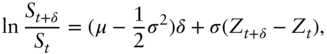
where  is a period of time.
  is a normally distributed random variable with variance
  .
.  is the volatility.
First, set  year. Note that
  is of the order of 10% in FX markets. Therefore,
  is typically small (
 ). I therefore ignore
  for now. Equation (9.2) then says that the annual return of spot is
  plus some randomness. If
  , then the log return would be
  . In reality,
  and so only the expected return is
  .
.
BSM originally wrote this equation with the intention of valuing equity options. The post–World War II average annualized return of the S&P 500 index is approximately 8%. For the S&P equity index at least, one can imagine  to be the right order of magnitude. However,
  is a quantity that is notoriously difficult to estimate. Fortunately, we shall see that one does not need to know
  to price options. Indeed, this was one of the main insights stemming from the BSM approach.
9.2 THE BSM PARTIAL DIFFERENTIAL EQUATION (PDE)
BSM assumes that  is fixed. The value of an option is therefore given by
  and
and  is a parameter. I continue from Equation (2.7) in Section 2.6. Recall that we had considered a portfolio consisting of an option and short an amount
  of the underlying currency.
First, I rewrite Equation (2.7) in differential form. I also apply Ito's Lemma to add in the further terms that I had left out earlier:

Recall also from Chapter 2 that a delta‐hedging trader holds 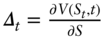 . At this stage, we do not know the functional form of
  , but we will shortly, and therefore the assumption that the trader is able to hold
  of the underlying will be justified. This assumption means that term 2 disappears.
  would have entered through the term
  but it has been eliminated with term 2.
Finally, note that  . I provide some intuition behind this result in the feature box.
Equation (9.3) therefore becomes

The important point to note here is that there is no longer any uncertainty. All of the uncertainty in the BSM model came from the Brownian motion  term, but through delta hedging, the trader has removed it.
One may argue that this uncertainty has only been removed for an instant of time. The idea in the BSM model, however, is that the trader rebalances her deltas continuously in time. That is, an instant of time  later, she adjusts her
  so that she has removed the uncertainty once more. She gamma trades in continuous time. In real markets, traders rebalance at discrete instants of time, rather than continuously. Therefore, there remains some uncertainty and this leads to PnL variance. Nevertheless, at this stage, let us continue to understand the BSM argument by assuming that continual and costless rebalancing is possible.
Suppose that interest rates are zero. This implies that  . This can be understood as follows. First, suppose that
  . If this were true, then one could simply borrow without cost to finance the portfolio
  , and make an arbitrage profit2 over the time period
  . Similary, if
  , then one could make an arbitrage profit over the time period
  by shorting the portfolio
  .
.
In the case of zero interest rates, Equation (9.8) can be written as

Substituting Equations (3.1) and (4.2) we have

This is the famous BSM partial differential equation (PDE) written in perhaps its simplest form. Again, let us take EUR‐USD as our example. The left‐hand side is the theta measured over an instant of time, in EUR. The right‐hand side is the trader's gamma measured in EUR multiplied by volatility  . The equation tells us that gamma and theta can be mapped from one to the other, simply by multiplying by
  .
.
More generally, interest rates are not zero. Let  represent the continuously compounded interest rate in the base currency, namely EUR in the example of EUR‐USD, and let
  represent the continuously compounded interest rate in the numeraire currency, namely USD in the example of EUR‐USD. Suppose also that the trader does not face borrowing or lending transaction costs or constraints.
Assume that the trader starts without any investment capital. She must finance her entire position. In order to finance the portfolio  , she must borrow an amount
  . The cost of this is
  over the next increment of time. She must also borrow
  of the base currency (e.g. EUR) in order to short sell it if she is hedging a call option position. Her cost is
  . For there to be no arbitrage, after the time period
  the trader must still have zero capital, because there is no risk. Therefore the following equation must hold true:

Rearranging and tidying up gives us the full BSM PDE:

In the case of a call option, the boundary condition is  and it is
 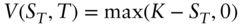 for a put option.
Earlier, I discussed borrowing EUR to short sell. This is true in the case of a call option. In the case of a put option, one would borrow USD and short sell. However, Equation (9.10) looks the same.
There are several methods that one can use to solve this PDE in order to calculate explicitly  (see Shreve, 2000). The solution turns out to be

 is the standard normal CDF.
  for a call option and
  for a put option. Now that we have the solution, I have labeled
  as
as  and
and  as
as  .
.
Next, I show the reader how to relate this PDE back to our studies in the early chapters of this text. This is the topic of the next section.
9.3 FEYNMAN‐KAC
Feynman and Kac showed that the PDE in Equation (9.10) is equivalent to calculating the following expectation for a call option,

where

I do not re‐derive the Feynman‐Kac solution here and I refer interested readers to Duffie (2001) for a rigorous analysis. However, the equivalence between (9.12) and (9.10) is intuitive. Equation (9.12) clearly satisifes the boundary condition 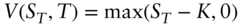 . As long as the left‐hand side is a function of
  and
and  only, then we can apply the logic of the previous section and Ito's Lemma to show that
  satisfies Equation (9.10).
It is important to understand the main implications of Equation (9.12). First, note that it is almost identical to Equation (2.2) but for two main differences.
First, the previous equation contains  explicitly and
  implicitly via
  . In Chapter 2 we set interest rates to zero and therefore these parameters do not appear in Equation (2.2).
The second difference is more subtle, but also more important. It relates to the probability measure under which the expectation is taken. This is the topic of the next section.
9.4 RISK‐NEUTRAL PROBABILITIES
Consider the case of zero interest rates again. In Equation (2.2) the reader was led to believe that the expectation was taken under an objective probability measure. By this I mean that the trader uses Equation (9.1) and a value for  based on a forecast or empirical work to calculate
  and value the option. For example, in the case of an option on the S&P 500 index, one may be tempted to use
  based on historic data. Such an approach would lead traders to value ATMS call options higher than ATMS put options, because spot is expected to rise at 8% per year.
However, note that the BSM valuation equation, Equation (9.12), does not even contain  . Recall that we removed it by setting
  . Therefore, even though the trader expects that
  will appreciate at 8% per year, she values the ATMS call at the same price as the ATMS put.
One can understand this as follows. Suppose that a market participant purchases a 1‐year call option with the objective expectation that  will rise by 8% over the next year. The option trader sells the call option and then delta hedges by purchasing the underlying spot. By purchasing the exact amount of spot as her hedge that the option is exposed to, namely
  , she is able to make back what she loses on the option position. Hence, for the seller
  does not matter.
Perhaps a clearer way of seeing this is via put–call parity. Again, assume zero interest rates. The trader sells the ATMS call and buys the ATMS put. Since the BSM model prices the ATMS call and put at the same price, her cost for setting up this portfolio is zero. Simultaneously, the trader purchases spot in notional equal to the options. Clearly, her PnL is zero everywhere, even if spot appreciates at a rate of 8% per year.
The key point to note is that delta hedging removes any exposure to spot. Exposure to interest rates remains because implementing delta hedging involves borrowing and lending. Delta‐hedged options therefore expose the traders to volatility only.
9.5 PROBABILITY OF EXCEEDING THE BREAKEVEN IN THE BSM MODEL
Recall that in Section 6.5 I calculated that the probability that spot exceeds the breakeven of an ATMS straddle was 42% in the context of the normal model. The feature box shows that the same result is approximately true in the context of the BSM model.
9.6 TRADER'S SUMMARY
- BSM is a log‐normal diffusion model.
- The key idea is to construct a risk‐free portfolio by delta hedging continuously in time. This leads to the famous BSM PDE.
- The BSM PDE shows that gamma and theta can be mapped to each other via the volatility.
- The Feynman‐Kac theorem shows us that the price of an option is the expectation of its payoff, as discussed in Chapter 2. However, importantly, this expectation is taken under a risk‐neutral rather than objective probability measure.