CHAPTER 3
The Basic Greeks: Theta
The Greeks are a set of quantities that describe the sensitivity of the price of an option contract to changes in the values of the parameters or variables upon which that contract depends. We already met one of the Greeks in the previous chapter, namely delta  . There, the variable was the spot level.
More precisely, the Greeks are partial derivatives (in the calculus sense) of the option value with respect to variables such as time, the spot level, and the level of volatility, among others. They are the most important quantities to understand for practical options risk management.
One of the main advantages of thinking in terms of Greeks, rather than thinking about the dynamics of individual options, is that Greeks are additive. Consider  . If the trader owns
  options, each with delta
  , then the amount of spot that the trader must transact in the market to be delta hedged is simply minus the sum of the deltas arising from each individual option, −
 . The trader's risk management system is able to aggregate the
  from each option, leaving the trader with just one net number of concern to manage the
  of her entire portfolio.
Arguably the most important Greeks for practical trading are theta, delta, gamma, and vega.1 We studied delta in our model‐free framework in Chapter 2. However, theta, gamma, and vega can also all be understood before resorting to a formal mathematical model. This chapter focuses on theta.
In short, theta refers to the amount of value that an option loses over a short period of time if  and
and  remain unchanged. In practical trading, this period is usually of the order of one day, or less. Option traders typically maintain high awareness of their theta numbers. If a trader a purchases an option, then her theta will be negative and she is said to be paying theta or time decay because the value of an option diminishes as time progresses. If the trader is short an option, then she is said to be earning theta or earning time decay. I return to these points in more detail ahead.
3.1 THETA, 
Section 2.10 introduced the concept of time value  . The main idea was that, for a given level of
  , the value of an option is greater than its intrinsic value;
  , for
, for  . Equivalently, for a given level of
  , the value of an option diminishes over its lifetime.
  and theta,
  , are very closely related. Time value is the amount of value that an option loses over its lifetime for a given level of
  and
and  , whereas theta is the amount of value that an option loses over a short period of time for a given level of
  and
and  . Clearly, the sum of (minus) the theta at every non‐overlapping unit of time between the present time and expiry must equal the time value.
In formal mathematical option models, theta is expressed over an instant of time,

In practice, traders think of theta as the value that an option loses over a discrete period of time, often of the order of a day. This could be the next 24 hours, between the present time and 10 a.m. New York time the next day when most FX options expire, or another analogous variation. There is no fixed convention across risk management systems. Traders typically refer to this quantity as their overnight theta. I provide some examples of overnight theta calculations in the context of ATM options in Section 3.1.1.
The change in option value over a discrete period of time  for a given level of spot
  is
is

This quantity is commonly refered to as an option's time decay over period  to
to  . If the period
  covers the remaining lifetime of the option,
  , where
  is the expiry time, then the time decay is equal to (minus) the time value.
Readers should note the sign convention here, which is to state time value as a positive number and time decay as a negative number. One can almost always avoid ambiguity here by maintaining the logic that option values diminish over time, all else being held constant.
Time value and theta are related as follows,

In our model‐free framework, we can state that  is a negative number because Jensen's Inequality (Section 2.10.1) taught us that options have positive time value. If we assume that
  does not change sign over time, then we can state that
  is negative.
3.1.1 Overnight Theta for an ATM Option
The price of an ATM call option or put option as a percentage of its notional is given approximately by
Here,  is the number of days until expiry of the option. So, for example, an option that expires in 1 week that has a
  has a price of
  . If the notional of the option is 100 million EUR and EUR‐USD is trading at 1.37, then its cash price is 550 thousand EUR, or 753.5 thousand USD. I discuss where this equation comes from in more detail later and ask the reader to take it as given at this stage.
If the spot rate remains unchanged, then one day later, the price of the option is  . In our example, the option has 6 days left to expiry, and it is valued at 704 thousand USD. The trader's overnight theta for a 1‐week ATM option at
  is therefore 49.5 thousand USD.2
More generally, for an ATM call or put option we can write

where  is the notional of the option.3 Here,
  is in the units of
  . If
. If  is measured in USD, for example, then
  is also measured in USD. Overnight theta is then given by

Recall Equation (1.3) provided the breakeven of an ATM straddle. Readers will note the similarity between Equations (1.3) and (3.3). To get from (3.3) to (1.3) is straightforward. From (3.3) the cost of purchasing the straddle is  percent because the trader must purchase both the call and the put. The underlying spot must move by a percentage amount equal to this cost to breakeven; hence Equation (1.3).
Next, let us discuss where Equation (3.3) comes from. It is a special case of the BSM formula applied to an ATM option with zero interest rates. Recall that it is true by definition because  is set such that Equation (3.3) matches the market price of the option. However, in the feature box in Section 3.1.3 I assume that spot follows a normal distribution with standard deviation given by
  and show that such a model provides the same valuation equation.
I urge the reader to memorize Equation (3.3). The reason is that market participants usually quote prices in terms of  . This equation allows a trader to quickly and conveniently calculate approximate option prices and (equivalently) breakevens as well as overnight theta with some mental arithmetic, rather than using option pricing software.
3.1.2 Dependence of  on
on 
The maximum absolute value of  occurs when
  is close to
  . Since it is understood that
  is negative, henceforth I refer to the point of maximum absolute
  simply as the maximum or peak
  .
.
In the BSM model with zero interest rates, the peak value of  occurs when the strike is ATM. That is,
  . However, as discussed in Chapter 1 this means that
  for typical levels of market parameters and for the most liquid expiries (sub 1 year).
Deep ITM and OTM options have much smaller values of  associated with them than ATMS options. Figure 3.1 illustrates the dependence of
  on
on  .
.
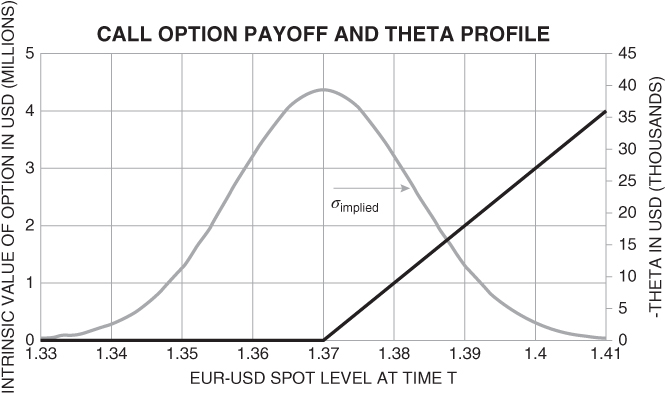
FIGURE 3.1 The figure shows  for a call option with
  and notional of 100 million EUR. Here,
  and the option has 1 week to maturity. The peak theta occurs at
  . At this point, if
  is at 1.37 in 24 hours, then the owner of the option loses about 39 thousand USD in option value in this example.
The idea that the maximum of  occurs at
  is intuitive. Remember, it is the convexity of the payoff that gives options their time value (Section 2.10), and therefore it seems likely that
  will peak at the point of greatest payoff convexity, namely
  and will diminish when
  is far from
  . Let us analyze this in more detail.
Deep OTM Options First, consider a deep OTM call option,  . In short, I argue here that since a deep OTM option has very little value to start with, it has little value to lose over its lifetime and therefore
  is small.
Figure 3.2 shows the PDF and payoff of the situation where  . Almost all of the PDF is over the part where the option payoff is zero. There is only a very small implied probability that
  and that the option pays out at all. Even if the option does payout it is likely that the payout is small. Therefore,
  is close to zero. Since
  when
when  , we see that the left‐hand side of Equation (3.2) is close to zero.
  is negative for all time points,
  , and so it must be true that
  is also small for all
  . If this were not true, then
  would deviate substantially from zero.
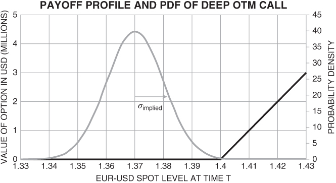
FIGURE 3.2 The figure shows the PDF and payoff profile for a deep OTM option. The probability that the payoff is greater than zero is very small and therefore the option value  is small. If
  remains unchanged, then the option goes from having a low value to zero value. Its
  must therefore be small for all time points
  .
.
Deep ITM Options Next, consider the case of a deep ITM call option,  . Figure 3.3 shows the PDF and payoff of this situation. Almost all of the PDF is over the part where the option is ITM. There is only a very small probability that
  . In short, I argue here that, since the probability that
  is small, the convexity of the option payoff that gave the option its time value (Section 2.10) becomes largely irrelevant and the value of the option is close to its intrinsic value.
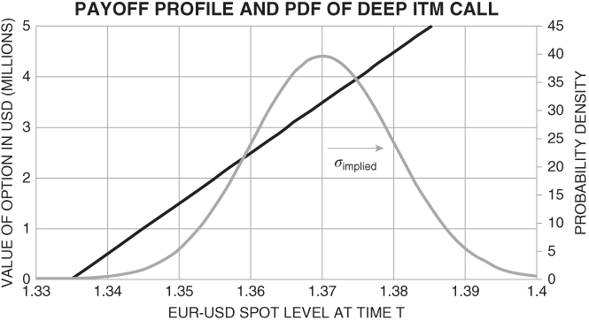
FIGURE 3.3 The figure shows the PDF and payoff profile for a deep ITM option. The PDF lays over the part of the payoff where the option is ITM. The convexity of the option payoff that gave the option its time value becomes less relevant.
To understand this, recall Jensen's Inequality from Section 2.10.1. First, consider the simple case where  can take just two values,
  with probability 0.5 and
  with probability 0.5. Applying our valuation equations from Chapter 2 we find that

Here, I have used strike  . Since the probability that
  is very small for a deep ITM option, I have assumed that the two possible values of
  are above
  .
.
We see that  is equal to its intrinsic value
 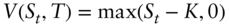 of 3 USD. Applying Equation (3.2), we see that the time value of the option is zero and therefore, since
  is negative for all time points
  , it must be true that
  is also always zero. The key point that this simple example illustrates is that if there is zero (or small) probability that spot crosses through the strike, then the convexity of the option payoff becomes irrelevant and so
  is zero or small.
Next, let us understand the same concept using trading intuition in an analogous manner to Section 2.10.2. Suppose that  and
and  , and the probability that
  is small enough to say that it is essentially zero.
Assume that the trader owns the option with notional 100 million EUR and that she sells 100 million EUR spot as her delta hedge. Her payoff is now 3 million USD with almost certainty. The reason is that, if spot stays in the same place, then the option pays out 3 million USD. If spot goes higher, then for every USD the trader makes on the option, she loses the same amount on her delta hedge. If spot goes lower, with every USD she makes on her spot trade, she loses the same amount on her option position. Crucially, and unlike in Section 2.10.2, there is zero probability that spot moves through the strike. She therefore cannot make more than 3 million USD using this strategy.
The important point here is that the above implies that the value of the option is 3 million USD. The value cannot be less because we have shown in the previous paragraph that there is a simple strategy that locks in 3 million USD; a rational trader will not sell the position for less. The value cannot be more because, if it were, then the trader could simply short sell the call option for an amount greater than 3 million USD and apply the strategy of being short the option and purchasing 100 million EUR as a delta hedge, and receive a payout of 3 million USD with certainty to generate an arbitrage profit.
The value of the option of 3 million USD is equal to its intrinsic value. Again, as was the case for deep OTM options, the left‐hand side of Equation (3.2) is zero and since  is negative for all time points,
  , it must be true that
  is zero for all time points
  . The feature box shows this result more formally.
The important point to note is that for both deep OTM and deep ITM options, the fact that the probability that  moves through the strike
  is zero (or small) means that the convexity of the option payoff is irrelevant and the time value is zero. The reader can work through analogous arguments to those above to show that this is also true for put options.
ATMS Options,  Is at Its Maximum When
  If
If  moves away from
  , the time value of an option diminishes. This happens whether
  moves higher or lower. We already showed earlier that as the option becomes deep ITM or OTM, this time value falls to zero. To establish that
  is the maximum of
  , our task is to show that this diminishing time value as
  either moves ITM or OTM occurs in a monotonic manner. The purpose here is to exclude the possibility that as
  rises (falls),
  increases at some point before falling back to zero as we move deep ITM (OTM). Consider the following two cases.
First, suppose  initially, and then
  falls. The intrinsic value started at zero, and remains at zero for all
  . However, Figure 3.4 shows that the total value of the option diminishes as
  falls. Since the total value of an option is the sum of its intrinsic value and time value, it must be that the time value of the option falls as
  falls.
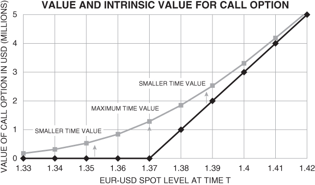
FIGURE 3.4 The gray line shows the option value. The black line shows the intrinsic value. The time value is largest when  . In this case,
  . The time value is smaller as
  moves higher or lower.
Second, suppose  initially, and then
  rises. The intrinsic value started at zero, but then gains at a rate of one for one. That is, if
  moves upward by an amount
  to
to  , then the change in the option's intrinsic value is
  . However, the rise in the total value of the option must be less than
  . The reason is that
  for all values of
  . Recall from Chapter 2 that
  because it is approximately the probability of an ITM expiry and from Figure 2.6 that it is the gradient of the value function. Clearly both of these quantities are less than 1. From the definition of
  , for small
  , the change in value of the option is given by
  . Since the total value of the option rises at a slower rate than the intrinsic value, it must be that the time value falls as
  rises above
  . The next feature box shows these results more formally.
So far I have shown that  falls as
  falls below
  , and that it falls as
  rises above
  . Therefore, the peak in time value must occur when
  . However, our task was to show that
  peaks at
  , not that
  peaks at
  . It is intuitive that the peak in
  occurs close to the same point as the peak in
  . After all, these quantities are closely related in that
  is just the sum (integral) of
  over time. However, we may also obtain the result formally by differentiating Equation (3.6) as shown in the next feature box.
3.1.3 Dependence of  on
on 
The theta of an option is smaller for a long‐dated expiry option than it is for a short‐dated option. For example, if  remains unchanged for say, 1 day, then the decay in the value of a 1‐year expiry option (becoming a 364‐day expiry option) is smaller than the decay on a 1‐week expiry option (becoming a 6‐day expiry option),

That is,  becomes less negative as we extend the maturity or expiry of the option. I described this effect in Section 3.1.1. There, I claimed that the price of an option grows with
  , where
  represents the number of days until expiry. Here, I attempt to provide an intuitive justification for this, and also show that this means that theta bills become less of a concern the longer dated the option expiry.
Consider the following simple approach:

where  ,
,  is the number of days until expiry,
  is the spot value at expiry, and
  is the starting spot value. Readers less familiar with the additive nature of log returns may consult the next feature box.
Assuming that the  are not autocorrelated and are identically distributed, then taking standard deviations on both sides we have that

I provide some evidence that autocorrelations in daily returns are small in Chapter 11. If  represents the annualized standard deviation,
  , then the above equation becomes

The important point to note is that the standard deviation of  grows with the square root of the number of days
  . Therefore, the further that time
  is in the future, the more uncertainty there is about the spot price, as we would expect, but the rate of increase of this uncertainty is diminishing in a square root manner.
Consider a 1‐year option,  days. The standard deviation of the PDF of
  is
is  . One day later, this standard deviation is
  . The change is
Similarly, consider a 1‐month option,  days. The change in the width of the PDF over a day is

Clearly  . The key point is that the standard deviation of the PDF of the spot distribution contracts at a greater rate the shorter time to expiry. Setting
  and so that we can think of time as measured in years rather than days, we have that

which is larger when  is smaller.
To understand how this affects theta, consider Figure 3.5. It shows two PDFs with standard deviations of  and
and  , where
  . By inspecting Figure 3.5 and recalling that the price of the option is equal to its expected payoff (Equation (2.2)), the reader can intuit that the price of the option increases with the standard deviation of the PDF. The longer‐dated option with standard deviation
  has more of the PDF over the area where the option payoff is higher than the shorter‐dated option with standard deviation
  . It is also therefore intuitive that, as 1 day passes, the longer‐dated option decays at a slower rate than the shorter‐dated option, because the standard deviation contracts by
  , which is smaller than
  .
.
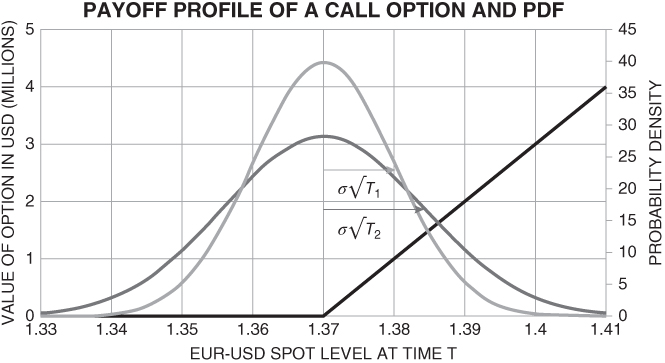
FIGURE 3.5 The figure shows two PDFs, with standard devations of  and
and  , where
  . These overlay the payoff of a 1.37 strike call option. The value of the option is larger for the PDF with
  . The reason is that more of the area under this (wider) PDF is over the area where the payoff of the option is larger.
I make this idea more concrete in the next feature box by showing that the option price is itself linear in  , at least in the context of a normal PDF.
3.2 TRADER'S SUMMARY
- Theta
 represents the amount of value that an option loses over a short period of time if spot remains unchanged.
 - The value of an ATMS call or put option with
 days until expiry is approximately
  .
. - Overnight theta is the amount of value that an option loses in one day. For an ATMS option it can be calculated using Equation (3.5).
- Shorter‐dated options lose value at a faster rate than longer‐dated options. The reason is that the width of the PDF grows in proportion to
 .
. - Deep OTM and deep ITM have little theta. The peak absolute value of theta when an option is (approximately) ATMS,
 .
.
Theta is closely related to another Greek, gamma. In fact, we shall see in Chapter 9 that in the BSM framework one maps to the other via  . Gamma is the topic of the next chapter.