How Will Changes in Population and Income Distribution Affect Global Consumption?
The poorer is a family, the greater is the proportion of the total [expenditure] which must be used for food.... The proportion of the [expenditure] used for food, other things being equal, is the best measure of the material standard of living of a population.
—Ernst Engel
This chapter examines the impact of rising individual incomes on people’s spending choices, by analyzing previous studies and presenting new estimates based on household survey data for 20 economies and 7 consumption categories (food and beverages, transportation, clothing and apparel, housing and equipment, education, health, and other). It then combines these estimates with projections of the global income distribution (reported in chapter 4) to project global consumption for each category. Detailed results are provided for food and beverages (henceforth referred to as “food”) and transportation—the two categories whose shares in total consumption are found to be significantly affected by rising incomes. Chapter 6 examines the implications of the projected changes in consumption for investment in infrastructure.
Because household surveys do not provide income or consumption data by age group, the analysis does not estimate the impact of projected changes in the population’s age structure on consumption choices. It also ignores the impact of consumer demand on prices. The analysis should therefore be viewed as complementary to other efforts to project private consumption and infrastructure needs, which relax some of these assumptions.1
How Do Rising Incomes Affect Individual Economic Choices?
Economists have long studied how changes in a person’s income affect his or her economic behavior, with emphasis on the types of goods and services chosen. In the 19th century, German economist Ernst Engel (1857, 1895) showed that household expenditures on food rise with income and family size but that the share of food in a household’s budgets decreases with income. This relationship, known as Engel’s law, is one of the most robust relationships in economics.2
Constructing “Engel curves” is the first step in projecting global demand for various goods and services. Researchers can do so using data from household surveys or macroeconomic data.
Household-level information provides more accurate projections, for three reasons. First, it permits a more precise analysis of the relationship between total consumption and the share of consumption allocated to a given spending category, because the number of observations far exceeds the number from cross-country comparisons. Second, unlike country averages, household surveys contain information on consumption choices by individuals with relatively low or relatively high incomes. Third, the relationship between a household’s consumption and the share of consumption it allocates to particular types of goods is not always linear; the increase depends on an individual’s income at the beginning of the period. Forecasts of the growth of, say, transportation consumption in a given country therefore depend not only on forecasted changes in the country’s average per capita consumption but also on how income gains are distributed.
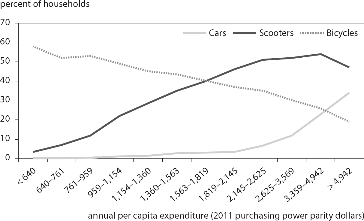
To illustrate the powerful impact of individual’s spending power on consumer choices, figure 5.1 reports the share of India’s population at various levels of total household per capita expenditure who owns a bicycle, a scooter, or a car. As income and consumption rise, people get rid of their bicycles and buy scooters; after their annual expenditure reaches about $2,500, they start buying cars.
People begin purchasing certain consumption goods once they reach various income thresholds. The projections of the number of people whose incomes will exceed those thresholds in 20 years (reported in chapter 4) may thus be interpreted as projections of the number of people who will be able to afford the items listed in table 5.1.
Figure 5.1 Ownership of bicycles, scooters, and cars in India, by level of total household per capita expenditure

Source: Household Consumption of Various Goods and Services in India 2011–12, National Sample Survey 68th round, Ministry of Statistics and Programme Implementation, Government of India, 2014.
Table 5.1 Consumption patterns for different income brackets (international US dollars)

Sources:Chamon, Mauro, and Okawa (2008); Dobbs et al. (2012); Airbus (2015).
As incomes rise, not only do people consume more, they also often shift their spending toward goods that put pressure on natural resources. For example, as their incomes rise, nonvegetarians increase their consumption of meat and fish more than proportionately. These increases contribute to water shortages, overfishing, and climate change.3
Box 5.1 Impact of rising incomes on consumption of “bads”
Consumption of sugary drinks rises rapidly after people can afford a minimally adequate caloric intake; its share in total consumption declines at higher levels of income. Excess consumption of sugared drinks contributes to obesity and rising costs of health care. Cross-country scatter plots of soda consumption versus GDP per capita show a positive and significant correlation, though outliers (such as the United States and Mexico on the positive side and several Asian countries on the negative side) suggest that cultural and other factors are at play (Credit Suisse 2013).
Consumption of alcoholic drinks tends to rise with incomes, beginning as soon as individuals (more often, men) begin to leave extreme poverty. (As a result, beer companies have been among the earliest and most successful manufacturers in many emerging-market economies.) The share of spending on alcohol in total consumption first rises with incom1e, then declines after incomes reach a certain level.
But there are important exceptions to the generally positive association between income and alcohol consumption for people in the middle of the income distribution. The most prominent example was the tragic increase in mortality among Russian men in the aftermath of the collapse of the Soviet Union. Although additional factors may have been at play, it seems that as these men saw their incomes and social structure crumble, they turned to consumption of cheaper and more harmful forms of liquor (Brainerd and Cutler 2005). Similar factors—job losses as well as stagnant or declining incomes and relative status—help explain rising death rates for middle-age white non-Hispanic men in the United States during the past two decades. Drug and alcohol poisoning, suicide, and chronic liver diseases account for the increase (Case and Deaton 2015).
Smoking (of at least one cigarette a day) is prevalent in some of the poorest countries on earth, even among some of the lowest-income groups.1 The poor may even use smoking as an appetite suppressant. One of us once reluctantly agreed to ride in a cycle rickshaw in Indonesia. At noon the rickshaw driver paused for a moment, lit a cigarette, and explained “lunch.” In contrast, in rich countries smoking is less prevalent among high-income groups; education and peer effects may be driving the relationship (Pampel 2010).
1. Data are available from the World Health Organization’s Global Health Data Repository, http://apps.who.int/gho/data/node.main.65.
For some items, people do not necessarily increase consumption when income rises. This is especially evident for tobacco products or for types of food or drink for which it is difficult to draw the line between “goods” and “bads,” such as alcohol and sugared drinks. In such cases, the link with income is often obscured by variation in education, personal sense of selfworth, and stress (box 5.1).
The impact of rising incomes is beginning to be investigated for many important life choices beyond consumption. For example, in developing economies higher incomes increase the likelihood that people migrate. According to research summarized by Michael A. Clemens (2014), throughout the late 20th century the relationship between emigration and real income per capita had an inverted ư-shape, whose curvature became more pronounced over time: In the per capita income range between $600 (that of Niger or Ethiopia today) and $7,500 (Albania or Colombia today), countries with higher per capita incomes experienced more emigration. By the end of the 20th century, richer countries in this range on average had nine percentage points more migration abroad than the poorest countries in the same range.4 For countries with per capita incomes above $7,500, the relationship is reversed. The evidence thus suggests that when people are very poor, rising incomes are more likely to lead them to emigrate but that after they reach middle-income levels further income gains make them less prone to leave their country of origin.
A possible interpretation of this finding is that people living in extreme poverty lack both information on and the means to migrate. In a telling example from fiction, Lila and Lena, 12-year olds in the 1950s Neapolitan impoverished neighborhood depicted by Elena Ferrante in My Brilliant Friend, have never seen the sea—even though their city hugs the Mediterranean.
A back-of-the-envelope calculation based on the individual income projections presented in chapter 4 suggests that the number of people earning $2,000–8,000—who would seem most interested in migrating across national borders, based on Clemens’ (2014) review—is likely to double over the next 20 years, with the largest increases in Sub-Saharan Africa, South Asia, and India. This doubling of the potential pool of migrants suggests that, other things equal, actual migration across national borders is likely to rise significantly from current levels. The extent of the actual increase will depend on a host of factors including conflicts, climate change, and restrictions by recipient countries.
New Estimates of Impact of Rising Incomes on Spending Choices
The estimates presented here focus on how rising incomes affect individuals’ shares of spending on seven categories (food and beverages, transportation, clothing and apparel, housing and equipment, education, health, and other), using data from household surveys for 20 economies.5 This is the first estimation of Engel curves for those categories for a sample of several advanced and emerging-market economies.
The share of spending on each category is regressed on the natural logarithm of total consumption (in 2011 purchasing power parity dollars).6 For each survey, average consumption of each category is calculated for households in each total individual consumption range. Total consumption ranges are defined by narrow, $100 increments (yielding, for example, the $10,000-$10,100 range), to enhance the precision of the estimates. Each of these averages constitutes a data point for estimating the relationship between per capita household consumption and spending on each category of goods and services.
Figure 5.2 shows the negative, broadly linear relationship between the logarithm of total individual consumption and the share of spending on food. The relationship is estimated by pooling all data points for all countries in the sample.7 The results are consistent with Engel’s law.8
Figure 5.3 reveals a positive, more nonlinear empirical association between the logarithm of total individual consumption and the share of spending on transportation in the same economies. The relationship is convex at lower income levels (the share of spending rises more steeply as income grows). It becomes concave at higher income levels (the share of spending rises less steeply as satiation sets in). The fitted relationships in figures 5.2 and 5.3 are estimated using functions (logistic for food and Gompertz for transportation) that allow for the possibility of an S-shape, if warranted by the data.9
Figure 5.2 Estimated Engel curves for food based on household survey data from 20 economies
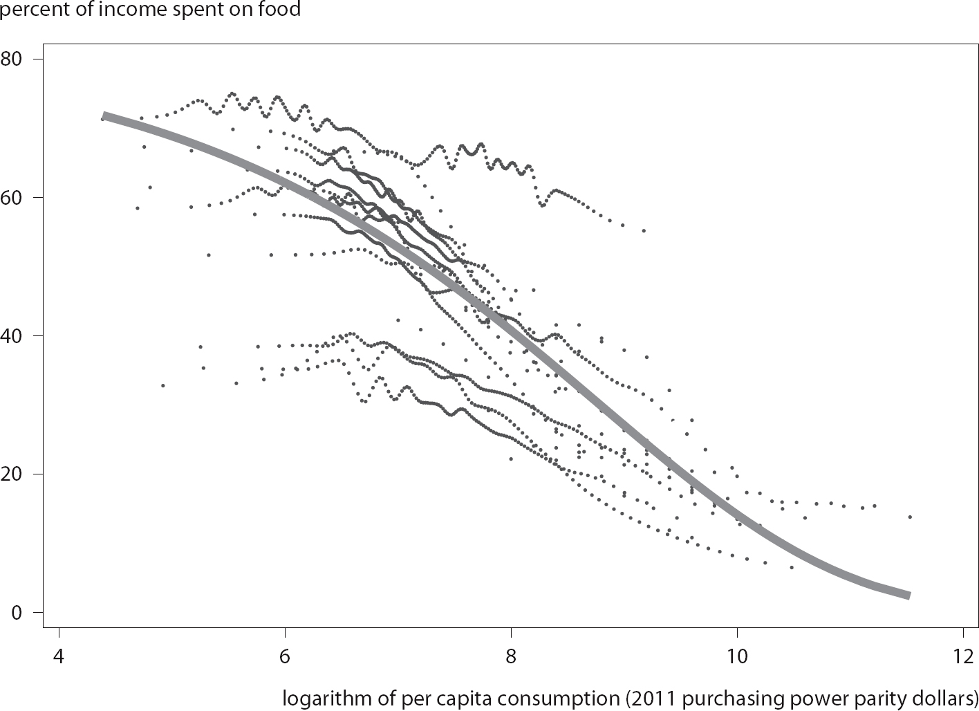
Note: The figure was estimated using a logistic function based on panel data. “Food” includes both food and beverages.
Sources: Data from the World Bank Global Consumption Database, the Luxembourg Income Study, and the Consumer Expenditure Survey (conducted by the US Bureau of Labor Statistics).
Figure 5.3 Estimated Engel curves for transportation based on household survey data from 20 economies
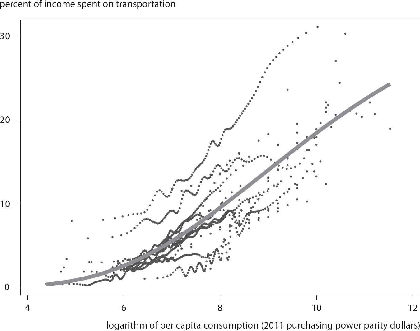
Note: The figure was estimated using a Gompertz function based on panel data.
Sources: Data from the World Bank Global Consumption Database, the Luxembourg Income Study, and the Consumer Expenditure Survey (conducted by the US Bureau of Labor Statistics).
The estimated Engel curves for both food and transportation display strong goodness of fit (adjusted R2 of 0.95 for food and 0.86 for transportation). As in many previous studies, the estimated slope for food is negative and linear for most income levels. At very high income levels, the relationship flattens, becoming nearly horizontal. Table 5.2 shows the estimated coefficients, based on 1,293 observations (each of which is an average of many household-level observations within a narrowly defined range of individual consumption).
The share of transportation spending in total consumption is flat at low levels of total consumption, rises as consumption increases to levels typically associated with advanced economies, and then becomes flatter. The S-shape for total transportation spending is less pronounced (less nonlinear) than in studies of cars alone (Dargay, Gately, and Sommer 2007; Chamon, Mauro, and Okawa 2008), perhaps as a result of two factors. First, households are not able to afford cars when their incomes are below a minimum threshold (estimated by Chamon, Mauro, and Okawa at $5,000 a year based on a panel of countries). Second, in several advanced economies, satiation is observed for car travel at high income levels; it is less likely to affect spending on transportation more generally, including air travel.10
Table 5.2 Estimated Engel curve coefficients for food and transportation based on household
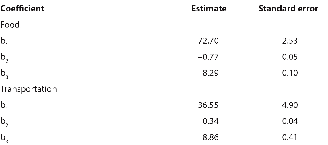
Note: The coefficients for food are based on the logistic model  . The coefficients for transportation are based on the Gompertz model
  .
.
The shares of food and transportation in total spending change significantly as individual incomes rise. People whose total annual consumption is $200 a year spend an estimated 66.3 percent of their total consumption on food and 1.2 percent on transportation. When total consumption reaches $200,000 a year, the figure for food falls to 3.4 percent and the figure for transportation rises to 26.4 percent (table 5.3).
The estimated spending share is also reported for the remaining categories (clothing and apparel, housing and equipment, education, health, and other), based on the corresponding Engel curves (linear).11 In contrast to the estimates for food and transportation, estimates for these categories are not robust to changes in the sample or the estimation technique and are therefore not pursued further.12
Table 5.3 Estimated consumption shares of various categories of goods and services at diferent levels of total annual consumption (shares in percent of total consumption)
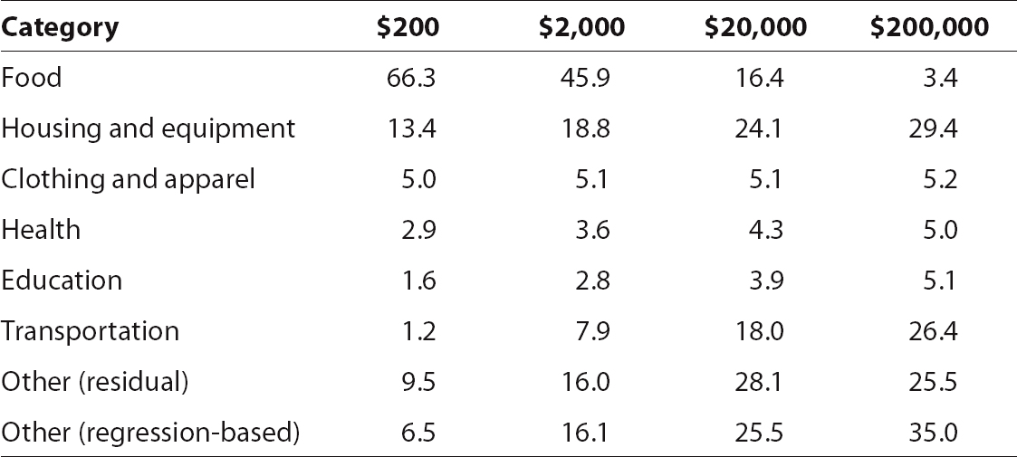
Note: “Other (residual)” is the difference between 100 percent and the sum of the shares of all other categories. “Other (regression-based)” is from the estimated Engel curve for the category “other” in the data.
Source: Data from the World Bank’s Global Consumption Database, the Luxembourg Income Study, and the Consumer Expenditure Survey (conducted by the US Bureau of Labor Statistics).
Projected Spending on Food and Transportation
This section combines two sets of data to project demand for food and transportation by 2035. The first is projections of total consumption at the individual level worldwide, obtained in chapter 4 by combining the individual distribution of incomes (or consumption) within each country in 2015 with projections for each country’s GDP growth between 2015 and 2035. The second is the Engel curves displayed in the previous section. Each individual worldwide is assigned the amount of each consumption category that can be read off the Engel curves at his or her income level. Summing the consumption of each category over all individuals yields category totals for each country and for the world as a whole.
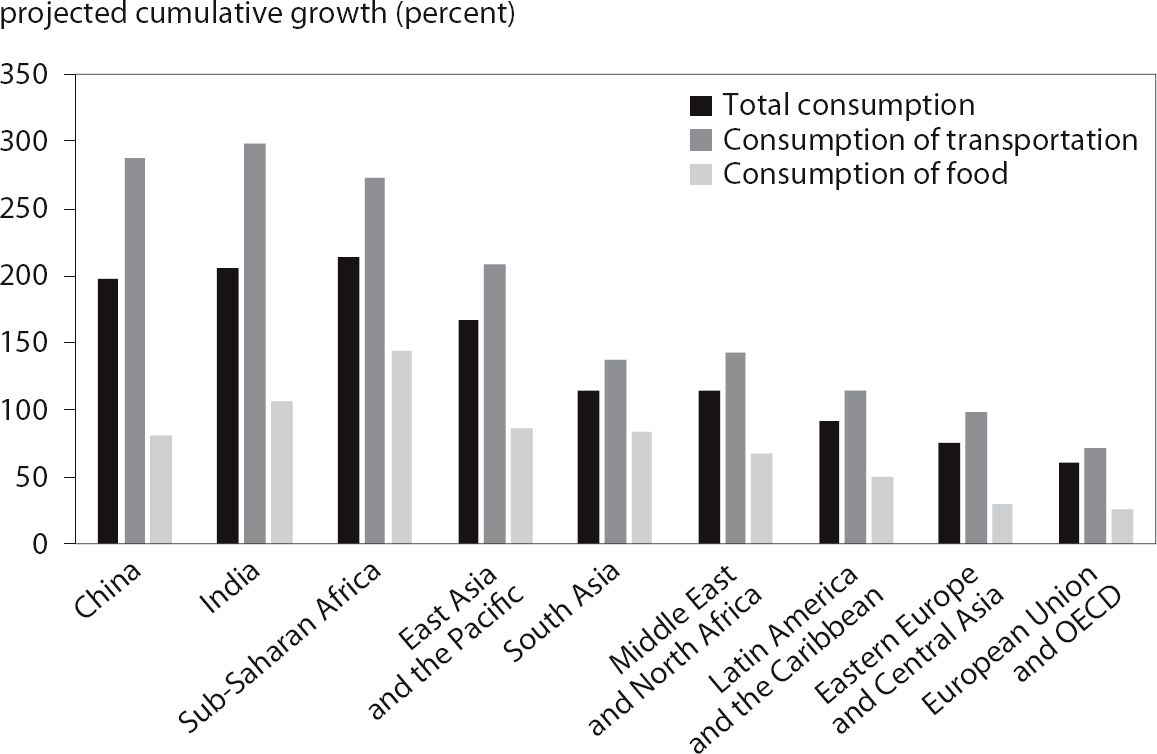
Figure 5.4 Projected cumulative growth in total consumption, transportation, and food between 2015 and 2035, by country and region
Note: Data are in constant prices.
Sources: Data from the World Bank Global Consumption Database, the Luxembourg Income Study, and the Consumer Expenditure Survey (conducted by the US Bureau of Labor Statistics).
Figure 5.4 reports the projected growth rates (in constant prices) between 2015 and 2035 for food and transportation by country or region. Spending on transportation is projected to increase by 300 percent in India, 290 percent in China, 275 percent in Sub-Saharan Africa, 210 percent in East Asia and the Pacific, and 100–150 percent in all remaining emerging-market regions. The increase is projected to be smallest (70 percent) in the European Union (EU)/Organization for Economic Cooperation and Development (OECD) group.
Using the full within-country distribution of individual incomes is valuable, because many individuals are in sections of the Engel curve that are flatter than in the vicinity of average per capita consumption. Had country averages of total per capita consumption been used in conjunction with the micro-based Engel curves reported in figures 5.2 and 5.3, the projected growth rates of transportation consumption would have been considerably higher for all countries and regions—by as much as 60–70 percentage points in India and Sub-Saharan Africa—primarily because the mean individual income in a country’s or region’s total consumption distribution is usually in the steepest section of the transportation Engel curve.
For food consumption, the highest growth rate is projected for Sub-Saharan Africa (145 percent), stemming in part from the rapid growth of total consumption there (the gap between the growth rates of food consumption and total consumption is relatively small, because of the sizable initial share of food in total consumption).13 Total spending on food increases by 110 percent in India and 80–90 percent in East Asia and the Pacific, South Asia, and China. The lowest growth rates for food spending (25–30 percent) are projected for the European Union/OECD, Eastern Europe, and Central Asia.
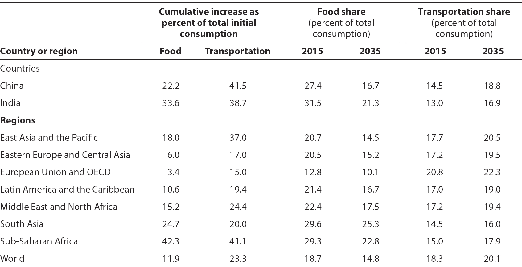
The global share of food is projected to decline to 14.8 percent of total consumption in 2035, down from 18.7 percent in 2015 (table 5.4). The average transportation share in total consumption is projected to rise to 20.1 percent, up from 18.3 percent in 2015. Shifts in consumption patterns vary widely across countries or regions, with larger increases in the transportation share in emerging-market economies.
Table 5.4 also reports the cumulative increase in food and transportation between 2015 and 2035, expressed as a share of 2015 consumption. Higher increases in transportation spending as a share of the initial size of the economy suggest a greater challenge to finance the supporting infrastructure investment. The largest increases are projected for transportation in China (49.9 percent), India (43.6 percent), and Sub-Saharan Africa (42.8 percent).
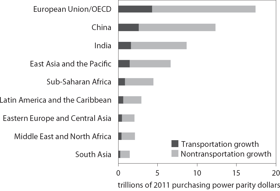
Total consumption and transportation spending will increase more in emerging-market economies than advanced economies over the next 20 years (figure 5.5). Despite slower projected economic growth in the advanced economies, however, they will continue to account for a sizable share of the global increase in both total and transportation spending. Annual consumption of transportation services will increase at an annual rate of 4.2 percent globally and 5.8 percent in non-OECD economies between 2015 and 2035.14 In emerging-market economies, the transportation sector will account for more than a quarter of the increase in total consumption in the next two decades.
Increases in consumption of both transportation and food will raise greenhouse gas emissions and put pressure on natural resources. In the emerging-market economies in particular, the heavier weight of transportation in the total consumption increase suggests a rise in the relative importance of this sector in future greenhouse gas emissions.15 Increased food consumption will also have serious environmental effects. Consumption of meat and fish rise with income. They require more energy and water to produce and yield more carbon dioxide emissions than vegetarian sources of calories and protein. Deforestation, desertification, and overfishing may also ensue, unless measures are taken to keep them in check. Policymakers will need to take these effects into account as they plan for the future.
Table 5.4 Estimated (2015) and projected (2035) spending on food and transportation, by region or country
OECD = Organization for Economic Cooperation and Development
Source: Data from the World Bank’s Global Consumption Database.
Figure 5.5 Projected rise in spending on transportation and nontransportation, 2015–35
Sources: Data from the World Bank Global Consumption Database, the Luxembourg Income Study, and the Consumer Expenditure Survey (conducted by the US Bureau of Labor Statistics).
1. Earlier projections—of spending on transportation (OECD and ITF 2015), energy consumption (IEA 2015), and infrastructure requirements (OECD 2012), for example—use a combination of bottom-up and top-down approaches or multiequation models. Some of these models project demand for various transportation modes (road, rail, ship, air, freight, passenger). These estimates generally do not use the distribution of household incomes within individual countries, however; the assumed relationships between income and spending on specific items are based on cross-country relationships estimated using per capita averages. Moreover, studies usually focus on just one or a few expenditure items rather than on total consumption and its subcomponents.
2. The share of spending on food generally declines linearly with the logarithm of income, although there is evidence of nonlinearity at very high and very low incomes (see Lewbel 2006 for references).
3. Consumption of meat—particularly beef—contributes to emissions of methane, a green-house gas that has a more deleterious effect on the climate than carbon dioxide (Foley 2014, Kunzig 2014).
4. These results would overturn conventional wisdom about the effectiveness of aid to low-income economies as a means of stemming migration flows (Clemens 2014).
5. The estimates include only direct spending by consumers. Food does not include government subsidies. Transportation covers only transit by people, not the transport of goods. The data come from three sources. Data for Albania (2008), Bangladesh (2010), Brazil (2008), Colombia (2010), Indonesia (2010), India (2011), Mexico (2010), Malawi (2010), Pakistan (2010), South Africa (2010), Uganda (2009), and Vietnam (2008) are from the World Bank’s Global Consumption Database. Data for Australia (2010), France (2010), Hungary (2012), Mexico (2010), Poland (2010), Russia (2013), Slovenia (2010), South Africa (2010), and Taiwan (2010 are from the LIS. Data for the United States (2013) are from the Consumption Expenditure Survey (conducted by the Bureau of Labor Statistics). Each survey covers several thousand individuals. Data on Mexico and South Africa come from two surveys. They yield slightly different shares spent on food and transportation at each individual income level, but the patterns are similar. Both the Global Consumption Database and the LIS seek to ensure cross-country comparability of the surveys, including the definition of spending categories.
6. The use of logarithms, which is customary in studies of this kind, makes it more likely that some of the relationships—notably between total consumption and the share of food in total consumption—will be linear.
7. The results are similar if the estimated curves for each country are allowed to have their own intercepts, to reflect any country-specific factors that may influence average consumption of specific categories. (Such factors include any remaining differences in the way the surveys define the categories, despite efforts to make the surveys internationally comparable.) The slope and curvature are estimated under the assumption that they are the same in all countries.
8. More detailed estimates (not reported) show that the share of beverages (especially alcohol and sugary drinks) in total consumption declines more slowly than the share of food. The share of meat and fish in total consumption also declines more slowly than the share of food generally.
9. Both the logistic and the Gompertz function have the potential for two asymptotes (instances in which the relationship becomes flatter and flatter and eventually horizontal), one at very low incomes and the other at very high income levels. The logistic form is symmetric, whereas the Gompertz can be asymmetric. The choice between them was based on goodness of fit and consistency with previous analyses on related topics. For food the logistic function is preferred to the Gompertz function, because it provides slightly better fit and the estimated coefficients imply that although very-high-income individuals reduce their share of food in overall consumption, they continue to increase the absolute amount of expenditure on food as incomes rise. For transportation a Gompertz function is estimated, as in several studies of the market for cars (for example, Dargay, Gately, and Sommer 2007, who estimate a Gompertz function relating average per capita real incomes and the average number of cars in the population for a cross section of countries).
10. Passenger vehicle travel declined in recent years in several advanced economies, notably Japan and the United Kingdom (OECD and ITF 2015).
11. Estimation of the Engel curve for health allows for different intercepts for each country, to reduce the influence of the United States, an outlier with much higher healthcare spending at all income levels.
12. The share of health care in total spending bears no clear relationship to individual incomes, in contrast to the strong positive association between the share of healthcare spending and average GDP per capita documented in studies based on time-series information from macroeconomic data (see, for example, Jones 2015). The absence of an empirical association in the microeconomic data casts doubt on the notion that health is a luxury good (i.e., a good whose demand rises more than proportionately with income), pointing instead to increases in the relative cost of health care over time as a key driving factor.
13. The gap between the growth rates of spending on food (F) and overall consumption (C) equals  . It thus depends not only on the slope of the Engel curve (
 but also (negatively) on the initial ratio of spending category F to total consumpt
14. These projections are higher than some others. The OECD and ITF (2015) estimate that road and rail passenger travel will grow at an annual rate of 2.3–3.5 percent globally and 3.6–5.0 percent in non-OECD economies through 2050.
15. The share of carbon dioxide emissions attributable to transportation in the largest emerging-market economies was less than 10 percent before 2012 (IEA 2015).