Reading Data with a SET Statement
Determining Which Table a Record Is From
Using a SET Statement With KEY=
Determining Whether a Table Exists
Verifying That a Table Has Records
Working with data tables is a fundamental part of SAS, which means there are many programming choices when you need to manipulate data tables. This chapter shows you some techniques that will help you work with data tables.
I often find that I need to make a new table that has the same variables and attributes as an existing table, usually because I’m going to append the new table to the existing table and want the attributes to be the same. You can hardcode all the lengths, formats, informats, and labels for the variables, but this creates a maintenance headache if the original table changes. The technique I use is to add these lines at the beginning of the DATA step:
if (0) then
set table;
Here is how this works:
● When you run a DATA step, the program data vector (PDV) is created at compile time, before any of the code in the DATA step is actually executed. The PDV is a list of all the variables and their attributes that are used during the DATA step. The compiler gathers all these variables from the DATA step code and from the headers of any tables that are referenced in the DATA step. The compile step happens one time before executing the DATA step.
● When you use this technique, the variables and their attributes in the table on the SET statement are brought into the PDV during the compile step.
● When the DATA step is executed after the compile step, and each time it runs the IF statement, it considers the condition to be false (because 0=false in SAS), so it doesn’t execute the statement, or statements, after the THEN. This means that no data is ever read from that table.
● So the variables and their attributes are brought into the PDV by the compiler, but records in the table are never read.
In the example in Program 2.1, I want to create a new table with the same variables and attributes as the sashelp.class table.
Program 2.1: Creating a New Table with the Same Attributes
data newClass;
if (0) then
set sashelp.class;
input name sex age height weight;
datalines;
Susan F 10 50 75
Chris M 10 53 80
;
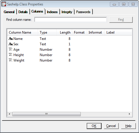
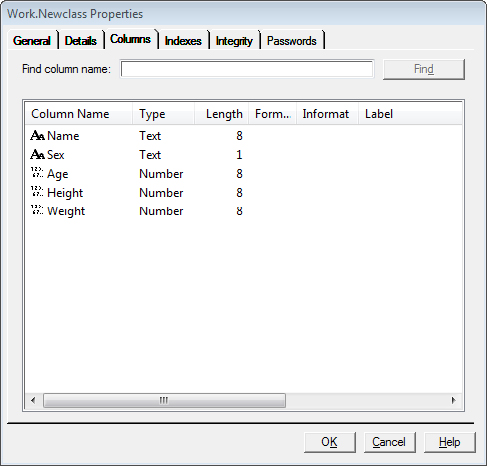
After running the code in Program 2.1, the variables in the newClass table are the same as the ones in the sashelp.class table, as you can see in Figure 2.1 and Figure 2.2.
Figure 2.1: sashelp.class Variable Properties

Figure 2.2: work.newClass Variable Properties
Be sure to put the IF statement close to the beginning of your DATA step; the variables are added to the PDV in the order that the compiler finds them.
Variable lengths can sometimes cause issues when you use this technique. If you use a LENGTH statement before the IF (0) statement, and you specify the length of a variable to be shorter than the variable in the table, then you will get warnings in your SAS log:
data newClass;
length name $4;
if (0) then
set sashelp.class;
input name sex age height weight;
datalines;
Susan F 10 50 75
Chris M 10 53 80
;
This code causes these warnings in the SAS log:
WARNING: Multiple lengths were specified for the variable name by input data set(s). This can cause truncation of data.
If your code is working the way you want, you can temporarily turn off these warnings in your logs with the VARLENCHK= option. You should then turn the warnings back on after the DATA step. I don’t recommend setting the option at the beginning of your code, because there are times that the warning indicates an issue that should be fixed. But if you are sure that the warning is not a problem, you can set the option to NOWARN before the DATA step and then back to WARN after the DATA step as in the example in Program 2.2 and SAS Log 2.1.
Program 2.2: Suppressing Warning Messages
options varlenchk = NOWARN;
data newClass;
length name $4;
if (0) then
set sashelp.class;
input name sex age height weight;
datalines;
Susan F 10 50 75
Chris M 10 53 80
;
options varlenchk = WARN;
SAS Log 2.1: Suppressing Warning Messages
1 options varlenchk = NOWARN;
2 data newClass;
3 length name $4;
4 if (0) then
5 set sashelp.class;
6 input name sex age height weight;
7 datalines;
NOTE: The data set WORK.NEWCLASS has 2 observations and 5 variables.
NOTE: DATA statement used (Total process time):
real time 0.01 seconds
cpu time 0.00 seconds
8 ;
9 options varlenchk = WARN;
Warning: When you use this technique without referencing any other input sources (with SET, MERGE, UPDATE or INFILE statements), then you need to use a STOP statement at the end of the DATA step. Even though the SET statement is not executed, the DATA step still knows that it is there, so the DATA step waits for an end-of-file marker to tell it to stop processing. And since no data is read from an input source, there will never be an end-of-file marker. So you must use the STOP statement to explicitly tell the DATA step to stop processing.
Reading an existing data table into your DATA step is a simple process using the SET statement. You can also use the SET statement to read multiple tables and to read the data out of sequence.
If you want to add multiple tables together, one after another, you can simply list all the tables on a single SET statement. This causes the DATA step to read all the records from the first table, then all the records from the second table, and so on until it has read all the records from all the tables. The tables don’t even have to have the same variables, though usually it is more useful if they do.
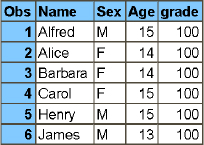
The code in Program 2.3 creates two class tables—one for each year—that are used in the example in Program 2.4. Figure 2.3 and Figure 2.4 show these two tables.
Program 2.3: Creating class Tables
data class_2016;
set sashelp.class (obs = 5);
run;
data class_2017;
set sashelp.class (keep = name sex age
obs = 6);
age + 1;
grade = 100;
run;
Figure 2.3: Creating class Tables—work.class_2016
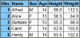
Figure 2.4: Creating class Tables—work.class_2017
You can use a SET statement to concatenate these two tables, even though they don’t have the same variables. The example in Program 2.4 shows how to concatenate the two class tables, and Figure 2.5 shows a listing of the output table. I also use the IN= option to help create a year variable to indicate which table the record came from.
Program 2.4: Concatenating Tables with a SET Statement
data class;
set class_2016 (in = in_2016)
class_2017 (in = in_2017);
if (in_2016) then
year = 2016;
else if (in_2017) then
year = 2017;
run;
Figure 2.5: ConcatenatingTables with a SET Statement
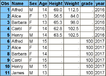
The Height and Weight variables are only in the class_2016 table, so the values are missing on the 2017 records. The grade variable is only in the class_2017 table, so the values are missing on the 2016 records.
If you have multiple tables that are sorted by the same variables, then you can interleave the tables using a SET statement with a BY statement. The records are read in sorted order from all the input tables. Program 2.5 and SAS Log 2.2 show how to interleave a table containing the males in sashelp.class with the females from sashelp.class.
Program 2.5: Interleaving Tables
proc sort data = sashelp.class
out = male;
where sex = "M";
by name;
run;
proc sort data = sashelp.class
out = female;
where sex = "F";
by name;
run;
data _null_;
set male
female;
by name;
putlog name= sex=;
run;
SAS Log 2.2: Interleaving Tables
Name=Alfred Sex=M
Name=Alice Sex=F
Name=Barbara Sex=F
Name=Carol Sex=F
Name=Henry Sex=M
Name=James Sex=M
Name=Jane Sex=F
Name=Janet Sex=F
...
You can see that the records are read in sorted order from both tables, rather than all the records being read from the first table and then all the records from the second table.
You can use more than one SET statement in a single DATA step. If you do this, the DATA step reads a record from the data table each time the SET statement is executed. So if you have two SET statements one after another in the DATA step, it reads a record from the table on the first SET statement and then a record from the table on the second SET statement in the same iteration of the DATA step. This means that you must be careful about the variables in each table so that values from a second table don’t overwrite those from the first table. The other thing to watch out for is the end of file. The DATA step stops iterating when it reaches the end of any file that is being read, so whichever table has the smallest number of records causes the DATA step to stop iterating before all the records in the other tables have been read.
When I use multiple SET statements, I usually use the NOBS= and POINT= options on at least one of the SET statements.
● The NOBS= option creates a variable that contains the number of records in the incoming table.
● The POINT= option points to a variable that you create that contains the record number that is read from the table.
So if you are reading one table, and you want to look up values in a second table, you can use the POINT= and NOBS= options to let you loop through the second table. Using this technique means that you don’t hit the end-of-file condition that stops your DATA step iteration. Even if you read the last record, it doesn’t trigger the end-of-file flag.
Program 2.6 and SAS Log 2.3 are an example of using the POINT= and NOBS= options for looking up values in a second table. Using the sashelp.class table and 10 records from the sashelp.classfit table as a lookup table, you can look up the predicted weight for each person.
Program 2.6: Using POINT= and NOBS=
data classfit (keep = name predict);
set sashelp.classfit (obs = 10);
run;
data _null_;
set sashelp.class;
do p = 1 to nobs; ❶
set classfit (rename = (name = name_fit)) ❷
point = p nobs = nobs;
if (name eq name_fit) then
do;
putlog name= weight= predict= 5.1;
leave; ❸
end;
end;
run;
❶ The p variable is used in the POINT= option and is incremented so that each record of the classfit table is read. The nobs variable is automatically set to the number of records in the classfit table by the NOBS= option.
❷ It is necessary to rename the name variable when reading the classfit table, because the name value from sashelp.classfit overwrites the name value from sashelp.class.
❸ The LEAVE statement causes the execution to exit the DO loop when it finds the match so that you don’t read the entire lookup table for each record in the sashelp.class table. If you are looking for multiple matches, then you would not use the LEAVE statement.
SAS Log 2.3: Using POINT= and NOBS=
Name=Alice Weight=84 predict=77.3
Name=Carol Weight=102.5 predict=101.8
Name=James Weight=83 predict=80.4
Name=Jane Weight=84.5 predict=90.1
Name=Janet Weight=112.5 predict=100.7
Name=Jeffrey Weight=84 predict=100.7
Name=John Weight=99.5 predict=87.0
Name=Joyce Weight=50.5 predict=57.0
Name=Louise Weight=77 predict=76.5
Name=Thomas Weight=85 predict=81.2
I tend to use p as the variable name for the POINT= option, and nobs for the NOBS= option. These are easy to remember. If you are setting multiple tables using the POINT= and NOBS= options, then you should use a different variable for each POINT= and NOBS= option.
The KEY= option enables you to read matching records from a second table using an index. The index must be set up on the second table and the variables included in the index must be set to appropriate values before executing the SET statement with the KEY= option.
Program 2.7 and SAS Log 2.4 use the previous example for POINT= and NOBS=, except this time I’ve added an index to the classfit lookup table so that I can use the KEY= option.
Program 2.7: Using KEY=
data classfit (index = (name)
keep = name predict);
set sashelp.classfit (obs = 10);
run;
data _null_;
set sashelp.class;
set classfit key = name;
if (_iorc_ eq 0) then ❶
putlog name= weight= predict= 5.1;
_error_ = 0; ❷
run;
❶ The automatic variable, _IORC_, is set to a return code when you use a SET statement with a KEY= option. A value of 0 indicates that the record was found.
❷ If you are using a KEY= option, you should always set the automatic variable _ERROR_ to 0 at the end of the DATA step. Otherwise all the variable values are written to the SAS log whenever _IORC_ is not 0.
SAS Log 2.4: Using KEY=
Name=Alice Weight=84 predict=77.3
Name=Carol Weight=102.5 predict=101.8
Name=James Weight=83 predict=80.4
Name=Jane Weight=84.5 predict=90.1
Name=Janet Weight=112.5 predict=100.7
Name=Jeffrey Weight=84 predict=100.7
Name=John Weight=99.5 predict=87.0
Name=Joyce Weight=50.5 predict=57.0
Name=Louise Weight=77 predict=76.5
Name=Thomas Weight=85 predict=81.2
If you want to use the KEY= option to look up multiple records from the lookup table, you need to use the KEYRESET= option. This option indicates when to start at the top of the index and when to read the next value in the index. The KEYRESET= option points to a variable that you should set to 1 when you want to start at the top of the index, and set to 0 when you want to read the next value in the index. The option will very nicely set the variable to 0 each time it reads a record.
The example in Program 2.8 and SAS Log 2.5 looks up all the values associated with a given id value.
Program 2.8: Looking up Multiple Records with KEY=
data lookup (index = (id));
input id $1. value $char10.;
datalines;
1 Pear
1 Peach
1 Banana
2 Apple
3 Grape
3 Lemon
;
data main;
input id $1.;
datalines;
1
2
2
;
data _null_;
set main;
reset = 1; ❶
putlog id= reset=;
do until (_iorc_ ne 0);
set lookup key = id keyreset = reset;
if (_iorc_ ne 0) then
leave;
putlog id= value= reset=;
end;
_error_ = 0;
run;
❶ You must set the reset variable to 1 to force the program to start at the top of the index. If you don’t have reset=1, the program does not find any records when it tries to look up the second id=2 value, because it has already read the one record in the lookup table for id=2.
SAS Log 2.5: Looking up Multiple Records with KEY=
id=1 reset=1
id=1 value=Pear reset=0
id=1 value=Peach reset=0
id=1 value=Banana reset=0
id=2 reset=1
id=2 value=Apple reset=0
id=2 reset=1
id=2 value=Apple reset=0
If you use a SET statement or a MERGE statement with multiple data tables, you can take advantage of the IN= data set option. This option enables you to specify a variable that is automatically set to 1 (true) when the current record comes from that data table, and is set to 0 (false) when the current record does not come from that data table.
Program 2.9 and SAS Log 2.6 show an example of using the IN= option with an interleaving SET statement. Records are read from the tables in the order specified on the BY statement.
Program 2.9: Using IN= with SET Statement
proc sort data = sashelp.class
out = male;
where sex = "M";
by name;
run;
proc sort data = sashelp.class
out = female;
where sex = "F";
by name;
run;
data _null_;
set male (in = inM)
female (in = inF);
by name;
putlog inF= inM= name= sex=;
run;
SAS Log 2.6: Using IN= with SET Statement
inF=0 inM=1 Name=Alfred Sex=M
inF=1 inM=0 Name=Alice Sex=F
inF=1 inM=0 Name=Barbara Sex=F
inF=1 inM=0 Name=Carol Sex=F
inF=0 inM=1 Name=Henry Sex=M
inF=0 inM=1 Name=James Sex=M
inF=1 inM=0 Name=Jane Sex=F
inF=1 inM=0 Name=Janet Sex=F
inF=0 inM=1 Name=Jeffrey Sex=M
inF=0 inM=1 Name=John Sex=M
inF=1 inM=0 Name=Joyce Sex=F
inF=1 inM=0 Name=Judy Sex=F
inF=1 inM=0 Name=Louise Sex=F
inF=1 inM=0 Name=Mary Sex=F
inF=0 inM=1 Name=Philip Sex=M
inF=0 inM=1 Name=Robert Sex=M
inF=0 inM=1 Name=Ronald Sex=M
inF=0 inM=1 Name=Thomas Sex=M
inF=0 inM=1 Name=William Sex=M
The IN= option is particularly useful in the MERGE statement to determine whether the current record came from one or multiple tables. In fact, I rarely use a MERGE statement without also using the IN= option.
The example in Program 2.10 and SAS Log 2.7 shows merging two tables together. One table has all the students from the sashelp.class table who are 13 and older, and the second table has all the students who are 14 and older. This means that some of the records from the 13+ table do not have matches in the 14+ table. Using the IN= option on each table in the MERGE statement enables you to determine whether each record came from both tables or only one table.
Program 2.10: Using IN= with MERGE Statement
proc sort data = sashelp.class
out = thirteen_plus;
where age ge 13;
by name;
run;
proc sort data = sashelp.class
out = fourteen_plus (rename = (age = age14));
where age gt 13;
by name;
run;
data _null_;
merge thirteen_plus (in = in13_plus)
fourteen_plus (in = in14_plus);
by name;
putlog in13_plus= in14_plus= name= age=;
run;
SAS Log 2.7: Using IN= with MERGE Statement
in13_plus=1 in14_plus=1 Name=Alfred Age=14
in13_plus=1 in14_plus=0 Name=Alice Age=13
in13_plus=1 in14_plus=0 Name=Barbara Age=13
in13_plus=1 in14_plus=1 Name=Carol Age=14
in13_plus=1 in14_plus=1 Name=Henry Age=14
in13_plus=1 in14_plus=1 Name=Janet Age=15
in13_plus=1 in14_plus=0 Name=Jeffrey Age=13
in13_plus=1 in14_plus=1 Name=Judy Age=14
in13_plus=1 in14_plus=1 Name=Mary Age=15
in13_plus=1 in14_plus=1 Name=Philip Age=16
in13_plus=1 in14_plus=1 Name=Ronald Age=15
in13_plus=1 in14_plus=1 Name=William Age=15
PROC SQL is a great tool for working with data tables and particularly for joining tables. However, it is not necessarily the best tool all the time, just as DATA step is not always the best tool. I think that PROC SQL is hard to debug. I also don’t find it intuitive to write, because it isn’t the top-down programming that I’m used to. But those issues notwithstanding, I still get a lot of use out of PROC SQL.
There are many ways to join data tables together. Should you use PROC SQL or should you use a DATA step with a merge? Unfortunately, the answer is, “It depends.” I use both methods regularly, depending on the situation. Here are some of my reasons for choosing one method over the other.
Choose PROC SQL in the following situations:
● You are doing a simple join and you don’t want to sort the data first.
● You are joining tables that don’t have the same variables to merge by, or you want to use a more complex way of matching the variables in the tables (not just equals).
● You are joining more than two tables and you have different matching criteria for each join.
Choose a DATA step merge in the following situations:
● You want to keep records on the basis of which table they came from (using IN=).
● You need to do some additional DATA step processing, and you don’t another step to read and write the data again after joining it.
Using PROC SQL to join tables is great because it lets you do the actual join in a much more complex way than a DATA step merge, which is a simple matching of variable values.
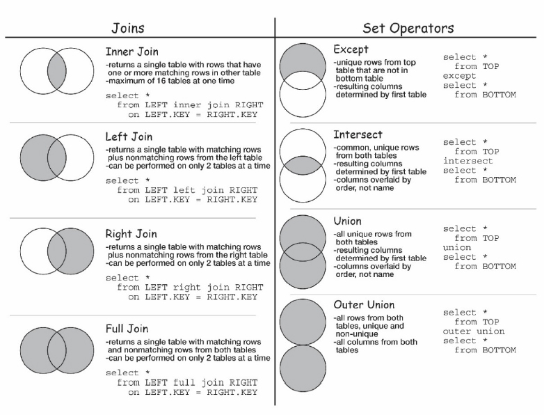
I tend to use the full join, left join, right join, and inner join rather than doing a Cartesian Product join (using a comma between the tables). I can get the same results, and I don’t have to remember when to use a WHERE clause and when to use an ON clause. The cheat sheet in Figure 2.6 can help you to remember what each join does.
Figure 2.6: PROC SQL Join Cheat Sheet
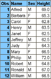
Using subqueries is a great feature of PROC SQL because it enables you to use the output of one query in an expression.
In the example in Program 2.11, if you want to find all the students who are older than the average age in the class, you can do it with a subquery. Figure 2.7 is the output table.
Program 2.11: Using a Subquery to Subset Data
proc sql;
create table tallest as
select name, sex, height
from sashelp.class
where height gt (select avg(height)
from sashelp.class);
quit;
Figure 2.7: Using a Subquery to Subset Data
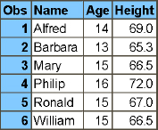
Another good use of a subquery is to compare a value to a set of values from a subquery using the IN operator. For example, the code in Program 2.12 enables you to keep all the students from the sashelp.class table who have the predict value in the sashelp.classfit table greater than 110. Figure 2.8 shows the output table.
Program 2.12: Using a Subquery with an IN Operator
proc sql;
create table predict as
select name, age, height
from sashelp.class
where name in (select name
from sashelp.classfit
where predict gt 110);
quit;
Figure 2.8: Using a Subquery with an IN Operator
A correlated subquery is a subquery that refers to the parent query in the WHERE clause. This means that the subquery is run for each row of the parent query, so it is relatively inefficient.
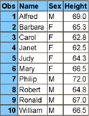
Program 2.13 is an example of a correlated subquery that finds all the students who are taller than the average height by sex. So it compares each girl’s height to the average of all the girls’ heights, not to the average of all the heights. Figure 2.9 is a listing of the output table.
Program 2.13: Using a Correlated Subquery
proc sql;
create table tallest as
select name, sex, height
from sashelp.class as c
where height gt (select avg(height)
from sashelp.class
where sex eq c.sex);
quit;
Figure 2.9: Using a Correlated Subquery
Often in SAS you need to look up values from another table. For example, you might have a table that has userids in it, and you need to get the associated user name from a lookup table. There are lots of ways to do this based on what you are looking up and how big your tables are.
You can create a user-defined format to use if your lookup table meets the following criteria:
● It is a manageable size (you’ll have to determine this by creating the format and seeing whether it takes too long to create and use or takes up too much disk space).
● It has only a couple of variables whose values you want to retrieve (you’ll need a separate format for each variable).
● It has only one value to be retrieved for each lookup value.
The example in Program 2.14 and SAS Log 2.8 uses the sashelp.cars table and illustrates creating a lookup format of each car model to the make of car and a second format of car model to the type of car.
Program 2.14: Using Formats to Look Up Values
data fmtdata (keep = fmtname start label); ❶
set sashelp.cars;
start = left(model);
fmtname = "$make";
label = make;
output;
fmtname = "$type";
label = type;
output;
run;
proc sort data = fmtdata nodupkey; ❷
by fmtname start;
run;
proc format cntlin = fmtdata; ❸
run;
data _null_; ❹
length model $50.;
do model = "MDX", "ABC", "G500";
type = put(model, $type.);
make = put(model, $make.);
putlog model= type= make=;
end;
run;
❶ Create the table needed for PROC FORMAT. It must have a variable called fmtname that contains the name of the format, a variable called start that is the lookup variable’s value, and a variable called label that contains the value to be retrieved.
❷ Group the data by fmtname if you are creating more than one format. You can have no duplicate lookup values (start). I handle both these requirements with a PROC SORT by fmtname and start and the NODUPKEY option.
❸ Run PROC FORMAT with the CNTLIN= option to create the format.
❹ Use a DATA step to test the formats. "ABC" is not a valid model, so it will not replace the model with the make and type.
SAS Log 2.8: Using Formats to Look Up Values
model=MDX type=MDX make=MDX
model=ABC type=ABC make=ABC
model=G500 type=G500 make=G500
See Also: There is a utility macro in Appendix A called %_MAKE_FORMAT() that you can use to create a format from a data table.
Another way to use a lookup table is to join your primary table with the lookup table. This can be done with either PROC SQL or with a DATA step and merge. You can use a join when your lookup table meets these criteria:
● It is any size.
● It has one or more values to be retrieved.
● It has one or more retrieval values per key (though this can be awkward because multiple records are created if there are multiple retrieval values).
The example in Program 2.15 and SAS Log 2.9 uses the sashelp.cars table as a lookup table and a straightforward DATA step to merge the data. Use the IN= option to keep only the records that come from your primary table.
Program 2.15: Using a DATA step Merge to Look Up Values
data primary; ❶
input model $char50.;
datalines;
MDX
ABC
G500
;
data lookup; ❷
set sashelp.cars;
model = left(model);
run;
proc sort data = primary; ❸
by model;
run;
proc sort data = lookup;
by model;
run;
data _null_; ❹
merge primary (in = inP)
lookup;
by model;
if (inP);
putlog model= make= type=;
run;
❶ Create some test data for the primary table.
❷ Fix the cars data: Left-justify the model.
❸ Sort the data so that it can be merged.
❹ Merge the tables and keep only the records from the primary table using the IN= variable.
SAS Log 2.9: Using a DATA step Merge to Look Up Values
model=ABC Make= Type=
model=G500 Make=Mercedes-Benz Type=SUV
model=MDX Make=Acura Type=SUV
Using PROC SQL is even easier than the DATA step, because you don’t need to sort the tables. Also, in this example, you don’t need to fix the model value in the lookup table. Program 2.16 uses a left join to ensure that you keep all the records from your primary table. The output table is listed in Figure 2.10.
Program 2.16: Using PROC SQL to Look Up Values
data primary;
input model $char50.;
datalines;
MDX
ABC
G500
;
proc sql;
create table final as
select p.model, l.make, l.type
from primary as p
left join
sashelp.cars as l
on p.model eq left(l.model);
quit;
Figure 2.10: Using PROC SQL to Look Up Values

In a DATA step, you can also use a SET statement with a KEY= option to retrieve your values from the lookup table. To use this method, your lookup table must meet these criteria:
● It can be any size.
● It has one or more values to be retrieved.
● It has an index on the variable(s) that match the variable name(s) in the primary table.
The example in Program 2.17 and SAS Log 2.10 uses the sashelp.cars table as the lookup table and a SET statement with the KEY= option to look up values.
Program 2.17: Using SET with KEY= to Look Up Values
data primary; ❶
input model $char50.;
datalines;
MDX
ABC
G500
;
data lookup (index = (model)); ❷
set sashelp.cars;
model = left(model);
run;
data _null_; ❸
length make $13 type $8;
call missing(make, type);
set primary; ❹
set lookup key = model;
if (_iorc_ eq 0) then ❺
put "success: " model= make= type=;
else
put "failure: " model=;
_error_ = 0; ❻
run;
❶ Create some test data for the primary table.
❷ Fix the cars data: Left-justify the model. Add an index to the table.
❸ Run a DATA step to look up the values.
❹ Use one SET statement for the primary table and another SET statement with a KEY= option for the lookup table.
❺ Check the _IORC_ automatic variable to see if the value was found in the lookup table or not. A value of 0 means that it was found.
❻ Whenever you use a SET statement with a KEY= option, a MODIFY statement, or any other statements that cause the _IORC_ variable to be created, you should set the _ERROR_ automatic variable to 0. If you don’t do this, the DATA step puts out all the variable values in the log every time the _IORC_ value is not 0.
SAS Log 2.10: Using SET with KEY= to Look Up Values
success: model=MDX make=Acura type=SUV
failure: model=ABC
success: model=G500 make=Mercedes-Benz type=SUV
If you have multiple records for each key value, you can use the same code and loop through the retrieved values instead of just reading one value. The code in Program 2.18 and SAS Log 2.11 shows how to do this.
Program 2.18: Using SET with KEY= to Look Up Multiple Values
data primary; ❶
input make $char50.;
datalines;
XYZ
Mercedes-Benz
Audi
;
data lookup (index = (make)); ❷
set sashelp.cars;
model = left(model);
run;
data _null_;
length model $40 type $8;
call missing(model, type);
set primary; ❸
reset = 1;
do until(_iorc_ ne 0); ❹
set lookup key = make keyreset = reset; ❺
if (_iorc_ eq 0) then ❻
put make= model= type=;
end; /* do until - loop though matching rows */
_error_ = 0; ❼
run;
❶ Create some test data for the primary table.
❷ Fix the cars data: Left-justify the model. Add an index to the table.
❸ Set the primary data table.
❹ Loop through the lookup table to retrieve all matches.
❺ Set the lookup table with the KEY= option pointing to the index. Use the KEYRESET= option to tell the SET statement to go to the next record in the table. Set the reset variable to 0 before the loop begins to tell the SET statement to read the first matching record.
❻ Whenever you use a SET statement with a KEY= option, a MODIFY statement, or any other statements that cause the _IORC_ variable to be created, you should set the _ERROR_ automatic variable to 0. If you don’t do this, the DATA step puts out error messages in the log every time the _IORC_ value is not 0.
SAS Log 2.11: Using SET with KEY= to Look Up Multiple Values
make=Mercedes-Benz model=G500 type=SUV
make=Mercedes-Benz model=ML500 type=SUV
make=Mercedes-Benz model=C230 Sport 2dr type=Sedan
make=Mercedes-Benz model=C320 Sport 2dr type=Sedan
make=Mercedes-Benz model=C240 4dr type=Sedan
make=Mercedes-Benz model=C240 4dr type=Sedan
...
make=Audi model=A4 1.8T 4dr type=Sedan
make=Audi model=A41.8T convertible 2dr type=Sedan
make=Audi model=A4 3.0 4dr type=Sedan
make=Audi model=A4 3.0 Quattro 4dr manual type=Sedan
make=Audi model=A4 3.0 Quattro 4dr auto type=Sedan
make=Audi model=A6 3.0 4dr type=Sedan
...
Using a hash table in a DATA step is an excellent option if your lookup table is very large. Setting up the lookup table as a hash table puts the data into memory so that the values can be retrieved much more quickly. If the neither of your tables is very large, then using a hash table is probably less efficient than some of the other lookup methods.
Program 2.19 and SAS Log 2.12 show the same example again with sashelp.cars as the lookup table. This example shows how to create and use a basic hash table. Note that there are lots of things you can do with a hash table. This is one of the more common uses.
Program 2.19: Using a Hash Table to Look Up Values
data primary; ❶
input model $char40.;
datalines;
MDX
ABC
G500
;
data lookup; ❷
set sashelp.cars;
model = left(model);
run;
data _null_;
if 0 then
set lookup; ❸
if _n_=1 then
do;
declare hash H (dataset: "lookup"); ❹
rc = H.defineKey("model");
rc = H.defineData("make", "type");
rc = H.defineDone();
call missing(make, type); ❺
end;
set primary; ❻
rc = H.find(); ❼
if rc eq 0 then ❽
putlog "success: " model= make= type=;
else
putlog "failure: " model=;
run;
❶ Create some test data for the primary table.
❷ Fix the cars data: Left-justify the model.
❸ The hash table variables must be defined in the DATA step before you create the hash table. I use the if (0) syntax to bring all the variable definitions from the lookup table into the DATA step without having to define them all.
❹ Create the hash table with a DECLARE statement. Then define the key and the data.
❺ Set all the hash data values to missing so that you don’t get notes about uninitialized variables.
❻ Start reading from the primary table.
❼ Search the hash table for a matching key value.
❽ If the return code from the FIND function is 0, then a match was found.
SAS Log 2.12: Using a Hash Table to Look Up Values
success: Model=MDX Make=Acura Type=SUV
failure: Model=ABC
success: Model=G500 Make=Mercedes-Benz Type=SUV
There are times that you need to update a data table in place, meaning that you just want to update some of the records in a table without rewriting the table completely. This is useful when the table is very big, when you don’t want to lose any of the attributes of the original table, or when you are updating a DBMS table. There are several ways to do so, including PROC SQL, a DATA step with a MODIFY statement, and PROC APPEND.
For the following examples, I used the code in Program 2.20 to make a copy of the sashelp.class table in the work library, since I don’t want to permanently change the sashelp table:
Program 2.20: Creating Test Data
proc copy in = sashelp out = work;
select class;
run;
There are three different statements in PROC SQL that you can use to update a table in place: INSERT, DELETE and UPDATE.
The INSERT clause adds records to the data table using the VALUES, SET, or SELECT clauses. Each of the following examples insert two new rows into the class table.
The example in Program 2.21 and SAS Log 2.13 uses the VALUES clause, which lets you list the values that will be inserted into the table. The values must be in the same order as the variables in the table.
Program 2.21: Using INSERT with VALUES Clauses
proc sql;
insert into class
values("Martha", "F", 14, 64, 106)
values("Chris", "M", 13, 67, 111);
quit;
SAS Log 2.13: Using INSERT with VALUES Clauses
NOTE: 2 rows were inserted into WORK.CLASS.
The example in Program 2.22 and SAS Log 2.14 uses the SET clause to specify each variable and its value.
Program 2.22: Using INSERT with SET Clauses
proc sql;
insert into class
set name = "Martha", sex = "F", age = 14,
height = 64, weight = 106
set name = "Chris", sex = "M", age = 13,
height = 67, weight = 111;
quit;
SAS Log 2.14: Using INSERT with SET Clauses
NOTE: 2 rows were inserted into WORK.CLASS.
The example in Program 2.23 and SAS Log 2.15 shows inserting rows from another table using a SELECT/FROM clause. The variables in the second table must be in the same order as the variables in the main table.
Program 2.23: Using INSERT with a SELECT Clause
data second;
if (0) then
set class;
input name sex age height weight;
datalines;
Martha F 14 64 106
Chris M 13 67 111
;
proc sql;
insert into class
select *
from second;
quit;
SAS Log 2.15: Using INSERT with a SELECT Clause
NOTE: 2 rows were inserted into WORK.CLASS.
The DELETE clause enables you to delete records from a table.
The example in Program 2.24 and SAS Log 2.16 illustrates deleting all the records from the table where the value of name is “Jane”.
Program 2.24: Deleting Records with a WHERE Clause
proc sql;
delete from class
where name eq "Jane";
quit;
SAS Log 2.16: Deleting Records with a WHERE Clause
NOTE: 1 row was deleted from WORK.CLASS.
The example in Program 2.25 and SAS Log 2.17 illustrates deleting all the records in the table, so be careful!
Program 2.25: Deleting All Records
proc sql;
delete from class;
quit;
SAS Log 2.17: Deleting All Records
NOTE: 22 rows were deleted from WORK.CLASS.
The UPDATE clause updates the values for the given variables. It can update all the records or just the records that match a WHERE condition.
The example in Program 2.26 and SAS Log 2.18 sets the value of age to 15 for all the records where the value of name is “Jane”.
Program 2.26: Updating Records
proc sql;
update class
set age = 15
where name eq "Jane";
quit;
SAS Log 2.18: Updating Records
NOTE: 1 row was updated in WORK.CLASS.
Using a DATA step with the MODIFY statement is quite powerful because you can use programming statements to conditionally insert, delete and update records and values in a single step.
You need to use the _IORC_ automatic variable, which is created for you by the MODIFY statement, and the %SYSRC() macro to check the return code, as follows:
● The value of _IORC_ is 0 if the record was found in the main table.
● The value of _IORC_ is %SYSRC(_DSENMR) if the record was not found in the main table.
If the value of _IORC_ is not 0, then the DATA step puts all the variable values into the SAS log for this record. You can stop this information from filling up the SAS log by setting the _ERROR_ variable to 0.
The example in Program 2.27 and SAS Log 2.19 combines the main class table with a second table using a BY statement. The program performs the following actions:
● If the name is in both tables, and the sex is M, then the record is deleted from the class table.
● If the name is in both tables, and the sex is F, then the record is updated with the values from the second table.
● If the name is not in the class table, then the record from the second table is added to the class table.
Program 2.27: Updating with MODIFY and BY Statements
data second;
if (0) then
set class;
input name sex age height weight;
datalines;
Jane F 14 64 106
Robert M 15 69 113
Mark M 13 67 111
;
data class;
modify class second;
by name;
if (_iorc_ eq 0) then
do;
if (sex eq "M") then
remove;
else
replace;
end;
else if (_iorc_ eq %sysrc(_dsenmr)) then
output;
_error_ = 0;
run;
SAS Log 2.19: Updating with MODIFY and BY Statements
NOTE: The data set WORK.CLASS has been updated. There were 1 observations rewritten, 1 observations added and 1 observations
deleted.
The modify statement can also be used when the main table is indexed so that you look for a key variable instead of using a BY statement. The example in Program 2.28 and SAS Log 2.20 shows the same process as the previous one, but uses an index on the class table. Note that you do need to check for a different _IORC_ return code, %SYSRC(_DSENOM), when looking for non-matches.
Program 2.28: Updating with MODIFY and the KEY= Option
data second;
if (0) then
set class;
input name sex age height weight;
datalines;
Jane F 14 64 106
Robert M 15 69 113
Mark M 13 67 111
;
proc datasets lib = work nolist nowarn;
modify class;
index create name;
quit;
data class;
set second;
modify class key = name;
if (_iorc_ eq 0) then
do;
if (sex eq "M") then
remove;
else
replace;
end;
else if (_iorc_ eq %sysrc(_dsenom)) then
output;
_error_ = 0;
run;
SAS Log 2.20: Updating with MODIFY and the KEY= Option
NOTE: The data set WORK.CLASS has been updated. There were 1 observations rewritten, 1 observations added and 1 observations
deleted.
You can also use PROC APPEND to update a table in place. It does not read or write the records that are in the main table (BASE=); it just adds the records from the second data table (DATA=) to the end of the main table. It is much more efficient than concatenating tables using a DATA step with a SET statement, because the first table does not need to be read and written. You do need to be sure that the second table has the same structure as the first table—the same variables with the same attributes. You get error messages unless you use the FORCE option, and even with FORCE, you still get warning messages if the lengths are different.
The example in Program 2.29 and SAS Log 2.21 uses the technique described in the section “Copying Variable Attributes” to get the correct variable attributes for the second table.
Program 2.29: Updating with PROC APPEND
data second;
if (0) then
set class;
input name sex age height weight;
datalines;
Martha F 14 64 106
Chris M 13 67 111
;
proc append base = class data = second;
run;
SAS Log 2.21: Updating with PROC APPEND
NOTE: Appending WORK.SECOND to WORK.CLASS.
NOTE: There were 2 observations read from the data set WORK.SECOND.
NOTE: 2 observations added.
“Does this table have any records?”, “How many records are in this table?”, and the related “Does this table exist?” are all very common questions that need to be answered in SAS programs.
See Also: In Appendix A there is a utility macro called %_GET_NUM_RECORDS that you can use to answer all of these questions with a single macro call.
To check to see whether a data table exists, you can use the EXIST() function in a DATA step or in macro code with %SYSFUNC(). The function returns 1 (true) if the table exists and 0 (false) if the table does not exist.
The example in Program 2.30 and SAS Log 2.22 shows how to use the EXIST() function in a DATA step.
Program 2.30: Checking for Existence in a DATA Step
data _null_;
do table = "sashelp.class", "sashelp.xyz";
if (exist(table)) then
putlog table "exists";
else
putlog table "does not exist";
end;
run;
SAS Log 2.22: Checking for Existence in a DATA Step
sashelp.class exists
sashelp.xyz does not exist
In a macro, you can use the EXIST() function with the %SYSFUNC() macro function. Program 2.31 and SAS Log 2.23 show how to use the EXIST() function in a macro with the %SYSFUNC() macro function.
Program 2.31: Checking for Existence in a Macro
%macro testExist(table);
%if (%sysfunc(exist(&table))) %then
%put &table exists;
%else
%put &table does not exist;
%mend testExist;
%testExist(sashelp.class);
%testExist(sashelp.xyz);
SAS Log 2.23: Checking for Existence in a Macro
11 %testExist(sashelp.class);
sashelp.class exists
12 %testExist(sashelp.xyz);
sashelp.xyz does not exist
Several different methods enable you to get the number of records in a table. Some of these methods work better than others, but all are valid.
One of the things to keep in mind when you are looking at the number of records in a SAS data table is that tables can contain deleted records. You can’t see the deleted records, but you can see missing rows when you look at the OBS number that is displayed in a PROC PRINT or in the VIEWTABLE window. Deleted records occur when you use a method that deletes records without rewriting the entire table.
Just count the records. This works great if you are already reading the data table. If you are not already reading the data table, this is not very efficient. You can either use the _N_ variable, or you can create a counter. Program 2.32 and SAS Log 2.24 show both methods.
Program 2.32: Using Brute Force to Get the Number of Records
%let numRecords = 0;
data _null_;
set sashelp.class end = eof;
count + 1;
if (eof) then
do;
call symputx("numRecords", count);
call symputx("numRecords2", _n_);
end;
run;
%put &=numRecords;
%put &=numRecords2;
SAS Log 2.24: Using Brute Force to Get the Number of Records
12 %put &=numRecords;
NUMRECORDS=19
13 %put &=numRecords2;
NUMRECORDS2=19
Tip: If you are setting macro variable values in a DATA step, be sure to initialize the variables before the DATA step. If there are no records in the table that you are reading, then the DATA step code doesn’t execute, and the macro variables are not created. You then get a warning/error if you attempt to use the macro variable later in your program.
This option is better than the brute force option, but is not very elegant, still a little clunky. However, it might make sense in certain situations. The NOBS= option on a SET statement creates a variable that contains the number of records before the DATA step even starts, so it isn’t necessary to physically read any records from the table. Program 2.33 and SAS Log 2.25 show how to do this.
Program 2.33: Using the NOBS= Option to Get the Number of Records
%let numRecords = 0;
data _null_;
if (0) then
set sashelp.class nobs = numRecords;
call symputx("numRecords", numRecords);
stop;
run;
%put &=numRecords;
SAS Log 2.25: Using the NOBS= Option to Get the Number of Records
10 %put &=numRecords;
NUMRECORDS=19
There is a lot of great information available in the output from PROC CONTENTS, including the number of records in the table. The OUT= data table contains a record for each variable in the table, and the table-level information (including the number of records) is repeated on each record of the OUT= data table. The NOBS variable in the OUT= data table contains the number of records in the table.
I don’t recommend this method unless you need the PROC CONTENTS output for another purpose. It requires a procedure and a DATA step and creates a temporary table. That is a lot of work just to get the number of records.
Tip: When using PROC CONTENTS, if you are creating the OUT= data table, be sure to include the NOPRINT option on the PROC CONTENTS statement to avoid creating unnecessary reports.
Program 2.34 and SAS Log 2.26 show how to use PROC CONTENTS to get the number of records.
Program 2.34: Using PROC CONTENTS to Get the Number of Records
%let numRecords = 0;
proc contents data = sashelp.class
out = contents
noprint;
run;
data _null_;
set contents(obs = 1);
call symputx("numRecords", nobs);
run;
%put &=numRecords;
SAS Log 2.26: Using PROC CONTENTS to Get the Number of Records
1 %let numRecords = 0;
2
3 proc contents data = sashelp.class
4 out = contents
5 noprint;
6 run;
NOTE: The data set WORK.CONTENTS has 5 observations and 41 variables.
NOTE: PROCEDURE CONTENTS used (Total process time):
real time 0.02 seconds
cpu time 0.01 seconds
7
8 data _null_;
9 set contents(obs = 1);
10 call symputx("numRecords", nobs - delobs);
11 run;
NOTE: There were 1 observations read from the data set WORK.CONTENTS.
NOTE: DATA statement used (Total process time):
real time 0.00 seconds
cpu time 0.00 seconds
12
13 %put &=numRecords;
NUMRECORDS=19
The sashelp.vtable view contains most of the header information for all tables that are defined in your SAS session. There is one record in the view for each table in the SAS session, so you must subset the view to locate the table that you want (using the LIBNAME and MEMNAME variables), and then get the number of records from the NLOBS variable. Note that using this view might not be very efficient if you have a lot of tables defined in your SAS session.
Program 2.35 and SAS Log 2.27 show how to use the sashelp.vtable to get the number of records in the sashelp.class table.
Program 2.35: Using sashelp.vtable to Get the Number of Records
%let numRecords = 0;
data _null_;
set sashelp.vtable;
where libname = "SASHELP" and memname = "CLASS";
call symputx("numRecords", nlobs);
run;
%put &=numRecords;
SAS Log 2.27: Using sashelp.vtable to Get the Number of Records
1 %let numRecords = 0;
2
3 data _null_;
4 set sashelp.vtable;
5 where libname = "SASHELP" and memname = "CLASS";
6 call symputx("numRecords", nlobs);
7 run;
NOTE: There were 1 observations read from the data set SASHELP.VTABLE.
WHERE (libname='SASHELP') and (memname='CLASS');
NOTE: DATA statement used (Total process time):
real time 0.13 seconds
cpu time 0.12 seconds
8
9 %put &=numRecords;
NUMRECORDS=19
The ATTRN() function can be used to get lots of information about a data table, and usually it does not require reading any records from the table. For the number of records, you can look at various attributes:
NOBS
The total number of records, including deleted records.
NLOBS
The total number of undeleted records.
NLOBSF
The total number of undeleted records with a WHERE clause, or with the OBS= or FIRSTOBS= options applied.
To calculate this value, the function must read all the records in the table. The NOBS and NLOBS attributes are saved in the data table’s header, so the function doesn’t need to read all the records for those attributes.
I would suggest using NLOBS most of the time unless you want to see the number of records in a subset. In that case, use NLOBSF.
Some DBMS tables might not provide the information that you can get from a SAS table (including the number of records). In that case, you need to use the brute force method described earlier.
Program 2.36 and SAS Log 2.28 show how to use the ATTRN() function in a DATA step.
Program 2.36: Using ATTRN() in a DATA Step to Get the Number of Records
%let numRecords = 0;
data _null_;
table = "sashelp.class";
dsid = open(table);
if (dsid gt 0) then
do;
nobs = attrn(dsid, "NLOBS");
call symputx("numRecords", nobs);
dsid = close(dsid);
end;
run;
%put &=numRecords;
SAS Log 2.28: Using ATTRN() in a DATA Step to Get the Number of Records
14 %put &=numRecords;
NUMRECORDS=19
Program 2.37 and SAS Log 2.29 show how to use ATTRN() with %SYSFUNC() in a macro.
Program 2.37: Using ATTRN() in a Macro to Get the Number of Records
%macro numRecords(table);
%let dsid = %sysfunc(open(&table));
%if (&dsid gt 0) %then
%do;
%let numRecords = %sysfunc(attrn(&dsid, NLOBS));
%let dsid = %sysfunc(close(&dsid));
%end;
%mend numRecords;
%let numRecords = 0;
%numRecords(sashelp.class);
%put &=numRecords;
SAS Log 2.29: Using ATTRN() in a Macro to Get the Number of Records
14 %put &=numRecords;
NUMRECORDS=19
If you find out how many records are in the table, you automatically know whether there are any records, because the number is greater than 0. A few other methods can tell you whether you have any records.
The brute force method for finding out whether a table has any records involves trying to read the table in a DATA step. If there are no records, then none of the code in the DATA step runs.
The first DATA step in the example in Program 2.38 and SAS Log 2.30 checks to see whether there are any records in the sashelp.class table. The second DATA step checks the same table, this time with a WHERE clause applied, which returns no records. This method relies on setting the &ANYRECORDS macro variable to 0 before running the DATA step. If there are no records in the data table, then the DATA step doesn’t execute, and &ANYRECORDS keeps the value of 0.
Program 2.38: Using Brute Force to See Whether There Are Any Records
%let anyRecords = 0;
data _null_;
set sashelp.class;
call symput("anyRecords", "1");
stop;
run;
%put &=anyRecords;
%let anyRecords = 0;
data _null_;
set sashelp.class;
where name eq "Martha";
call symput("anyRecords", "1");
stop;
run;
%put &=anyRecords;
SAS Log 2.30: Using Brute Force to See Whether There Are Any Records
9 %put &=anyRecords;
ANYRECORDS=1
...
20 %put &=anyRecords;
ANYRECORDS=0
The ATTRN() function has an ANY attribute that you can query. The ANY attribute has a value of 0 when there are no records in the table, -1 if there are no records or no variables in the table, and 1 if there are records in the table.
Program 2.39 and SAS Log 2.31 show how to use the ATTRN() function in a DATA step to query a table for any records.
Program 2.39: Using ATTRN() in a DATA Step to See Whether There Are Any Records
data oneRecordOneVariable;
x=1;
run;
data noRecordsOneVariable;
set oneRecordOneVariable;
stop;
run;
data noRecordsNoVariables;
stop;
run;
data _null_;
do table = "oneRecordOneVariable",
"noRecordsOneVariable",
"noRecordsNoVariables",
"xxx";
dsid = open(table);
if (dsid gt 0) then
do;
any = attrn(dsid, "ANY");
if (any gt 0) then
putlog "There are records in " table;
else if (any eq 0) then
putlog "There are no records in " table;
else
putlog "There are no records/variables in " table;
dsid = close(dsid);
end;
else
putlog table " could not be opened";
end;
run;
SAS Log 2.31: Using ATTRN() in a DATA step to See Whether There Are Any Records
There are records in oneRecordOneVariable
NOTE: No observations in data set WORK.NORECORDSONEVARIABLE.
There are no records in noRecordsOneVariable
NOTE: No variables in data set WORK.NORECORDSNOVARIABLES.
There are no records/variables in noRecordsNoVariables
xxx could not be opened
Program 2.40 and SAS Log 2.32 show that this can be done in a similar way with a macro.
Program 2.40: Using ATTRN() in a Macro to See Whether There Are Any Records
data oneRecordOneVariable;
x=1;
run;
data noRecordsOneVariable;
set oneRecordOneVariable;
stop;
run;
data noRecordsNoVariables;
stop;
run;
%macro anyRecords(table);
%let dsid = %sysfunc(open(&table));
%if (&dsid gt 0) %then
%do;
%let any = %sysfunc(attrn(&dsid, ANY));
%if (&any gt 0) %then
%put There are records in &table;
%else %if (&any eq 0) %then
%put There are no records in &table;
%else
%put There are no records/variables in &table;
%let dsid = %sysfunc(close(&dsid));
%end;
%else
%put &table could not be opened;
%mend anyRecords;
%anyRecords(oneRecordOneVariable);
%anyRecords(noRecordsOneVariable);
%anyRecords(noRecordsNoVariables);
%anyRecords(xxx);
SAS Log 2.32: Using ATTRN() in a Macro to See Whether There Are Any Records
31 %anyRecords(oneRecordOneVariable);
There are records in oneRecordOneVariable
32 %anyRecords(noRecordsOneVariable);
NOTE: No observations in data set WORK.NORECORDSONEVARIABLE.
There are no records in noRecordsOneVariable
33 %anyRecords(noRecordsNoVariables);
NOTE: No variables in data set WORK.NORECORDSNOVARIABLES.
There are no records/variables in noRecordsNoVariables
34 %anyRecords(xxx);
xxx could not be opened
Sometimes it is necessary to rewrite a data table that has an index on it, so you need to re-create the index on the updated table. But what if you don’t know what the index was? PROC CONTENTS has a second output table that can be created using the OUT2= option. The OUT2 table contains information about the indexes, including a great variable called RECREATE that has the actual PROC DATASETS code for creating the index. So as long as you run PROC CONTENTS before you modify the table, you can then re-create the index on the updated table. The RECREATE variable also contains the statement to re-create any integrity constraints that might be on the table. The example in Program 2.41 and SAS Log 2.33 shows how to use the RECREATE variable to add an index to the cars table that was retrieved from the cars_with_index table.
Program 2.41: Re-creating an Index
data cars_with_index (index = (make_type = (make type) model))
cars;
set sashelp.cars;
run;
proc contents data = work.cars_with_index
out2 = indexes
noprint;
run;
data _null_;
set indexes end = eof;
if (_n_ eq 1) then
do;
call execute("proc datasets lib = work nowarn nolist;");
call execute(" modify cars;");
end;
call execute(" " !! recreate);
if (eof) then
call execute("quit;");
run;
SAS Log 2.33: Re-creating an Index
1 data cars_with_index (index = (make_type = (make type) model))
2 cars;
3 set sashelp.cars;
4 run;
NOTE: There were 428 observations read from the data set SASHELP.CARS.
NOTE: The data set WORK.CARS_WITH_INDEX has 428 observations and 15 variables.
NOTE: The data set WORK.CARS has 428 observations and 15 variables.
NOTE: DATA statement used (Total process time):
real time 0.03 seconds
cpu time 0.01 seconds
5
6 proc contents data = work.cars_with_index
7 out2 = indexes
8 noprint;
9 run;
NOTE: The data set WORK.INDEXES has 2 observations and 21 variables.
NOTE: PROCEDURE CONTENTS used (Total process time):
real time 0.01 seconds
cpu time 0.00 seconds
10
11 data _null_;
12 set indexes end = eof;
13 if (_n_ eq 1) then
14 do;
15 call execute("proc datasets lib = work nowarn nolist;");
16 call execute(" modify cars;");
17 end;
18 call execute(" " !! recreate);
19 if (eof) then
20 call execute("quit;");
21 run;
NOTE: There were 2 observations read from the data set WORK.INDEXES.
NOTE: DATA statement used (Total process time):
real time 0.00 seconds
cpu time 0.01 seconds
NOTE: CALL EXECUTE generated line.
1 + proc datasets lib = work nowarn nolist;
2 + modify cars;
3 + Index create Model / Updatecentiles=5;
NOTE: Simple index Model has been defined.
4 + Index create make_type=( Make Type ) / Updatecentiles=5;
NOTE: Composite index make_type has been defined.
5 + quit;
NOTE: MODIFY was successful for WORK.CARS.DATA.
NOTE: PROCEDURE DATASETS used (Total process time):
See Also: This example uses CALL EXECUTE() to generate the SAS code that creates the index. CALL EXECUTE() is a great tool that is discussed in Chapter 4 in the section “Creating and Running Code Based on Data Values.”