13.13. Rossby Wave

To this point, wave motions with a constant Coriolis frequency f have been considered and these waves all have frequencies larger than f. However, there are wave motions at lower frequencies that owe their existence to the variation of f with latitude. These waves are known as Rossby waves. Their spatial scales are so large in the atmosphere that they usually have only a few wavelengths around the entire globe (Figure 13.28). This is why Rossby waves are also called planetary waves. In the ocean, however, their wavelengths are only about 100 km. Rossby-wave frequencies obey the inequality ω ≪ f. Because of this slowness, the time derivative terms are an order of magnitude smaller than the Coriolis acceleration and the pressure gradients in the horizontal equations of motion. Such nearly geostrophic flows are called quasi-geostrophic motions.

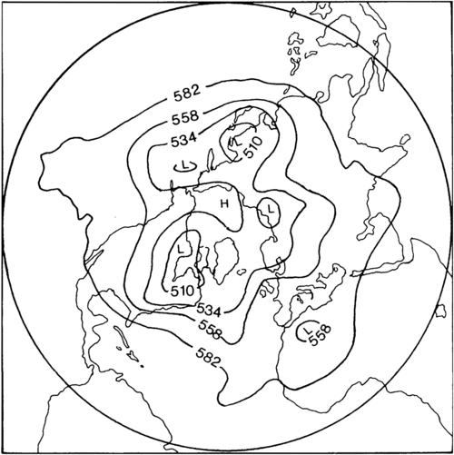
Figure 13.28 Observed height (in decameters = km/100) of the 50 kPa (500 mb) pressure surface in the northern hemisphere. The North Pole lies at the center of the picture. The undulations are due to Rossby waves. J. T. Houghton, The Physics of the Atmosphere, 1986; reprinted with the permission of Cambridge University Press.

Quasi-Geostrophic Vorticity Equation

The first step is to derive the governing equation for quasi-geostrophic motions using the customary β-plane approximation valid for βy ≪ f₀, keeping in mind that the approximation is not an especially good one for atmospheric Rossby waves, which have planetary scales. Although Rossby waves are frequently superposed on a mean flow, the equations are derived here without a mean flow. Instead, a uniform mean flow is added at the end, assuming that the perturbations are small and that a linear superposition is valid. The first step is to simplify the vorticity equation for quasi-geostrophic motions, assuming that the velocity is geostrophic to the lowest order. The small departures from geostrophy, however, are important because they determine the evolution of the flow with time.

Start with the shallow-water potential vorticity equation (13.94), and rewrite it as:

hDDt(ζ+f)−(ζ+f)DhDt=0.

Expand the material derivatives and substitute h = H + η, where H is the uniform undisturbed depth of the layer, and η is the surface displacement. This gives:

(H+η)(∂ζ∂t+u∂ζ∂x+v∂ζ∂y+βv)−(ζ+f0)(∂η∂t+u∂η∂x+v∂η∂y)=0.

(13.114)

where Df/Dt = v(df/dy) = βv has been used, and f has been replaced by f₀ in the second term because the usual β-plane approximation neglects the variation of f except for terms involving df/dy. For small perturbations, neglect the quadratic nonlinear terms in (13.114) to obtain:

H∂ζ∂t+Hβv−f0∂η∂t=0.

(13.115)

This is the linearized form of the potential vorticity equation. Its quasi-geostrophic version is obtained by inserting the approximate geostrophic expressions for velocity components:

u≅−gf0∂η∂y,andv≅gf0∂η∂x.

(13.116)

From these the vertical vorticity is found as:

ζ=∂v∂x−∂u∂y=gf0(∂2η∂x2+∂2η∂y2),

so that the linearized potential vorticity equation (13.115) becomes:

gHf0∂∂t(∂2η∂x2+∂2η∂y2)+gHβf0∂η∂x−f0∂η∂t=0.

(13.116)

Denoting c² = gH, this equation becomes:

∂∂t(∂2η∂x2+∂2η∂y2−f02c2η)+β∂η∂x=0,

(13.117)

which is the quasi-geostrophic form of the linearized vorticity equation for flow fields that span a significant range of latitude. The ratio c/f₀ is recognized as the Rossby radius. Note that ∂η/∂t was not set to zero in (13.115) to reach (13.117), although a strict validity of the geostrophic relations (13.116) would require that the horizontal divergence, and hence ∂η/∂t, be zero. This is because the departure from strict geostrophy determines the evolution of the flows described by (13.117). The geostrophic relations for the velocity can be used everywhere except in the horizontal divergence term in the vorticity equation.

Dispersion Relation

As for the prior wave motions considered in this chapter, assume the solutions of (13.117) will be in the form η=ηˆexp{i(kx+ly−ωt)}, and regard ω as positive; the signs of k and l then determine the direction of phase propagation. Substituting this assumed solution form into (13.117) gives:

ω=−βkk2+l2+f02/c2.

(13.118)

This is the dispersion relation for Rossby waves. The asymmetry of the dispersion relation with respect to k and l signifies that the wave motion is not isotropic in the horizontal, as is expected because of the β-effect. Although (13.118) was derived for a single homogeneous layer, it is equally applicable to stratified flows if c is replaced by the corresponding internal value, which is c² = g′H for the reduced-gravity model (see Section 8.7) and c = NH/nπ for the nth mode of a continuously stratified model. For the barotropic mode c is very large, so f02/c2 is usually negligible compared to other terms in the denominator of (13.118).

Using (13.118), ω(k,l) and can be displayed as a surface, taking k and l along Cartesian axes and plotting contours of constant ω. The section of this surface along l = 0 is indicated in the upper panel of Figure 13.29, and contours of the surface for three values of ω are indicated in the bottom panel. These contours are circles because (13.118) can be written as:

(k+β2ω)2+l2=(β2ω)2−f02c2.

In the lower panel of Figure 13.29, the arrows perpendicular to the constant-ω contours indicate directions of group velocity vector c_g:

cg=excgx+eycgy=ex∂ω∂k+ey∂ω∂l,

which is the gradient of ω in the wave number space. The direction of c_g is therefore perpendicular to the ω contours. For l = 0, the maximum frequency and zero group speed are attained at kc/f₀ = −1, corresponding to ω_max f₀/βc = 0.5. The maximum frequency is much smaller than the Coriolis frequency. For example, in the ocean the ratio ωmax/f0=0.5βc/f02 is of order 0.1 for the barotropic mode, and of order 0.001 for a baroclinic mode, taking a typical mid-latitude value of f₀ ∼ 10^–4 s⁻¹, a barotropic gravity wave speed of c ∼ 200 m/s, and a baroclinic gravity wave speed of c ∼ 2 m/s. The shortest period of mid-latitude baroclinic Rossby waves in the ocean can therefore be more than a year.

The eastward phase speed is:

cx=ωk=−βk2+l2+f02/c2.

(13.119)

The negative sign shows that the phase propagation is always westward. The phase speed reaches a maximum when k² + l² → 0, corresponding to very large wavelengths represented by the region near the origin of Figure 13.29. In this region the waves are nearly non-dispersive and have an eastward phase speed cx≅−βc2/f02. With β = 2 × 10⁻¹¹ m⁻¹ s⁻¹, a typical baroclinic value of c ∼ 2 m/s, and a mid-latitude value of f₀ ∼ 10⁻⁴ s⁻¹, this gives c_x ∼ 10⁻² m/s. At these slow speeds the Rossby waves would take years to cross the width of the ocean at mid-latitudes. Rossby waves in the ocean are therefore more important at lower latitudes, where they propagate faster. However, the dispersion relation (13.118), is not valid within a latitude band of 3° from the equator for which the assumption of a near geostrophic balance breaks down. A different analysis is needed in the tropics. A discussion of the wave dynamics of the tropics is given in Gill (1982) and in the review paper by McCreary (1985). In the atmosphere c is much larger, and consequently the Rossby waves propagate faster. A typical large atmospheric disturbance can propagate as a Rossby wave at a speed of several meters per second.

Figure 13.29 Dispersion relation ω(k,l) for a Rossby wave. The upper panel shows ω versus k for l = 0. Regions of positive and negative group velocity c_gx are indicated. The lower panel shows a plane view of the surface ω(k,l), showing contours of constant ω on a kl-plane. The values of ωf₀/βc for the three circles are 0.2, 0.3, and 0.4. Arrows perpendicular to the largest circular constant-ω contour indicate directions of the group velocity vector c_g. A. E. Gill, Atmosphere−Ocean Dynamics, 1982; reprinted with the permission of Academic Press and Mrs. Helen Saunders-Gill.

Frequently, Rossby waves are superposed on a strong eastward mean current, such as the atmospheric jet stream. If U is the speed of this eastward current, then the observed eastward phase speed is:

cx=U−βk2+l2+f02/c2.

(13.120)

Stationary Rossby waves can therefore form when the eastward current cancels the westward phase speed, giving c_x = 0. This is how stationary waves are formed downstream of the topographic step in Figure 13.20. A simple expression for the wavelength results if we assume l = 0 and the flow is barotropic, so that f02/c2 is negligible in (13.120). This gives U = β/k² for stationary Rossby waves, so that the wavelength is 2π[U/β]^1/2.

Finally, the derivation of the quasi-geostrophic vorticity equation provided in this section has not been rigorously justified in the sense that approximations have been made without a formal ordering of the scales. Gill (1982) provides a more rigorous derivation, expanding in terms of a small parameter. Another way to justify the dispersion relation (13.118) is to obtain it from the general dispersion relation (13.76). For ω ≪ f, the first term in (13.76) is negligible compared to the third, and when this term is dropped (13.76) reduces to (13.118).

Example 13.13

If the west coast of North America experiences relatively clear and dry winter weather (a ridge in the 500 mb isobar height) while the center of the continent 3,000 km to the east experiences relatively cool and cloudy conditions (a depression in the 500 mb isobar height), estimate the average eastward convection speed U of the atmosphere assuming these weather phenomena result from a stationary barotropic Rossby wave.

Solution

For an estimate, use the simplified version of (13.120), U = β/k² = βλ²/(2π)², and recognize that 3,000 km represents the peak-to-valley distance or half of the Rossby wavelength. The numerical values then imply:

U=βλ2(2π)2≅(2×10−11m−1s−1)(2·3×106m)24π2=18ms−1,

 

where a mid-latitude value of β = 2 × 10⁻¹¹ m⁻¹ s⁻¹, has been used. Although this speed is lower than values typically associated with the polar jet stream (30 to 50 m/s) in the northern hemisphere, it is in the right range given that it should represent a latitude- and altitude-averaged atmospheric convection speed.