2.1 Time Delay Model
Most of the nature of time delays has not been completely defined, therefore, it is a possibility to define these as uncertainties for several applications. Since there is not a unique nature of time delays, novel approaches become an affordable and competitive issue on course.
 ), and from controller node to actuator node (
 ).
).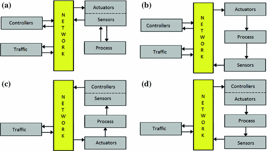
NCS common configurations
If the sensor and actuator nodes are the same as case A or all the nodes are completely distributed as case B, the controller node normally is able to measure the  , and estimate
  . In case C, if the sensor and controller nodes are the same,
  , and
, and  is estimated. Finally, the case D if the controller and actuator nodes are the same, the RTT is simply computed since
  can be directly measured and
  .
.
From previous configurations, the first two cases present both time delays  and
and  , and thus, the case B is the one to be used to apply the methodologies proposed in this book. As stated before, only this configuration allows to measure
  , but it is necessary to estimate
  .
.
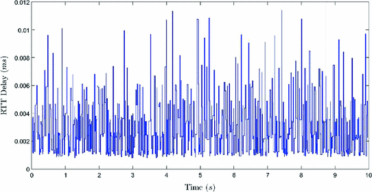
RTT delay measured from an Ethernet network at UNAM
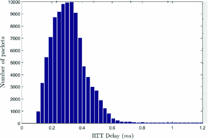
Histogram of RTT delays measured into an Ethernet network at UNAM

 is a location parameter defining by the median of the time delay and
  is a scale parameter defining by the standard deviation. The sample space is defined by the minimum RTT delay and the maximum allowable time delay bound (MATI) [3].
This distribution is computed for a time window with w previous measurements of time delay ( ), where a expected time delay value for RTT is
 ![$$E[\tau _{k|w}] = \varphi + \eta $$](../images/321711_1_En_2_Chapter/321711_1_En_2_Chapter_TeX_IEq16.png) with variance
with variance ![$$Var[\tau _{k|w}]=\varphi ^2$$](../images/321711_1_En_2_Chapter/321711_1_En_2_Chapter_TeX_IEq17.png) [4].
[4].
 . The median of the window is a feasible election, since it represents an expected time delay within the window. The distribution is obtained for each one of the values in the time window (
 ).
). ![$$P[\tau _k = \hat{\eta }_{k+1|w}]$$](../images/321711_1_En_2_Chapter/321711_1_En_2_Chapter_TeX_IEq20.png) represents the time delay with the maximum probability. Using this value, the expected time delay values of the median
represents the time delay with the maximum probability. Using this value, the expected time delay values of the median  and standard deviation
  are computed, and hence:
![$$\begin{aligned} \hat{\eta } _{k + 1|w} = w_i |P_{\mathop {\max }\limits _i } \left[ w \right] \end{aligned}$$](../images/321711_1_En_2_Chapter/321711_1_En_2_Chapter_TeX_Equ2.png)


2.2 Adaptive Fuzzy Model
The strategies for control systems with static time delays is common in literature. Nevertheless, strategies considering variable time delays are uncommon. Among this kind of strategies, it is used optimal control (LQR, LQG) [5, 6], robust control ( ) [7, 8], vanishing perturbation [9], and others. These strategies aim to keep a control input resilient to variations of time delays, no matter whether this is an optimal input for the NCS.
In this section, an proposed method is introduced using a fuzzy controller, its advantage is to generate optimal control signals for each time delay value. While, it is robust to variations in such time delays. First, the time delays are analyzed an modeled as Sect. 2.1.

 is the ith state, n is the number of states, r is the number of fuzzy rules, and
  is the related membership function. Thus:


 are the system states (fuzzy inputs), n is the number of states,
  are the system inputs, m is the number of system inputs,
  are the system outputs, q is the number of system outputs. Also,
  ,
,  , and
, and  are the plant representation per scenario according to current time delays, where n is the number of states, m is the number of inputs of the system, and r is the number of fuzzy rules, as shown in Fig. 2.4.
 for the plant. The Eq. 2.9 models some kinds of faults using a vector
  . So,
. So,  masks the plant faults and the model (2.9) is considering a local variable structure when faults occur and incorporating the time delays
  and
and  . Remember, the nature of fault is out of the scope of this book. Notice that
  is the relation of a fault presence through the event.
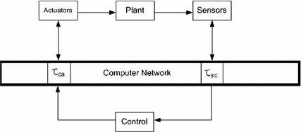
Organization of nodes for a NCS

![$$[t_i, t_{i+1}]$$](../images/321711_1_En_2_Chapter/321711_1_En_2_Chapter_TeX_IEq38.png) is:
is:
 is the input matrix and
  is the state matrix of the continuous model of the plant. Remember that
  is the total number of local time delays that appears per scenario, and they respectively are the source of
  and
and  . Suppose that the system is in a stable equilibrium point. Thus, the only perturbations are the time delays, and hence, it is possible to assume the outputs
  of the plant.

 is the feedback state for control.
Since the observed states need to be guaranteed, it is necessary to define a group of observers. The proposal of a control law in Sect. 4.2 use a group of observers to guarantee as well the system structure and the local time delays are integrated into the dynamic structure. Therefore, stability, in terms of time delays and misleading structure, should be accomplished. A review of the control law is developed through the following chapters. The related observer states are presented as z(k). In this case  and
and  are the observer parameters, to be defined in Sect. 4.2 [11].
2.3 Sampling Frequency Model
One of the strategies implemented for NCS control is feedback scheduling, where the goal is to know the performance of the communication network to modify the transmission of each node and improve the performance of the whole system.
The proposal for feedback scheduling into a real-time distributed system modifies the transmission frequency of each node into a region where the performance in each node is acceptable. This approach is a representation of the transmission frequencies using a time-invariant space state system, whose state variables are the desired transmission frequencies  with
with  of the n nodes involved in the NCS.
 and maximum
  transmission frequency computed offline. The
  are defined by the steady-state stability requirements associated to the node i and the
  are defined by the capacity of the node i itself without generating an excessive transmission cost into the network i.e. in a distributed system with n nodes, each one performing a task
  with a maximum frequency
  and consumption time per transmission packet
  , for
, for  the following computational constraint needs to be accomplished:
So, the state variables  are the desired frequencies of the n nodes in the network control system. The objective of the proposed controller is to stabilize the current frequency of the system
  to the desired reference frequency
  , through an optimal trajectory using a LQR controller.
![$$\begin{aligned} x[k + 1]= & {} Ax[k] + Bu[k] \\ y[k]= & {} Cx[k] \nonumber \end{aligned}$$](../images/321711_1_En_2_Chapter/321711_1_En_2_Chapter_TeX_Equ14.png)
 is the matrix of relationships between frequencies of the nodes,
  is the weighted frequency matrix,
  is the output matrix,
  is a real frequency vector, and
  is the next frequency vector.
 be given by a function of minimal frequencies
  and
and  given by a function of maximal frequencies
  , where
  ,
,  and n nodes:

 and
and  in Eq. 2.14 are defined as follows:


2.4 Control-Scheduling Codesign Model

 is the output matrix, and matrices
  y
y  are obtained using:
 and
and  as the matrices of the system and input of the model in continuous form:
 , with
  , is [12]:
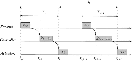
Execution time of control tasks with instants of actuation
![$$x(s,k) \in [t(k-1),t(k)]$$](../images/321711_1_En_2_Chapter/321711_1_En_2_Chapter_TeX_IEq81.png) are obtained, and the instants of actuation are labelled by t(k) where the control signals u(k) are applied. Hence, the time elapsed between consecutive instants of actuation
are obtained, and the instants of actuation are labelled by t(k) where the control signals u(k) are applied. Hence, the time elapsed between consecutive instants of actuation ![$$[t(k-1),t(k)]$$](../images/321711_1_En_2_Chapter/321711_1_En_2_Chapter_TeX_IEq82.png) , has a actuating period h. The difference between the sampling instant t(s, k) and the following actuation instant t(k) is a variable time delay:
, has a actuating period h. The difference between the sampling instant t(s, k) and the following actuation instant t(k) is a variable time delay:

 in Eq. 2.24 can vary at each closed-loop operation. The interested reader is referred to [14] for further reading on this control model.
Each instant of actuation, the actuator node generates the next actuation instant t(k), which is sent to the sensor after applying the control signal  to the plant. Upon reception of this message or next sampling period, the sensor samples the plant x(s, k), and records the absolute sampling time t(s, k). The latter, together with t(k), is used to compute
  . Both x(s, k) and
  are sent to the controller node. Upon reception of this message, the controller node estimates the plant state that applies at
  (Eq. 2.25) with the next estimated time delay
  , and computes a control command u(k) designed in Chap. 4. This is sent to the actuator that applies it to the plant at the synchronised actuation instant.
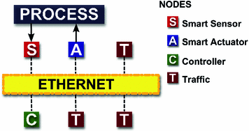
NCS configuration
All nodes send User Datagram Protocol (UDP) packets to avoid double traffic into network. However, it is not possible to know whether there is packets loss or a maximum time delay since there is no acknowledgement that the sent packet has been received.
Here, network-induced time delays and variable sampling intervals smaller than a sampling period are compensated by the one-shot model, and the fuzzy model compensates time delays longer than such a sampling period.
 . Once the time delay
  is received, an exponential distribution algorithm [15] is used to estimate the next time delay
  . This algorithm is widely used to estimate delays in real time, where an offline statistical analysis characterises mean and standard deviation
  of time delays data
  with multiple scenarios of traffic. Those are used to form a generalized exponential distribution with a probability density function (Eq. 2.1).
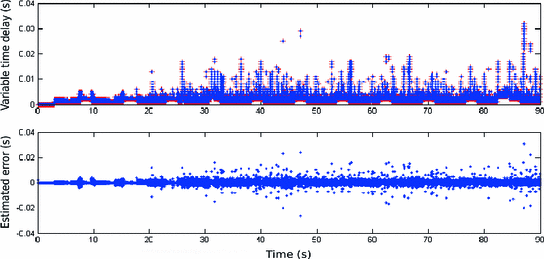
Variable time delay ( ) behaviour and estimation error with algorithm in Sect. 2.1
Once the next time delay  of the system is estimated, it is used to generate a control signal. This controller starts with a fuzzy model of the NCS, designed as follows.
 as input of the antecedent part, and linear discrete models with different sampling periods
  as consequent part. Thus, defining r fuzzy rules, the jth rule has the form:
 is the state vector of system,
  is the input vector of process,
  is the jth membership function of the estimated time delay
  .
.
 is:
is:
 is a Gaussian membership function with parameters
  .
.  are the matrices of jth linear discrete model discretised with a sampling period
  (
( ). The discrete local models are:
 for
for  are assigned by user according to offline time delay measurement.
With this fuzzy model, the estimated state of a system is obtained by compensating the time delays and variable sampling intervals. The action is to smoothly switch between discrete models, to generate the best estimate of state, according to the estimated time delay  . Once designed the fuzzy model (2.26) using the estimated time delay
  , a fuzzy controller is proposed in Chap. 4.
2.5 Neuro-Fuzzy Identification
The objective of the neuro-fuzzy model is to define the best linear model for each sampling period representing the system. This model estimates the system states according to the possible time delay calculated by an exponential distribution function defined in Sect. 2.1.
 as antecedent input, and discrete models with different sampling periods T as consequent part. So, defining r fuzzy rules, the jth rule has the form:
 is the state vector of the system,
  is the input vector of the plant,
  is the jth membership function of variable sampling period
  .
.
 is:
is:
 is a Gaussian membership function with parameters
  , and
, and  and
and  are the matrices of jth linear model, with m outputs and periods
  .
.The system states are approximated with this fuzzy model. The objective is to smoothly switch between discrete models, to generate the best estimate of states according to the variable sampling period . However, there are some parameters such as
  that need to be tuned using a neuro-fuzzy approach [18, 19]. This section uses data of the simulated system with some specific time delays to get the model parameters, although, alternatively techniques like LMI may be used and reviewed in other works as [20]. The neuro-fuzzy model (Eq. 2.30) is identified using inputs-states data with measured variable sampling period
  , obtained from a Truetime simulation of the system [21], with a PID controller and a traffic node on an Ethernet network.
The identification procedure has two algorithms: a clustering algorithm, to create new rules, and a training algorithm, to update the model’s parameters. The procedure is repeated  -epochs. M is maximum firing strength of all rules for variable sampling period and
  is its threshold.
  is a threshold of maximum model error. J is the performance index to update the matrices
  .
.
 , which is the variable sampling period mean, and
  is the predetermined width. So, matrices
  and
and  of the first rule are:


 -completeness criterion, which states that, for any input within operation range, there is a rule with fire strength
  greater than a threshold
  [22]. So, if maximum firing strength M of all rules is less than
  then a new rule is created.

 (Eq. 2.40), the parameters should be adjusted. The threshold
  is decreased according to the current epoch f.


 is the final error expected at the end of training,
  is the initial error obtained in the first epoch without training, f is the current training epoch, and
  is the total of epochs.
 and
and  of the system
  and control
  matrices, respectively, as well as the centres and standard deviations are adjusted by:


 is the learning rate for each parameter,
  ,
,  ; and
; and  . The data used in here is the result of analysis of general scenarios considering local time delays and ethernet channel communication.
Once designed and identified, the fuzzy model (Eqs. 2.30, 2.31, 2.32) is presented a fuzzy controller in Chap. 4, using estimated variable sampling period  .
.
2.6 Concluding Remarks
This chapter presents a statistical model of the time delay through an exponential probability density function that allows estimating the time delay for compensation purposes, the model assumes a variable time delay and greater than the sampling period of the system, Model is validated using experimental data. Three design methodologies are also presented.
The first method presents a model using fuzzy theory to incorporate the estimated time delay with several space-state models. This allows improving the state estimation to be used in the controller with minimal computational cost.
The second method presents a sampling frequency model through a state-space model that represents the dynamic behaviour of the transmission frequency as a function of the actual transmission frequency into the network with longer time delays or lost deadlines.
The third method presents a methodology of codesign where through two fuzzy models are trade-off the control and scheduling performance. The first model incorporates linear models with different sampling periods obtaining delay-dependent system states. The second model uses QsC and QsS to schedule the next stable actuation period and minimise the system error and the effect of network uncertainties.
Finally, a neural strategy is presented to obtain the fuzzy rules that allow to identify the complete NCS system and to improve the estimation of the states of the system.