CHAPTER 6
Demand, Supply, Market Equilibrium, and Welfare Analysis
IN THIS CHAPTER
Summary: A thorough understanding of the way in which the market system determines price and quantity pays dividends both in microeconomics and macroeconomics. In the absence of government intervention and/or externalities, the competitive market also provides the most efficient outcome for society.

Key Ideas
 Demand
 Supply
 Equilibrium
 Consumer and Producer Surplus
6.1 Demand
Main Topics: Law of Demand, Income and Substitution Effects, The Demand Curve, Quantity Demanded Versus Demand, Determinants of Demand
For many years now, you have understood the concept of demand. On the surface, the concept is rather simple: people tend to purchase fewer items when the price is high than they do when the price is low. This is such an intuitively appealing concept that your typical consumer cares little about the rationale and still manages to live a happy life. As someone knee-deep in reviewing to take the AP Microeconomics Exam, you need to go “behind the scenes” of demand. Intuition will take you only so far; you need to know the underlying theory of what is perhaps the most widely understood, and sometimes misunderstood, economic concept.
Law of Demand

Let’s get this part out of the way. The law of demand is commonly described as: Holding all else equal (ceteris paribus), when the price of a good rises, consumers decrease their quantity demanded for that good. In other words, there is an inverse, or negative, relationship between the price and the quantity demanded of a good.
“Holding all else equal”? Economic models—demand is just one of many such models—are simplified versions of real behavior. In addition to the price, there are many factors that influence how many units of a good consumers purchase. In order to predict how consumers respond to changes in one variable (price), we must assume that all other relevant factors are held constant. Say we observed that last month the price of orange juice fell, consumer incomes rose, the price of apple juice increased, and consumers bought more orange juice. Was this increased orange juice consumption because the price fell, because incomes rose, or perhaps because apple juice became more expensive? Maybe it increased for all of these reasons. Maybe for none of these reasons. It is impossible to isolate and measure the effect of one variable (i.e., orange juice prices) on the consumption of orange juice if we do not control (hold constant) these other external factors. At the heart of the law of demand is a consumer’s willingness and ability to pay the going price. If the consumer becomes more willing, or more able, to consume a good, then either the price has fallen or one of these external factors has changed. We spend more time on these demand “determinants” a little later in this chapter.
Income and Substitution Effects
One of the important factors behind the scenes of the law of demand is the economic mantra “only relative prices matter.” I’m sure you have heard the stories from your parents or grandparents about how the price of a cup of coffee back in the good old days was just a nickel. Today you might get the same coffee for $1.75. These prices are simply money (or absolute, or nominal) prices, and when it comes to a demand decision, a money price alone is near useless. However, if you think about the money price in terms of (1) what other goods $1.75 could buy, or (2) how much of your income is absorbed by $1.75, then you’re talking relative (or real) prices. These are what matter. The number of units of any other good Y that must be sacrificed to acquire the first good X, measures the relative price of good X.
Example:
Let’s keep things simple and say that you divide your $10 daily income between apple fritters at today’s prices of $1 each and chocolate chip bagels at $2 each. These are the money prices of your labor and of these two yummy snacks.
Today at the price of $1, the relative cost of a fritter is one-half of a bagel (see Table 6.1). Relative to your income, it amounts to one-tenth of your budget.
Table 6.1

Tomorrow, when the price doubles to $2 per fritter, two things happen to help explain, and lay the foundation for, the law of demand:
1. The relative price of a fritter has risen to one bagel, and the relative price of a bagel has fallen from two fritters to one fritter. Since fritters are now relatively more expensive, we would expect you to consume more bagels and fewer fritters. This is known as the substitution effect.
2. Relative to your income, the price of a fritter has increased from one-tenth to one-fifth of your budget. In other words, if you were to buy only fritters, today you can purchase 10 but tomorrow the same income would only buy you 5. This lost purchasing power is known as the income effect.

• Substitution effect. The change in quantity demanded resulting from a change in the price of one good relative to the price of other goods.
• Income effect. The change in quantity demanded resulting from a change in the consumer’s purchasing power (or real income).
When the price of fritters increased, both of these effects caused our consumer (you) to decrease the quantity demanded, thus predicting a response consistent with the law of demand.
So at this point you might ask, “How would a consumer react if the prices of fritters and bagels and daily income had all doubled?”
Since the price of fritters, relative to the price of bagels, and relative to daily income, has not changed, the consumer is unlikely to alter behavior. This is why we say that only relative prices matter.
The Demand Curve
The residents of a small Midwestern town love to quench their summer thirsts with lemonade. Table 6.2 summarizes the townsfolk’s daily consumption of cups of lemonade at several prices, holding constant all other factors that might influence the overall demand for lemonade. This table is sometimes referred to as a demand schedule.
Table 6.2
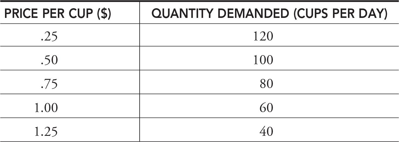
The values in Table 6.2 reflect the law of demand: Holding all else equal, when the price of a cup of lemonade rises, consumers decrease their quantity demanded for lemonade. It is often quite useful to convert a demand schedule like the one above into a graphical representation, the demand curve (Figure 6.1).
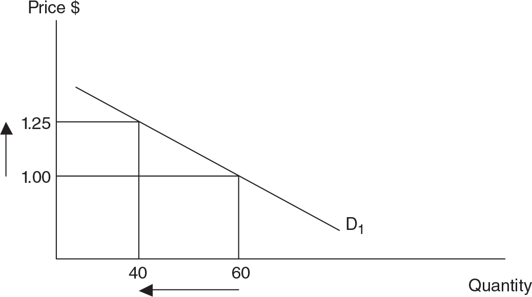
Figure 6.1
Quantity Demanded Versus Demand

The law of demand predicts a downward- (or negative-) sloping demand curve (Figure 6.1). If the price moves from $1 to $1.25 and all other factors are held constant, we observe a decrease in the quantity demanded from 60 to 40 cups. It is important to place special emphasis on “quantity demanded.” If the price of the good changes and all other factors remain constant, the demand curve is held constant and we simply observe the consumer moving along the fixed demand curve. If one of the external factors change, the entire demand curve shifts to the left or right.
Determinants of Demand

So, what are all of these factors that we insist on holding constant? These determinants of demand influence both the willingness and ability of the consumer to purchase units of the good or service. In addition to the price of the product itself, there are a number of variables that account for the total demand of a good like lemonade:
• Consumer income.
• The price of a substitute good such as iced tea.
• The price of a complementary good such as a Popsicle.
• Consumer tastes and preferences for lemonade.
• Consumer expectations about future prices of lemonade.
• Number of buyers in the market for lemonade.
• Consumer Income
Demand represents the consumer’s willingness and ability to pay for a good. Income is a major factor in that “ability” to pay component. For most goods, when income increases, demand for the good increases. Thus, for these normal goods, increased income results in a graphical rightward shift in the entire demand curve. There are other inferior goods, fewer in number, where higher levels of income produce a decrease in the demand curve.
Example:
When looking to furnish a first college apartment, many students increase their demand for used furniture at yard sales. Upon graduation and employment in their first real job, new graduates increase their demand for new furniture and decrease their demand for used furniture. For them, new furniture is a normal good, while used furniture is an inferior good.

• An increase in demand is viewed as a rightward shift in the demand curve. There are two ways to think about this shift.
a. At all prices, the consumer is willing and able to buy more units of the good. In Figure 6.2 you can see that at the constant price of $1, the quantity demanded has risen from two to three.
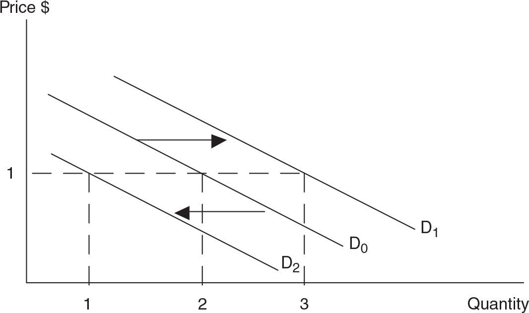
Figure 6.2
b. At all quantities, the consumer is willing and able to pay higher prices for the good.
• Of course, the opposite is true of a decrease in demand, or leftward shift of the demand curve. In Figure 6.2 you can see that at the constant price of $1, the quantity demanded has fallen from two to one.
• Price of Substitute Goods
Two goods are substitutes if the consumer can use either one to satisfy the same essential function, therefore experiencing the same degree of happiness (utility). If the two goods are substitutes, and the price of one good X falls, the consumer demand for the substitute good Y decreases.
Example:
Mammoth State University (MSU) and Ivy Vine College (IVC) are considered substitute institutions of higher learning in the same geographical region. Ivy Vine College, shamelessly seeking to increase its reputation as an “elite” institution, increases tuition, while Mammoth State’s tuition remains the same. We expect to see, holding all else constant, a decrease in quantity demanded for IVC degrees, and an increase in the overall demand for MSU degrees. (See Figures 6.3 and 6.4.)
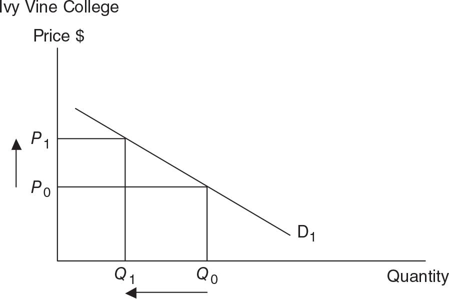
Figure 6.3
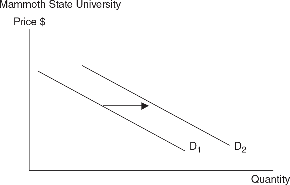
Figure 6.4
• Price of Complementary Goods
Two goods are complements if the consumer receives more utility from consuming them together than she would receive consuming each separately. I enjoy consuming tortilla chips by themselves, but my utility increases if I combine those chips with a complementary good like salsa or nacho cheese dip. If any two goods are complements, and the price of one good X falls, the consumer demand for the complement good Y increases.
“Finally, something in a textbook that I can fathom!”
—Adam, AP Student
Example:
College students love to order late-night pizza delivered to their dorm rooms. The local pizza joint decreased the price of breadsticks, a complement to the pizzas. We expect to see, holding all else constant, an increase in quantity demanded for breadsticks, and an increase in the demand for pizzas.
• Tastes and Preferences
We have different internal tastes and preferences. Collectively, consumer tastes and preferences change with the seasons (more gloves in December, fewer lawn chairs); with fashion trends; or with advertising. A stronger preference for a good is an increase in the willingness to pay for the good, which increases demand.
• Future Expectations
The future expectation of a price change or an income change can cause demand to shift today. Demand can also respond to an expectation of the future availability of a good.
Example:
On a Wednesday, you have reason to believe that the price of gasoline is going to rise $.05 per gallon by the weekend. What do you do? Many consumers, armed with this expectation, increase their demand for gasoline today. We might predict the opposite behavior, a decrease in demand today, if consumers expect the price of gasoline to fall a few days from now.
Demand can also be influenced by future expectations of an income change.
Example:
One month prior to your college graduation day, you land your first full-time job. You have signed an employment contract that guarantees a specific salary, but you will not receive your first paycheck until the end of your first month on the job. This future expectation of a sizable increase in income often prompts consumers to increase their demand for normal goods now. Maybe you would start shopping for a car, a larger apartment, or several business suits.
Example:
For years, auto producers have been promising more alternative-fuel cars, but so far these cars are relatively difficult to find on dealership lots. Suppose the “Big 3” promise widespread availability of affordable electric and hydrogen fuel cell cars in the next 12 months. This expectation of increased availability in the future will likely decrease the demand for these cars today.
• Number of Buyers
An increase in the number of buyers, holding other factors constant, increases the demand for a good. This is often the result of demographic changes or increased availability in more markets.
Example:
When the Soviet Union fractured and the Russian government began allowing more foreign investment, corporations such as Coca-Cola, Apple, and McDonald’s found millions of new buyers for their products. Globally, the demand for colas, iPads, and burgers increased.
Example
As the average age of Americans has gradually increased, there are now more people above the age of 70 years old. This demographic change has caused an increase in the demand for prescription drugs, hip replacements, and other medical services.
6.2 Supply
Main Topics: Law of Supply, Increasing Marginal Costs, The Supply Curve, Quantity Supplied Versus Supply, Determinants of Supply
If there are three words that you need to have in your arsenal for the AP exams, they are “Demand and Supply,” or “Supply and Demand” if you are the rebellious type. The previous section covered the demand half of this duo, and so it stands to reason that we should spend a little time studying the other side. Unlike demand, few of us have ever had up-close-and-personal experience as suppliers. Because you likely lack such personal experience with supply, it is helpful to put yourself in the shoes of someone who wishes to profit from the production and sale of a product. If something happens that would increase your chances of earning more profit, you increase your supply of the product. If something happens that will hurt your profit opportunities, you decrease your supply of the product.

Law of Supply
Drumroll, please. The law of supply is commonly described as: “Holding all else equal (ceteris paribus), when the price of a good rises, suppliers increase their quantity supplied for that good.” In other words, there is a direct, or positive, relationship between the price and the quantity supplied of a good.
Again, we insist on qualifying our law with the phrase, “Holding all else equal.” Similar to the demand model, the supply model is a simplified version of real behavior. In addition to the price, there are several factors that influence how many units of a good producers supply. In order to predict how producers respond to fluctuations in one variable (price), we must assume that all other relevant factors are held constant. Before we talk about these external supply determinants, let’s examine what is happening behind the scenes of the law of supply.
Increasing Marginal Costs
The more you do something (e.g., a physical activity), the more difficult it becomes to do the next unit of that activity. Anyone who has run laps around a track, lifted weights, or raked leaves in the yard understands this. If you were asked to rake leaves, as more hours of raking are supplied, it becomes physically more and more difficult to rake the next hour. We also include the opportunity cost of the time involved in the raking, and you surely know that time is precious to a student. If you have a paper to write or an exam to cram for, raking leaves for an hour comes at a dear cost. In terms of forgone opportunities, the marginal cost of raking leaves rises as you postpone that paper or study session.
When we discussed production possibilities in Chapter 5, we addressed a key economic concept: as more of a good is produced, the greater is its marginal cost.

• As suppliers increase the quantity supplied of a good, they face rising marginal costs.
• As a result, they only increase the quantity supplied of that good if the price received is high enough to at least cover the higher marginal cost.
The Supply Curve
A small town has a thriving summer sidewalk lemonade stand industry. Table 6.3 summarizes the daily quantity of cups of lemonade offered for sale at several prices, holding constant all other factors that might influence the overall supply of lemonade. This table is sometimes referred to as a supply schedule.
Table 6.3
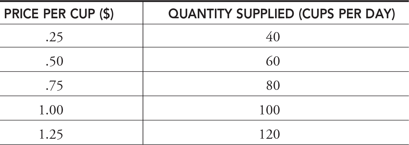
The values in this table reflect the law of supply: “Holding all else equal, when the price of a cup of lemonade rises, suppliers increase their quantity supplied for lemonade.” Remember those profit opportunities? If kids can sell more cups of lemonade at a higher price, they will do so. It is often quite useful to convert a supply schedule like the one in Table 6.3 into a graphical representation, the supply curve (Figure 6.5).
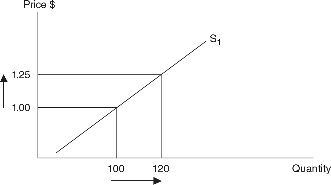
Figure 6.5
“Make sure on the AP test to include all labels, especially arrows.”
—Adam, AP Student
Quantity Supplied Versus Supply
“This is an important distinction to make.”
—AP Teacher
The law of supply predicts an upward- (or positive-) sloping supply curve (Figure 6.5). When the price moves from $1 to $1.25, and all other factors are held constant, we observe an increase in the quantity supplied from 100 cups to 120 cups. Just as with demand, it is important to place special emphasis on “quantity supplied.” When the price of the good changes, and all other factors are held constant, the supply curve is held constant; we simply observe the producer moving along the fixed supply curve. If one of the external factors changes, the entire supply curve shifts to the left or right.
Determinants of Supply
Lemonade producers are willing and able to supply more lemonade if something happens that promises to increase their profit opportunities. In addition to the price of the product itself, there are a number of variables, or determinants of supply, that account for the total supply of a good like lemonade:

• The cost of an input (e.g., sugar) to the production of lemonade
• Technology and productivity used to produce lemonade
• Taxes or subsidies on lemonade
• Producer expectations about future prices
• The price of other goods that could be produced
• The number of lemonade stands in the industry
• Cost of Inputs
If the cost of sugar, a key ingredient in lemonade, unexpectedly falls, it has now become less costly to produce lemonade, and so we should expect producers all over town, seeing the profit opportunity, to increase the supply of lemonade at all prices. This results in a graphical rightward shift in the entire supply curve.

• An increase in supply is viewed as a rightward shift in the supply curve. There are two ways to think about this shift:
1. At all prices, the producer is willing and able to supply more units of the good. In Figure 6.6 you can see that at the constant price of $1, the quantity supplied has risen from two to three.
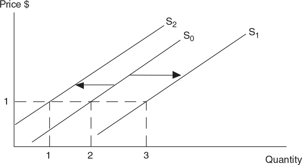
Figure 6.6
2. At all quantities, the marginal cost of production is lower, so producers are willing and able to accept lower prices for the good.
• Of course, the opposite is true of a decrease in supply, or leftward shift of the supply curve. In Figure 6.6 you can see that at the constant price of $1, the quantity supplied has fallen from two to one.
• Technology or Productivity
A technological improvement usually decreases the marginal cost of producing a good, thus allowing the producer to supply more units, and is reflected by a rightward shift in the supply curve. If kids all over town began using electric lemon squeezers rather than their sticky bare hands, the supply of lemonade would increase.
• Taxes and Subsidies
A per-unit tax is treated by the firm as an additional cost of production and would therefore decrease the supply curve, or shift it leftward. Mayor McScrooge might impose a 25-cent tax on every cup of lemonade, decreasing the entire supply curve. A subsidy is essentially the anti-tax, or a per-unit gift from the government because it lowers the per-unit cost of production.
“Remember, the tax goes to the government and is NOT included in the profit.”
—Hillary, AP Student
• Price Expectations
A producer’s willingness to supply today might be affected by an expectation of tomorrow’s price. If it were the 2nd of July and lemonade producers expected a heat wave and a 4th of July parade in two days, they might hold back some of their supply today and hope to sell it at an inflated price on the holiday. Thus, today’s quantity supplied at all prices would decrease.
• Price of Other Outputs
Firms can use the same resources to produce different goods. If the price of a milkshake were rising and profit opportunities were improving for milkshake producers, the supply of lemonade in a small town would decrease and the quantity of supplied milkshakes would increase.
• Number of Suppliers
When more suppliers enter a market, we expect the supply curve to shift to the right. If several of our lemonade entrepreneurs are forced by their parents to attend summer camp, we would expect the entire supply curve to move leftward. Fewer cups of lemonade would be supplied at each and every price.
6.3 Market Equilibrium
Main Topics: Equilibrium, Shortage, Surplus, Changes in Demand, Changes in Supply, Simultaneous Changes in Demand and Supply
Demanders and suppliers are both motivated by prices, but from opposite camps. The consumer is a big fan of low prices; the supplier applauds high prices. If a good were available, consumers would be willing to buy more of it, but only if the price is right. Suppliers would love to accommodate more consumption by increasing production, but only if justly compensated. Is there a price and a compatible quantity where both groups are content? Amazingly enough, the answer is a resounding “maybe.” Discouraged? Don’t be. For now we assume that the good is exchanged in a free and competitive market, and if this is the case, the answer is “yes.” We explore the “maybes” in a later chapter.
Equilibrium

The market is in a state of equilibrium when the quantity supplied equals the quantity demanded at a given price. Another way of thinking about equilibrium is that it occurs at the quantity where the price expected by consumers is equal to the price required by suppliers. So if suppliers and demanders are, for a given quantity, content with the price, the market is in a state of equilibrium. If there is pressure on the price to change, the market has not yet reached equilibrium. Let’s combine our lemonade tables from the earlier sections in Table 6.4.
Table 6.4
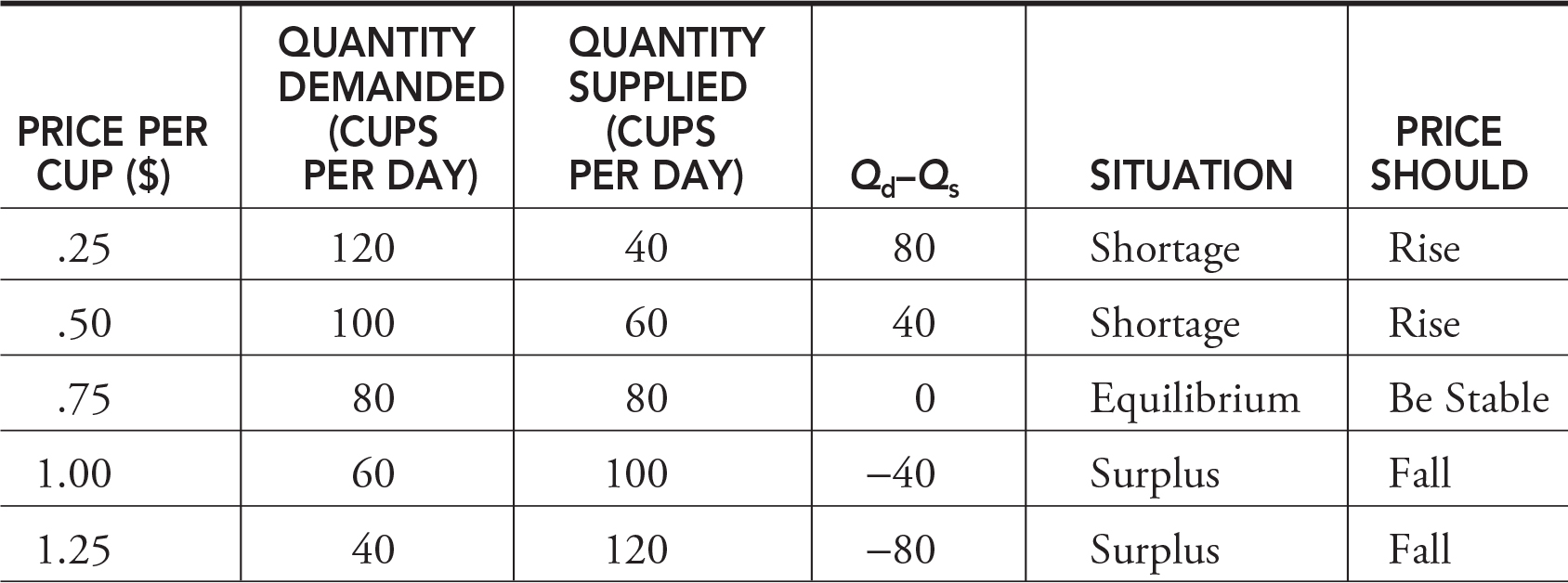
At a price of 75 cents, the daily quantity demanded and quantity supplied are both equal to 80 cups of lemonade. The equilibrium (or market clearing) price is therefore 75 cents per cup. In Figure 6.7 the equilibrium price and quantity are located where the demand curve intersects the supply curve. Holding all other demand and supply variables constant, there exists no other price where Qd = Qs.
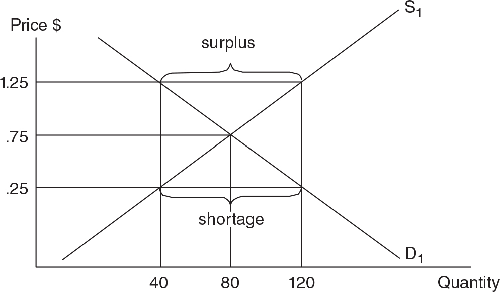
Figure 6.7
Shortage
“In a free market, shortages and surpluses always return to equilibrium in the long run.”
—Adam, AP Student
A shortage exists at a market price when the quantity demanded exceeds the quantity supplied. This is why a shortage is also known as excess demand. At prices of 25 cents and 50 cents per cup, you can see the shortage in Figure 6.7. Remember that consumers love low prices so the quantity demanded is going to be high. However, suppliers are not thrilled to see low prices and therefore decrease their quantity supplied. At prices below 75 cents per cup, lemonade buyers and sellers are in a state of disequilibrium. The disparity between what the buyers want at 50 cents per cup and what the suppliers want at that price should remedy itself. Thirsty demanders offer lemonade stand owners prices slightly higher than 50 cents, and, receiving higher prices, suppliers accommodate them by squeezing lemons. With competition, the shortage is eliminated at a price of 75 cents per cup.
Surplus
A surplus exists at a market price when the quantity supplied exceeds the quantity demanded. This is why a surplus is also known as excess supply. At prices of $1 and $1.25 per cup, you can see the surplus in Figure. 6.7. Consumers are reluctant to purchase as much lemonade as suppliers are willing to supply, and, once again, the market is in disequilibrium. To entice more consumers to buy lemonade, lemonade stand owners offer slightly discounted cups of lemonade and buyers respond by increasing their quantity demanded. Again, with competition, the surplus would be eliminated at a price of 75 cents per cup.
• Shortages and surpluses are relatively short-lived in a free market as prices rise or fall until the quantity demanded again equals the quantity supplied.

Changes in Demand
While our discussion of market equilibrium implies a certain kind of stability in both the price and quantity of a good, changing market forces disrupt equilibrium, either by shifting demand, shifting supply, or shifting both demand and supply.
“Explain your logic every time you shift a curve, no matter what!”
—Jake, AP Student
Increase in Demand
About once a winter a freak blizzard hits southern states like Georgia and the Carolinas. You can bet that the national media show video of panicked southerners scrambling for bags of rock salt and bottled water. Inevitably a bemused reporter tells us that the price of rock salt has skyrocketed to $17 per bag. What is happening here? In Figure 6.8, the market for rock salt is initially in equilibrium at a price of $2.79 per bag. With a forecast of a blizzard, consumers expect a lack of future availability for this good. This expectation results in a feverish increase in the demand for rock salt, and, at the original price of $2.79, there is a shortage. The market’s cure for a shortage is a higher equilibrium price. (Note: The equilibrium quantity of rock salt might not increase much, since blizzards are short-lived and the supply curve might be nearly vertical.)
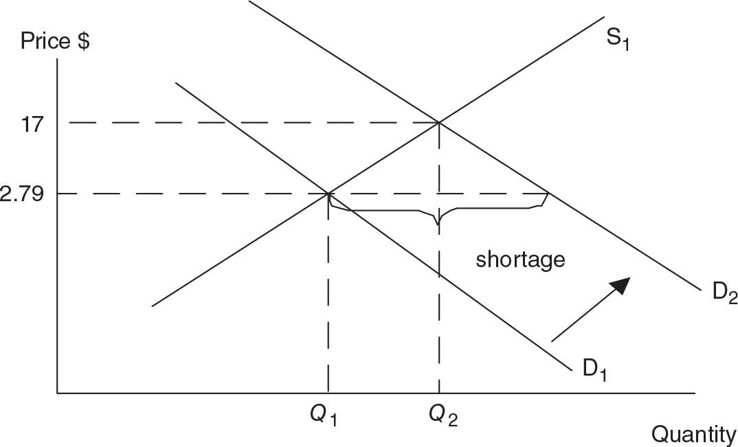
Figure 6.8
Decrease in Demand
The most recent recession was damaging to the automobile industry. When average household incomes fell in the United States, the demand for cars, a normal good, decreased. Manufacturers began offering deeply discounted sticker prices, zero-interest financing, and other incentives to reluctant consumers so that they might purchase a new car. In Figure 6.9 you can see that the original price of a new car was $18,000. Once the demand for new cars fell, there was a surplus of cars on dealer lots at the original price. The market cure for a surplus is a lower equilibrium price; therefore, fewer new cars were bought and sold.
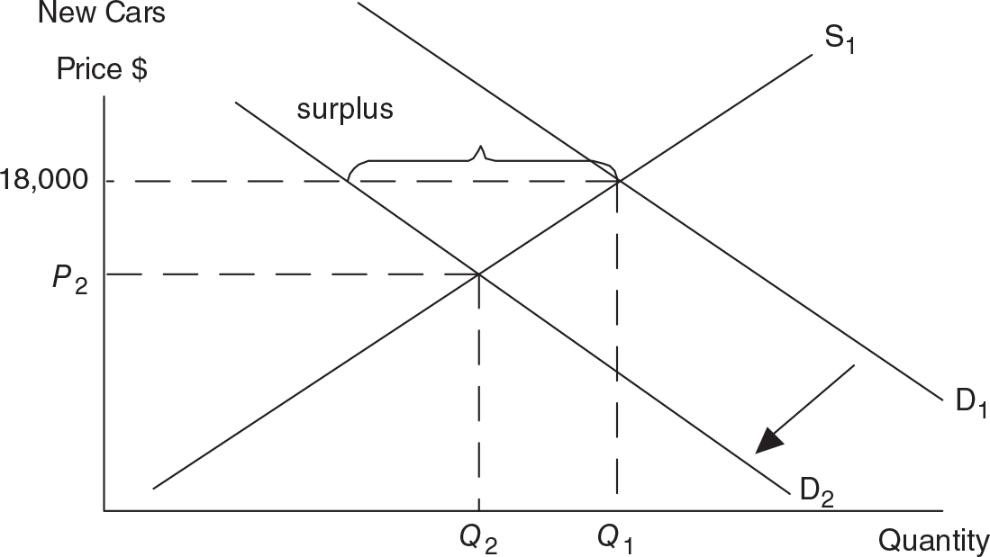
Figure 6.9

• When demand increases, equilibrium price and quantity both increase.
• When demand decreases, equilibrium price and quantity both decrease.
Changes in Supply
Increase in Supply
Advancements in computer technology and production methods have been felt in many markets. Figure 6.10 illustrates how, because of better technology, the supply of laptop computers has increased. At the original equilibrium price of $4,000, there is now a surplus of laptops. To eliminate the surplus, the market price must fall to P2 and the equilibrium quantity must rise to Q2.
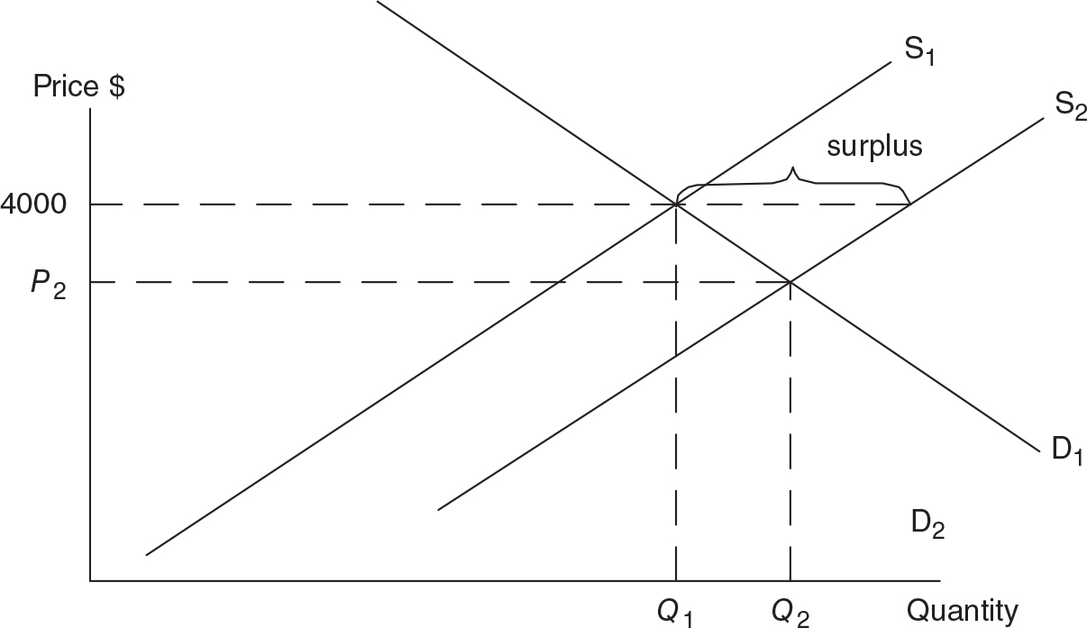
Figure 6.10
Decrease in Supply
Geopolitical conflict in the Middle East usually slows the production of crude oil. This decrease in the global supply of oil can be seen in Figure 6.11. At the original equilibrium price of $60 per barrel, there is now a shortage of crude oil on the global market. The market eliminates this shortage through higher prices, and, at least temporarily, the equilibrium quantity of crude oil falls.
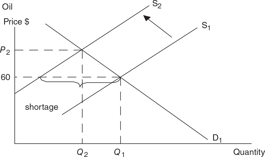
Figure 6.11

• When supply increases, equilibrium price decreases and quantity increases.
• When supply decreases, equilibrium price increases and quantity decreases.
Simultaneous Changes in Demand and Supply
When both demand and supply change at the same time, predicting changes in price and quantity becomes a little more complicated. An example should illustrate how you need to be careful.
An extremely cold winter results in a higher demand for energy such as natural gas. At the same time, environmental safeguards and restrictions on drilling in protected wilderness areas have limited the supply of natural gas. An increase in demand, by itself, creates an increase in both price and quantity. However, a decrease in supply, by itself, creates an increase in price and a decrease in quantity. When these forces are combined, we see a double whammy on higher prices. But when trying to predict the change in equilibrium quantity, the outcome is uncertain and depends upon which of the two effects is larger.
“Use different colored pens when drawing multiple curves on a single graph. This helps keep things clear when you shift many curves at a time.”
—Jake, AP Student
One possible outcome is shown in Figure 6.12, where the initial equilibrium outcome is labeled E1. A relatively large increase in demand with a fairly small decrease in supply results in more natural gas being consumed. The new equilibrium outcome is labeled E2.
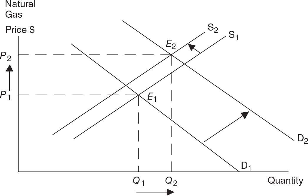
Figure 6.12
The other possibility is that the increase in demand is relatively smaller than the decrease in supply. This is seen in Figure 6.13, and, while the price is going to increase again, the equilibrium quantity is lower than before.
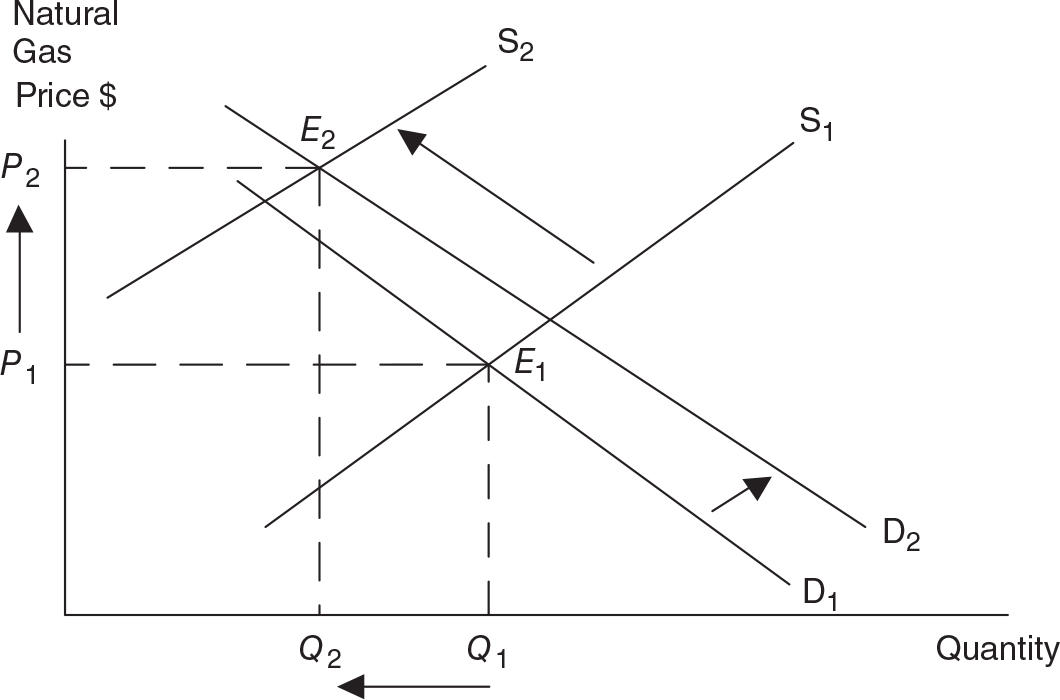
Figure 6.13

• When both demand and supply are changing, one of the equilibrium outcomes (price or quantity) is predictable and one is ambiguous.
• Before combining the two shifting curves, predict changes in price and quantity for each shift, by itself.
• The variable that is rising in one case and falling in the other case is your ambiguous prediction.
“If you don’t know the answer, it is probably where the sticks cross.”
—Chuck, AP Student
6.4 Welfare Analysis
Main Topics: Total Welfare, Consumer Surplus, Producer Surplus
Total Welfare

The competitive market, free of government and externalities, produces an equilibrium outcome that provides the maximum amount of total welfare for society. Society consists of all consumers and all producers, and, in the marketplace, each party seeks the other so that they can make an acceptable transaction at the going market price. Each party expects to gain in these transactions. Total welfare is the sum of two measures of these gains: consumer surplus and producer surplus. Some textbooks, perhaps even the one you have used, refer to this sum of consumer and producer surplus as “total surplus.”
Consumer Surplus
You know that great feeling you get when you pay a price that is lower than you expected, or is lower than you were willing to pay? That’s consumer surplus, the difference between your willingness to pay and the price you actually pay. The market demand curve, at each quantity, measures society’s marginal benefit, or willingness to pay (the price). You can see consumer surplus in Figure 6.14. At a price of $5, three units of the good are purchased. The first two units receive some amount of consumer surplus because the willingness to pay exceeds $5. The consumer of the third unit pays a price exactly equal to his willingness to pay so he earns no consumer surplus. Total consumer surplus is the total amount earned by these three consumer transactions.
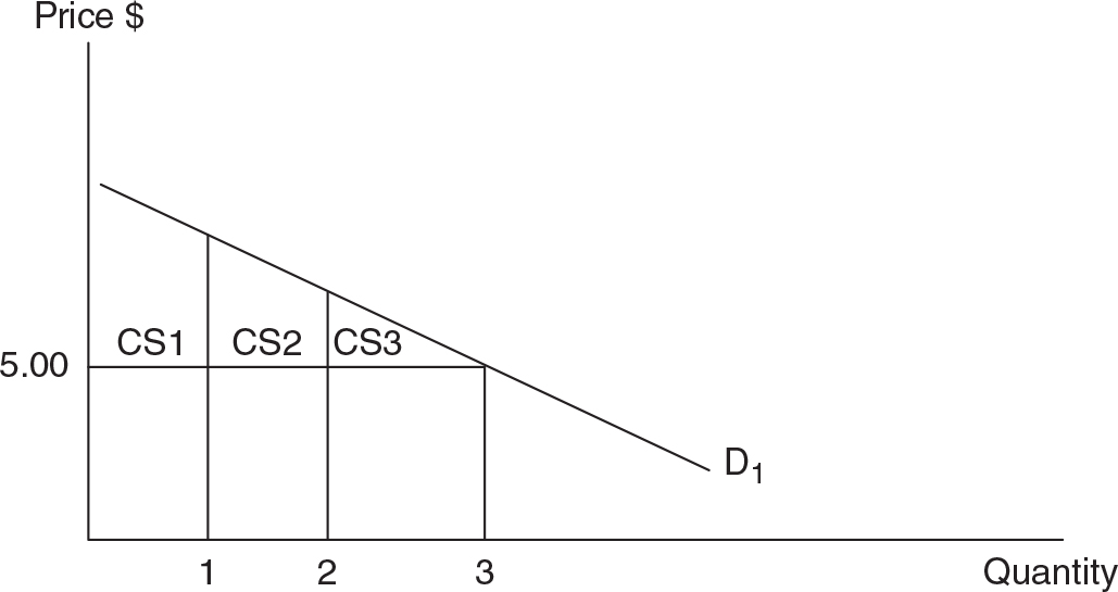
Figure 6.14
Producer Surplus
Producers are ecstatic when they receive a price for their product that is above the marginal cost of producing it. This is producer surplus, the difference between the price received and the marginal cost of producing the good. The market supply curve, at each quantity, measures society’s marginal cost. You can see producer surplus in Figure 6.15. At a price of $5, three units of the good are produced. The first two units earn producer surplus because $5 is above the marginal cost. The third unit earns no additional producer surplus, since the marginal cost is exactly equal to the price received. Total producer surplus is the total amount earned by these three producer transactions.
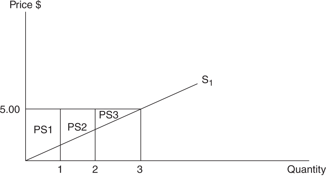
Figure 6.15

• The area under the demand curve and above the market price is equal to total consumer surplus.

• The area above the supply curve and below the market price is equal to total producer surplus.
So, is market equilibrium conducive to increasing total welfare for society? Combining Figures 6.14 and 6.15 completes the market pictured in Figure 6.16. We see that the combined consumer and producer surplus, or total welfare, is greatest at the equilibrium price of $5 and quantity of three units.
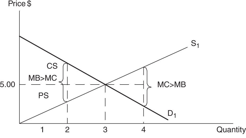
Figure 6.16
At a lesser quantity (e.g., two units), the combined area is smaller than at a quantity of three. At greater quantities (i.e., q = 4) the price of $5 exceeds MB, so consumer surplus is being lost. If this weren’t bad enough, the MC exceeds the price at q = 4, so producer surplus is being lost. Thus, if total welfare is falling at quantities less than three and at quantities greater than three, total welfare must be maximized at the market equilibrium quantity of three and price of $5.

A little bit of math can be a big help! Although the AP Microeconomics exam does not allow you to use a calculator, there are times when you will be required to do mathematical computations to earn points. In recent years, free-response questions have asked students to compute the area of consumer or producer surplus. It’s really as simple as computing the area of a triangle: ½ × base × height. Typical exam questions will provide enough information for you to see the dimensions of the triangle (base and height) and then perform the multiplication. Let’s see how this is done in the following graph.
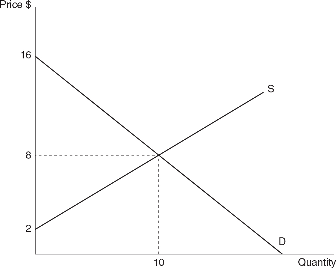
Suppose you were given this graph on a free-response question. Could you identify and compute the areas of consumer and producer surplus? It’s important to remember that the consumer surplus is the area of the triangle below the demand curve and above the market price, whereas producer surplus is the area of the triangle above the supply curve and below the market price. Of course, both of these areas also depend on the equilibrium quantity, which will be the same for both triangles. Using the numbers from the graph, we compute as follows:

You can now handle any similar questions on your exam.
 Review Questions
1. When the price of pears increases, we expect the following:
(A) Quantity demanded of pears rises.
(B) Quantity supplied of pears falls.
(C) Quantity demanded of pears falls.
(D) Demand for pears falls.
(E) Supply of pears rises.
2. If average household income rises and we observe that the demand for pork chops increases, pork chops must be
(A) an inferior good.
(B) a normal good.
(C) a surplus good.
(D) a public good.
(E) a shortage good.
3. Suppose that aluminum is a key production input in the production of bicycles. If the price of aluminum falls, and all other variables are held constant, we expect
(A) the demand for aluminum to rise.
(B) the supply of bicycles to rise.
(C) the supply of bicycles to fall.
(D) the demand for bicycles to rise.
(E) the demand for bicycles to fall.
4. The market for denim jeans is in equilibrium, and the price of polyester pants, a substitute good, rises. In the jean market
(A) supply falls, increasing the price and decreasing the quantity.
(B) supply falls, increasing the price and increasing the quantity.
(C) demand falls, increasing the price and decreasing the quantity.
(D) demand rises, increasing the price and increasing the quantity.
(E) supply and demand both fall, causing an ambiguous change in price but a definite decrease in quantity.
5. The apple market is in equilibrium. Suppose we observe that apple growers are using more pesticides to increase apple production. At the same time, we hear that the price of pears, a substitute for apples, is rising. Which of the following is a reasonable prediction for the new price and quantity of apples?
(A) Price rises, but quantity is ambiguous.
(B) Price falls, but quantity is ambiguous.
(C) Price is ambiguous, but quantity rises.
(D) Price is ambiguous, but quantity falls.
(E) Both price and quantity are ambiguous.
6. The competitive market provides the best outcome for society because
(A) consumer surplus is minimized, while producer surplus is maximized.
(B) the total welfare is maximized.
(C) producer surplus is minimized, while consumer surplus is maximized.
(D) the difference between consumer and producer surplus is maximized.
(E) the total cost to society is maximized.
 Answers and Explanations
1. C—If the price of pears rises, either quantity demanded falls or quantity supplied rises. Entire demand or supply curves for pears can shift, but only if an external factor, not the price of pears, changes.
2. B—When income increases and demand increases, the good is a normal good. Had the demand for pork chops decreased, they would be an inferior good.
3. B—This is a determinant of supply. If the raw material becomes less costly to acquire, the marginal cost of producing bicycles falls. Producers increase the supply of bicycles. Recognizing this as a supply determinant allows you to quickly eliminate any reference to a demand shift.
4. D—When a substitute good becomes more expensive, the demand for jeans rises, increasing price and quantity.
5. C—Increased use of pesticides increases the supply of apples. If the price of a substitute increases, the demand for apples increases. Combining these two factors predicts an increase in the quantity of apples, but an ambiguous change in price. To help you see this, draw these situations in the margin of the exam.
6. B—When competitive markets reach equilibrium, no other quantity can increase total welfare (consumer + producer surplus). Total welfare is maximized at that point.
 Rapid Review
Law of demand: Holding all else equal, when the price of a good rises, consumers decrease their quantity demanded for that good.
All else equal: To predict how a change in one variable affects a second, we hold all other variables constant. This is also referred to as the “ceteris paribus” assumption.
Absolute (or money) prices: The price of a good measured in units of currency.
Relative prices: The number of units of any other good Y that must be sacrificed to acquire the first good X. Only relative prices matter.
Substitution effect: The change in quantity demanded resulting from a change in the price of one good relative to the price of other goods.
Income effect: The change in quantity demanded that results from a change in the consumer’s purchasing power (or real income).
Demand schedule: A table showing quantity demanded for a good at various prices.
Demand curve: A graphical depiction of the demand schedule. The demand curve is downward sloping, reflecting the law of demand.
Determinants of demand: The external factors that shift demand to the left or right.
Normal goods: A good for which higher income increases demand.
Inferior goods: A good for which higher income decreases demand.
Substitute goods: Two goods are consumer substitutes if they provide essentially the same utility to the consumer. A Honda Accord and a Toyota Camry might be substitutes for many consumers.
Complementary goods: Two goods are consumer complements if they provide more utility when consumed together than when consumed separately. Cars and gasoline are complementary goods.
Law of supply: Holding all else equal, when the price of a good rises, suppliers increase their quantity supplied for that good.
Supply schedule: A table showing quantity supplied for a good at various prices.
Supply curve: A graphical depiction of the supply schedule. The supply curve is upward sloping, reflecting the law of supply.
Determinants of supply: One of the external factors that influences supply. When these variables change, the entire supply curve shifts to the left or right.
Market equilibrium: Exists at the only price where the quantity supplied equals the quantity demanded. Or, it is the only quantity where the highest price consumers are willing to pay is exactly the lowest price producers are willing to accept.
Shortage: Also known as excess demand, a shortage exists at a market price when the quantity demanded exceeds the quantity supplied. The price rises to eliminate a shortage.
Disequilibrium: Any price where quantity demanded is not equal to quantity supplied.
Surplus: Also known as excess supply, a surplus exists at a market price when the quantity supplied exceeds the quantity demanded. The price falls to eliminate a surplus.
Total welfare: The sum of consumer surplus and producer surplus. The free market equilibrium provides maximum combined gain to society. This is also called total surplus.
Consumer surplus: The difference between your willingness to pay and the price you actually pay. It is the area below the demand curve and above the price.
Producer surplus: The difference between the price received and the marginal cost of producing the good. It is the area above the supply curve and under the price.