CHAPTER 9
Market Structures, Perfect Competition, Monopoly, and Things Between
IN THIS CHAPTER
Summary: Chapter 7 presented the relationship between product demand, elasticity, and total revenue. Chapter 8 introduced the concept of economic profit and presented the theory behind production and costs. This chapter puts revenue and cost together to examine how a firm chooses the profit-maximizing level of output and price of the product. But this profit-maximizing decision depends very much upon the structure in which the firm operates. At one extreme there are many perfectly competitive firms, each too small to have a measurable impact on market price, much less each other. At the other extreme there is one firm, a monopolist, that absolutely controls the industry price and output. In between are various shades of each extreme, some closer to monopoly, and some closer to perfect competition. It is important to realize that there is no “representative” industry, or market structure, so we focus on four general models and study how firms in these structures determine price and output. In addition to the extremes of perfect competition and monopoly, we cover the models of monopolistic competition and oligopoly. This chapter also introduces you to some basic game theoretic models.


Key Ideas
 Perfect Competition
 Monopoly
 Monopolistic Competition
 Oligopoly
9.1 Perfect Competition
Main Topics: Structural Characteristics of Perfect Competition, Demand for the Firm, Profit Maximization, Short-Run Profit and Loss, Decision to Shut Down, Long-Run Adjustment
Structural Characteristics of Perfect Competition

Each market structure is defined by structural characteristics. These characteristics determine, among other things, how the profit-maximizing price and quantity are set in the short run, as well as how profits might be maintained in the long run. Perfect competition is typically described by four characteristics:
• Many small independent producers and consumers. Each firm is too small to have an impact on market price. No one firm can drive up the price by restricting supply, or drive down the price by flooding the market with output. No one consumer can, by changing the amount of the good that he consumes, impact the price.
• Firms produce a standardized product. There exist no real differences between one firm’s output and the next.
• No barriers to entry or exit. There exist no significant obstacles to the entry of new firms into, or the exit of existing firms out of, this industry. Profitability, or lack thereof, determines whether the industry is expanding or contracting.
• Firms are “price takers.” This characteristic is actually a result of the first three. Because all firms are too small to affect the price, they must accept the market price and produce as much as they wish at that price. Even if they could change the price, they would not do so. To see this, suppose that the market determined the competitive price of barley is $5. If farmer Katie increased the price to $5.01, she would now be the high-price supplier of barley, with thousands of competitors producing an identical product at a lower price; Katie is likely to lose all of her customers. If she lowers her price to $4.99, she would seemingly clean up her competition. But, remember, the price-taking characteristic tells us that Katie can sell all she wants at the market price of $5. If you can sell all you want at $5, why would Katie sell even one unit at $4.99?
“In order to keep the different types of firms straight, make a table including the firm’s definition, what kind of product they produce, barriers, and how they control price. It is the best way to study.”
—Kristy, AP Student
All four of the characteristics of perfect competition are rarely found in today’s industries, but agricultural commodities are usually regarded as approximately perfectly competitive.
Demand for the Firm
Each perfectly competitive firm produces a standardized, or homogenous, product. Because each firm’s output is such a small share of the total market supply, the demand for each firm’s output is perfectly elastic. Perfectly competitive firms have no effect on the market price; they simply produce as much as they can at the going price. This implies a horizontal demand curve for their product. This does not imply that the market demand curve is horizontal. If the market price of barley falls, quantity demanded rises. Figure 9.1 illustrates the difference between market demand (D) and the demand for one firm’s product (d).
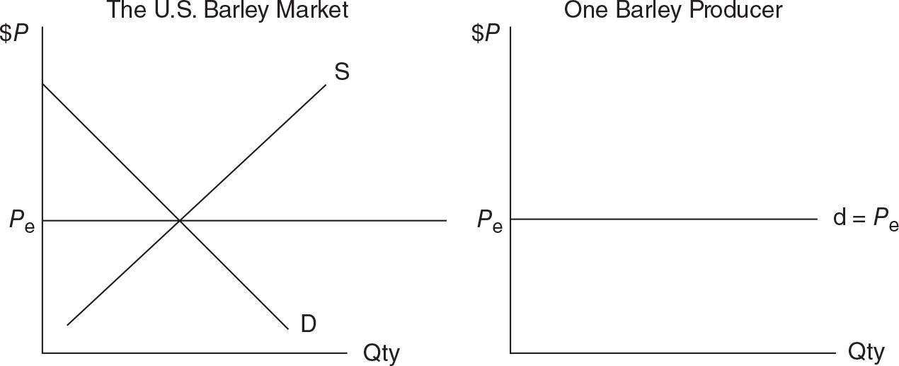
Figure 9.1
Profit Maximization

Let’s get one thing straight. When we say firms maximize economic profit, this means they are not going to settle for anything less than the highest possible difference between total revenue and total economic cost. If an additional dollar of profit is to be earned, they take that opportunity. If the maximum profit possible is actually zero, or even negative dollars, they accept this short-run outcome. There are two equivalent ways to maximize economic profit.
The Method of “Totals’’
The perfectly competitive firm cannot change the price; it can only adjust output. To maximize profit, the firm selects the output to maximize:

An example should help to illustrate how a firm goes about maximizing profit.
Example:
A carrot farmer operates in a perfectly competitive market. The going price for a bushel of carrots is $11. Table 9.1 summarizes how total revenue, total cost, and profit differ at various levels of output. Because it is the short run, there exist $16 of fixed costs. All costs reflect the explicit and implicit costs of hiring a resource.
Table 9.1

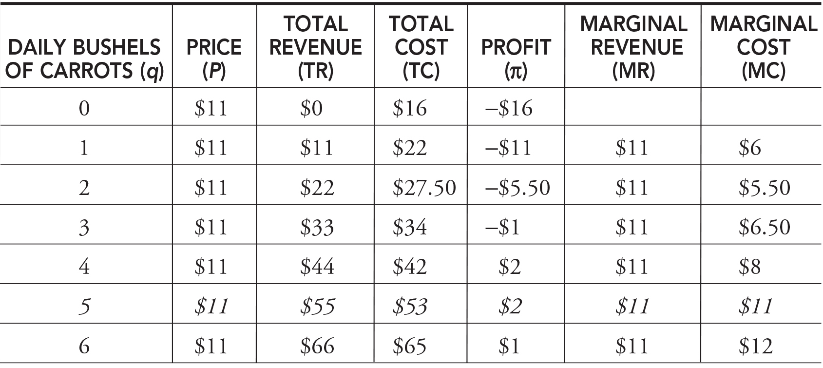
Because the firm is a price taker, the level of output does not affect the going price. Total costs rise as production increases, a concept seen in the previous chapter. As a profit maximizer, our carrot farmer would choose to produce five bushels per day and earn $2 in daily economic profit. Note, when there are two quantities that produce the same amount of profit, like four and five bushels, we select the larger of the two quantities. This method of profit maximization is much like trial and error and is a bit cumbersome. Let’s explore an equivalent and easier way.
The Method of “Marginals”
Throughout this book we have seen illustrations of marginal analysis, and this situation is no different. You’ll recall that rational decision making implies the following:

• If MB > MC, do more of it.
• If MB < MC, do less of it.
• If MB = MC, stop here.
Since the only decision to be made by the perfectly competitive firm is to choose the optimal level of output, the firm’s rule is as follows:

• Choose the level of output where MR = MC.
Table 9.2 can be modified to show the marginal revenue and marginal cost of selling additional bushels of carrots.
Table 9.2
“Keep answers crisp, graphs labeled, and you are on your way to a 5.”
—Navin, AP Student
Notice that in perfect competition, the price is equal to marginal revenue. This is fairly simple if you recall the assumptions of the model. Farmers can sell as much as they want at the market price. If a farmer sells one more bushel, total revenue increases by the price of the bushel, $11 in this case. Sell another bushel; earn another marginal revenue of $11. Price is also equivalent to average revenue (AR), or total revenue per unit. These relationships can be seen in Figure 9.2.
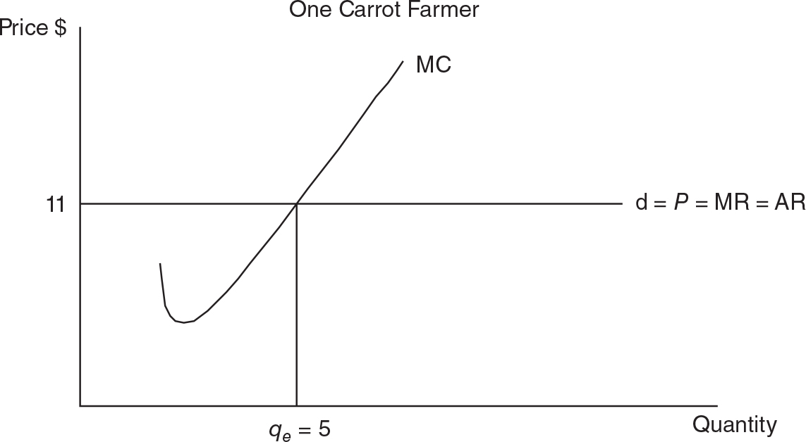
Figure 9.2

• MR = ΔTR/ΔQ = P × ΔQ/ΔQ = P
• AR = TR/Q = P × Q/Q = P
• P = MR = AR = Demand for the firm’s product
• Total revenue (P × q) equal to $55 can be seen as the area of the rectangle with a height of P = $11 and width of qe = 5.
Short-Run Profit and Loss
To maximize profit, the firm must choose the level of output (qe) where MR = MC. But how can we use Figure 9.2 to identify these profits? A little algebra goes a long way.
π = TR - TC = P × qe - TC. If you divide both terms by quantity and remember that TC/q = Average total cost (ATC), you have

The term (P - ATC) is the per-unit difference between what the firm receives from the sale of each unit and the average cost of producing it, or profit per unit. When you multiply this per-unit profit by the number of units (qe) produced, you have total profit. Table 9.3 and Figure 9.3 incorporate the ATC into our carrot farmer’s profit-maximizing decision table.
Table 9.3


Figure 9.3
Profit Rectangles and Flying Monkeys
“This is a great analogy to remember.”
—AP Teacher
Everyone remembers The Wizard of Oz and the critical instructions that the people of Munchkinland gave Dorothy and Toto as they set off to find the Wizard: “Follow the yellow brick road.” And when Dorothy, Toto, and friends stayed on the yellow brick road, they were fine. Whenever they ignored these cautionary words and left the yellow brick road, bad things happened—the scariest being the arrival of the flying monkeys. The flying monkeys tore the Scarecrow limb from limb and set the Scarecrow’s straw innards on fire. Very bad things happen when you leave the yellow brick road.
When you find the profit-maximizing level of production, qe, you are locating the yellow brick road for this firm. Never leave this level of output or bad things happen. Finding qe is the first step in calculating profit with a “profit rectangle.” The area of the shaded rectangle is 5 bushels wide, multiplied by 40 cents high. In our case, the price $11 in Figure 9.3 is above the average total cost $10.60, so we have positive economic profits of $2. This does not always occur in the short run. Another look at our per-unit equation tells us:

• If P > ATC, π > 0.
• If P < ATC, π < 0.
• If P = ATC, π = 0.
Short-Run Losses
While firms would love to maintain the above scenario where P > ATC and positive economic profits are made, it might not always turn out that way. Due to a failure of the Bugs Bunny diet fad, the market for carrots suffers a dramatic decrease in demand. Plummeting demand decreases the market price to $6.50 per bushel, and firms must readjust their profit-maximizing output decision.
As seen in Table 9.4, at the much lower price of $6.50, the firm now finds that MR = MC at an output of three bushels per day. Not surprisingly, the opportunity for positive economic profit has been eliminated. The profit-maximizing, or loss-minimizing, output of three bushels provides the best possible scenario for the firm; but that scenario involves economic losses of $14.50. The rectangle can still be seen in Figure 9.4, where average total cost is $11.33 per bushel.
Table 9.4

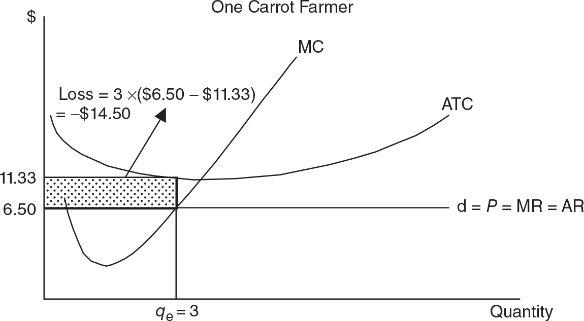
Figure 9.4

• Many AP students lose points because they incorrectly locate and label profit. When you are finding the profit/loss rectangle, it is important to remember the following.
• Find qe where P = MR = MC. Once you have found qe, never leave it.
• Find ATC vertically at qe. If you move downward, π > 0. If you move upward, π < 0.
• Move horizontally from ATC to the y-axis to complete the rectangle, and clearly label it as positive or negative.
Decision to Shut Down

Firms obviously do not enjoy producing at a loss and desperately hope that the market price improves so that profits are possible. However, if firms are incurring losses, they must decide whether it is economically rational to operate at all. The decision to shut down, or produce zero, in the short run is sometimes the optimal strategy. To see why, consider what happens when a firm begins to produce. When a perfectly competitive firm decides to produce any level of output greater than zero, two things happen.
“This has great potential to be asked on both sections of the exam.”
—AP Teacher
1. It collects total revenue (TR) = P × qe.
2. It incurs variable costs (TVC). Of course, the firm also incurs total fixed costs, but it incurs those costs anyway, regardless of the level of output.
“If you only remember one thing, remember this! MR = MC.”
—Kristy, AP Student
If the firm, by producing in the short run, can collect total revenues that at least exceed the total variable costs, then it continues to produce, even at a loss. However, if producing output incurs more variable cost than revenue collected, why bother? Shut down, hope for better times, and suffer losses equal to TFC. This comparison provides us a decision rule for shutting down in the short run:

• If TR ≥ TVC, the firm produces qe where MR = MC.
• If TR < TVC, the firm shuts down and q = 0.
The Shutdown Point
We can see the shutdown point in Figure 9.5 by converting the above decision rule into a per-unit comparison. Dividing total revenue and total variable cost by q tells us to shut down if P < AVC. This is the identical decision rule; it is just a per-unit comparison of revenue and variable cost:
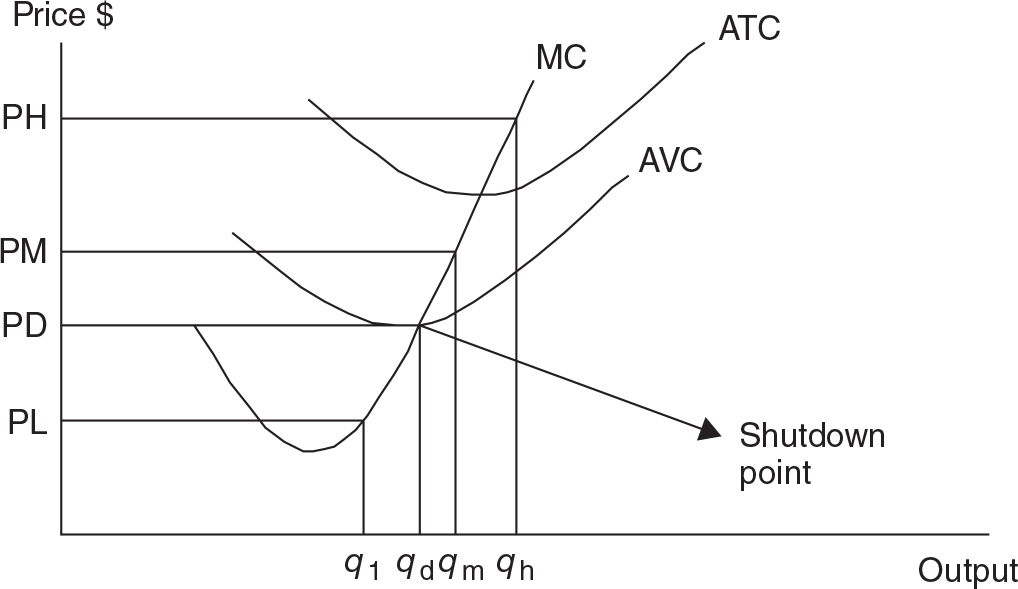
Figure 9.5

• If P ≥ AVC, the firm produces qe where MR = MC.
• If P < AVC, the firm shuts down and q = 0.
In Figure 9.5, there are four prices shown:
• PH is the highest price. At qh, the firm earns enough total revenue to cover all costs. π > 0.
• PM is the middle price. At qm, the firm’s TR exceeds TVC but only covers part of the TFC. π < 0.
• PD is the shutdown price. At qd, the firm’s TR just covers TVC and the firm is at the shutdown point. If price falls any lower, the firm does not produce.
• PL is the lowest price. At q1, the firm’s TR cannot even cover TVC, and so the firm shuts down, producing q = 0. π = -TFC.
Short-Run Supply
As you can see in Figure 9.5, when the price fluctuates between PH and PD, the firm finds a new profit-maximizing quantity where P = MR = MC. If price increases, quantity supplied increases. If price decreases, quantity supplied decreases. This is a restatement of the law of supply. This movement upward and downward along the marginal cost curve implies that MC serves as the supply curve for the perfectly competitive firm. The only exception is when the price falls below the shutdown point (minimum of AVC) and the firm quickly decides to produce nothing. The market supply curve is simply the horizontal summation of all firms’ MC curves.
• The MC curve above the shutdown point serves as the supply curve for each perfectly competitive firm.
• The market supply curve is therefore the horizontal sum of all of the MC curves: S = S MC.
Long-Run Adjustment

The short run is a period of time too brief for firms to change the size of their plants. This means that it is also too short for existing firms to exit the industry in bad times and too short for new entrepreneurs to enter the industry in good times. The “free entry and exit” characteristic of perfect competition assures us that in the long run, we can expect to see firms either exiting or entering, depending upon whether profits or losses are being made in the short run. We’ll first examine the case where short-run positive profits are made in the carrot industry. Then we’ll look at the situation where short-run losses are incurred.

• In most of the past AP Microeconomics exams, free-response questions have appeared that test the students’ knowledge of perfect competition and the difference between the short- and long-run equilibria.
Short-Run Positive Profits
Figure 9.6 illustrates the perfectly competitive carrot industry where the market price is above average total cost. Firms are earning positive short-run profits, as illustrated by the shaded rectangle.
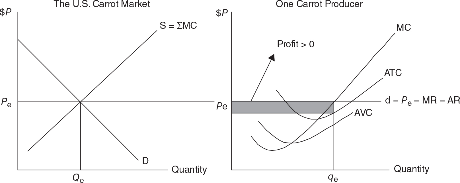
Figure 9.6
So what next? Well, many entrepreneurs on the outside of this market are attracted by the positive short-run profits being made by carrot producers. Given sufficient time (i.e., the long run), these new firms enter the market. With more carrot producers, the market supply curve shifts outward, driving down the price. As the price falls, the profit rectangle gets smaller and smaller until it actually disappears. At the point where P = MR = MC = ATC, each carrot farmer is now breaking even with π = 0. Would the next potential carrot farmer enter the market? Unlikely, as the entry of one more firm pushes the price down just enough to where losses are actually incurred. Thus, this breakeven point is described as the long-run equilibrium. The market quantity has increased, and each firm produces less at the lower price. Figure 9.7 illustrates the movement toward the long-run equilibrium.
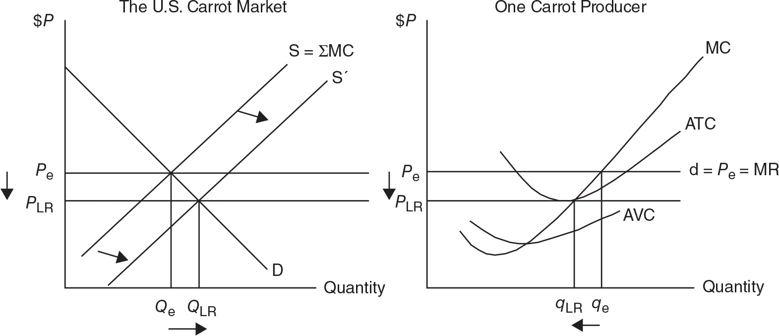
Figure 9.7

• Entry of new firms attracted by economic π > 0.
• Increase in market supply.
• A decrease in the market price to PLR.
• Profits fall to the breakeven point, PLR = MR = MC = ATC and economic π = 0.
• Market quantity increases.
• Individual producer output falls.
• Many FRQs ask you to draw perfect competition with side-by-side graphs of the market and the typical firm. In addition to knowing perfect competition inside and out, you must be very careful to follow all instructions in the prompt. For example, questions often say, “Label output in the market Qm and output for the typical firm Qf.” Following these instructions exactly can prevent unnecessary errors that will cost you easy graphing points.
What’s So Great About Breaking Even?
Remember there is a distinction between accounting profit and economic profit. Economic profit subtracts the next best opportunity costs of your resources from total revenue. If you are still breaking even after subtracting what you might have earned in all of those other opportunities, you can’t feel cheated. In other words, you are making a fair rate of return on your invested resources and you have no incentive to take them elsewhere. Sure, you would like to earn more than zero economic profit (aka “normal profit”), but the characteristics of perfect competition rule this out in the long run.
Short-Run Losses
Figure 9.8 illustrates short-run losses with a price below ATC but above the shutdown point. The long-run adjustment story might sound familiar, only with market forces moving in the opposite direction.
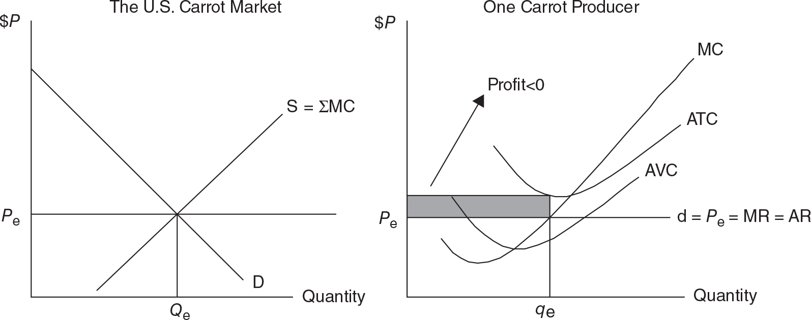
Figure 9.8
Again, we should ask “What next?” Some existing firms in this market begin to exit the industry. With fewer carrot producers, the market supply curve shifts leftward, driving up the price. As the price rises, the loss rectangle gets smaller and smaller until again it disappears. At the point where PLR = MR = MC = ATC, each remaining carrot farmer is now breaking even with P = 0. Would another carrot farmer exit the market? Possibly, but the exit of one more firm bumps up the price just enough so that a small positive profit is earned, prompting one firm to enter and get us back to the breakeven point. Arrival at the breakeven point is once again the long-run equilibrium. The market quantity has decreased, but each surviving firm produces more at the higher price. Figure 9.9 illustrates the movement toward the long-run equilibrium.

Figure 9.9
The long-run adjustment to short-run losses can be summarized as:

• Exit of existing firms prompted by economic π < 0.
• Decrease in market supply.
• An increase in the market price to PLR.
• Profits increase to the breakeven point, PLR = MR = MC = ATC and economic π = 0.
• Market quantity decreases.
• Individual producer output rises.
Table 9.5 provides a summary of the four possible short-run scenarios and resulting long-run adjustments to the perfectly competitive equilibrium, which always ends in the same place.

Table 9.5

Are There Variations on This Story and Do I Need to Know Them?
The answer to these questions are yes, and maybe. Throughout this section we have made an assumption that entry and exit of firms has no impact on the cost curves of firms in the market. In other words, we have been assuming a constant cost industry. Recent AP Microeconomics exams have made references to constant cost industries and (maybe) caused unnecessary confusion for test takers. It is always possible that future exams will refer to constant, increasing, or decreasing cost industries, so you should probably become familiar with these terms. A quick explanation and you will not be one of the confused.
Suppose that entry of new firms into a profitable carrot market increases the demand for key resources like land, labor, and capital. Increased demand for these resources might increase the cost of employing those resources. When this happens, the cost curves for firms in the carrot industry start to shift upward. This situation is described as an increasing cost industry. Graphing this situation gets sticky, but if you follow the logic, you will be fine. The entry of new firms drives down the price of the output and increases the cost curves, so the profit is eliminated more quickly than with our constant cost industry. Fewer firms eventually enter this version of the carrot market, and the new long-run price is higher than it is in a constant cost industry.
A decreasing cost industry is one in which the entry of new firms actually decreases the price of key inputs and causes the cost curves to shift downward. This might occur because producers of the key inputs expand production and experience economies of scale and lower per-unit costs. Since the entry of new firms lowers the price of the output and decreases the cost curves, it takes longer for the profit to be eliminated than in our constant cost industry. More firms can eventually enter this market, and the new long-run price is lower than it would be in a constant cost industry.
9.2 Monopoly
Main Topics: Structural Characteristics of Monopoly, Monopoly Demand, Profit Maximization, Efficiency Analysis, Price Discrimination
Structural Characteristics of Monopoly

Since monopoly is the very opposite of perfect competition in the range of market structures, we can expect that the structural characteristics are also quite different.
• A single producer. This is pretty self-explanatory, but a strict definition of monopoly requires that there are no other firms in the industry.
• No close substitutes. Consumers cannot find a similar product in other markets.
• Barriers to entry. Perhaps the most important characteristic of monopoly is that there exists something that prevents rival firms from entering the market to provide competition to the monopolist and choice to consumers.
• Market power. This is the result of the first three characteristics. With no competition and barriers to entry, the unregulated monopolist has market power, or monopoly price-setting ability.
Again, it is rare to find a firm that satisfies all of the characteristics of monopoly, but the De Beers firm holds a near monopoly on global diamond production. The only gas station or bank in a small town might also act as a local monopolist.
Barriers to Entry
If there were no barrier to entry, a monopolist earning positive economic profits would be history and this chapter would be done. So before moving on to the behavior of monopoly, let’s talk a little more about this necessary condition for the existence of monopoly.
• Legal barriers. In your local television market, only one firm is given the right to broadcast on a specific frequency. There might be only one firm given the right to sell liquor in a small community. There are patents, trademarks, and copyright laws to protect inventions and intellectual property. These legal protections do not provide for absolute monopoly, for there are often viable substitutes available to consumers.
• Economies of scale. In Chapter 8 this concept was introduced. As a firm grows larger in the long run, average total costs fall, providing the larger firm a cost advantage over smaller firms. If extensive economies of scale exist, an industry could evolve into one with only one enormous producer. A natural monopoly is a case where economies of scale are so extensive that it is less costly for one firm to supply the entire range of demand. Power plants are a good example of natural monopoly within a local area.
• Control of key resources. If a firm controlled most of the available resources in the production of a good, it would be very difficult for a competitor to enter the market. For example, if a producer of granulated sugar wanted to monopolize the market, the firm might wish to control all of the sugarcane plantations.
Monopoly Demand
The perfectly competitive firm is a price taker and faces perfectly elastic demand for the product. The firm sells all it wants at the going market price; this decision does not affect the market price. The monopolist is the only provider of that good, making the demand for the product the market demand for that product. The monopolist must pay attention to the law of demand, which means that if it wishes to sell more, the monopolist must decrease the price.
Demand, Price, and Marginal Revenue
Price exceeds marginal revenue because the monopolist must lower price to boost sales. The added revenue from selling one more unit is the price of the last unit less the sum of the price cuts that must be taken on all prior units of output. For example, the demand curve for the monopolist’s product is P = 7 - Qd.
The monopolist begins at a price of $6 and sells one unit of the good (see Table 9.6). A price cut to $5 results in one more unit sold, so total revenue increases by $5 on this second unit. However, the first unit, previously sold at $6, must also now be sold at $5, which costs the firm $1 in total revenue. With $5 gained (P) from the second and $1 lost in total revenue from the first unit, the net or marginal increase (MR) in total revenue is $4 for the second unit. Graphically we can see the revenue effect of selling the second unit in Figure 9.10.
Table 9.6
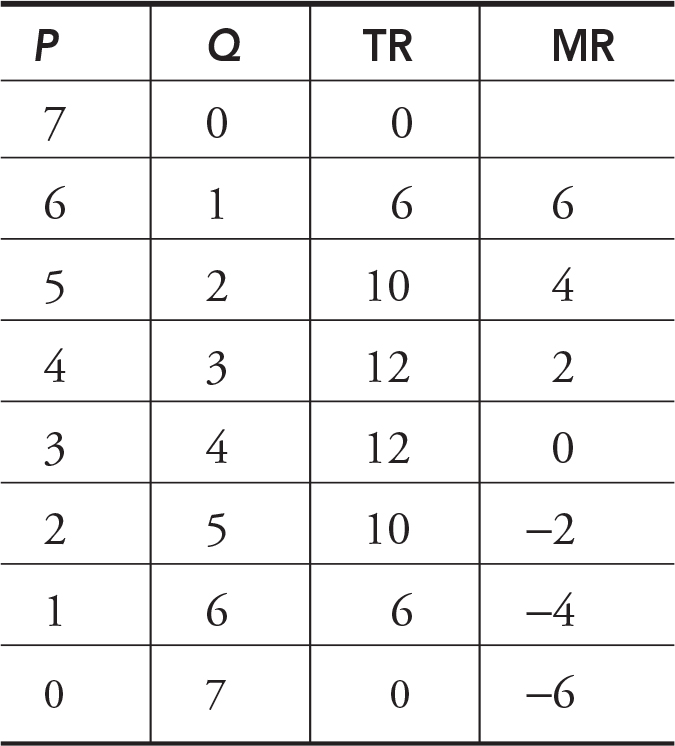
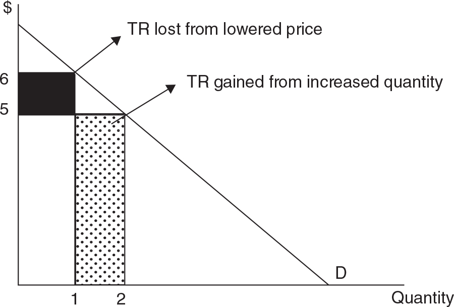
Figure 9.10

Chapter 7 examined the effect that price elasticity of demand (Ed) has on total revenue. Demand is elastic above the midpoint of a linear demand curve like the one in Figure 9.10, so cuts in price increase total revenue. Demand is inelastic below the midpoint; further cuts in price decrease total revenue. At the midpoint, total revenue is maximized and demand is unit elastic. Recognizing this connection, the price-making monopolist is going to avoid the inelastic portion of the demand curve and operate at some point to the left of the midpoint. Figure 9.11 combines demand, marginal revenue, and the total revenue function. You can see that when total revenue is at the maximum, marginal revenue is zero and further price cuts decrease total revenue, making marginal revenue negative.

Figure 9.11

• Demand is horizontal, and P = MR in perfect competition.
• Demand is downward sloping, and P > MR in monopoly.
• The monopolist operates in the elastic (or upper) range of demand.
Profit Maximization

While demand looks different for the monopolist, the mechanism for maximizing profit is the same for both the monopolist and the perfectly competitive firm. The firm must set output at the level where MR = MC. At this level of output (Qm), the monopolist sets the price (Pm) from the demand curve. Profit is found in the same way by creating the profit rectangle with average total cost. This is seen in Figure 9.12.
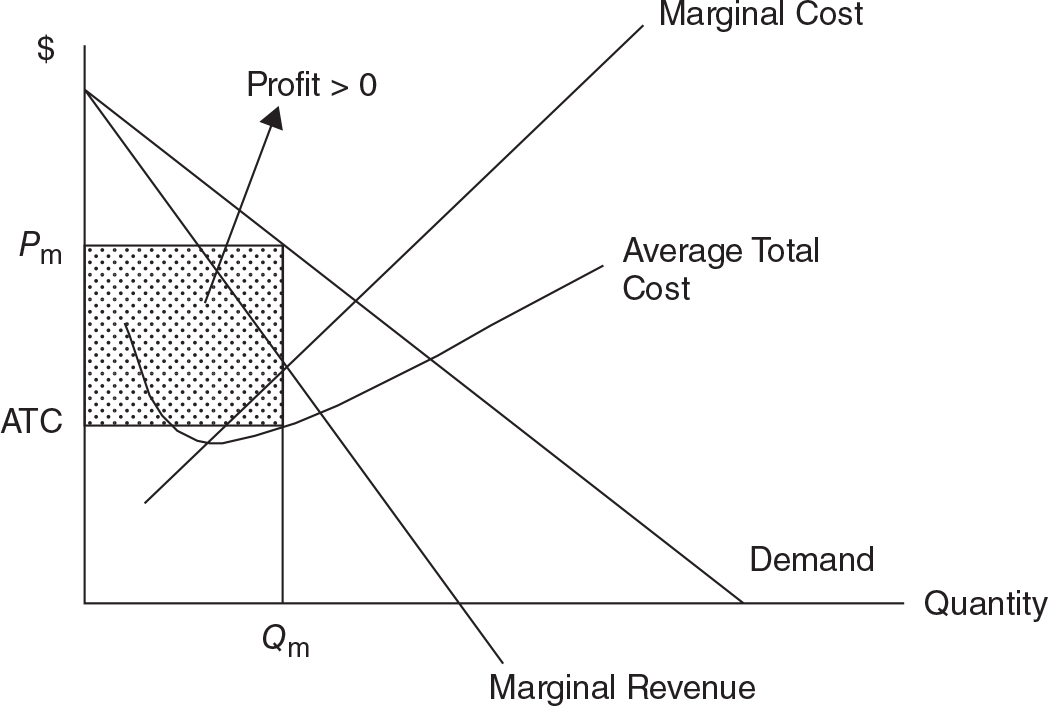
Figure 9.12
“Understand the profit max rule well. It will help you throughout economics.”
—Nick, AP Student
The positive monopoly profits illustrated in Figure 9.12 are likely, due to the entry barrier, to last into the long run. Though π > 0 is usually the case for a monopoly firm, you might imagine a case where demand plummets, or perhaps production costs increase, to the point where P < ATC and losses are incurred. In the event of persistent losses, we expect the monopolist to exit the industry.

• Find Qm where MR = MC. Once you have found Qm, never leave it.
• Find Pm vertically from the demand curve above MR = MC.
• Find ATC vertically at Qm. If you move downward, π > 0. If you move upward, π < 0.
• Move horizontally from ATC to the y-axis to complete the rectangle and clearly label it as positive or negative.
Efficiency Analysis

We refer to efficiency in a couple of different sections of this book, and now that we have compared perfect competition to monopoly, it is time for another discussion. Allocative efficiency is achieved when the market produces a level of output where the marginal cost (MC) to society exactly equals the marginal benefit (P) received by society. Total welfare to society is maximized at this outcome, so any movement away from this level of output results in deadweight loss. Productive efficiency is achieved if society has produced a level of output with the lowest possible cost. In perfect competition, the long-run market outcome achieves both of these criteria for efficiency. Figure 9.13 illustrates the competitive and monopoly outcomes. Allocative efficiency exists because Pc = MR = MC at Qc, and productive efficiency exists because firms produce at minimum ATC, once entry or exit has occurred in the long term.

Figure 9.13
On the other hand, the monopolist produces at a quantity Qm where Pm > MR = MC. This result tells us that consumers would like to consume more of the product; but the monopolist does not produce as much as consumers want. This is an example of market failure, a concept introduced back in Chapter 5. Failing to achieve allocative efficiency creates the deadweight loss (DWL) shown in Figure 9.13. The monopoly output is not at the point where ATC is minimized; thus the monopolist is not productively efficient. A profit earned by the monopolist is a transfer of consumer surplus from consumers to the firm. To see what happens to output, price, profit, and efficiency after a tax has been imposed, see one of the practice FRQs later in this book.

• Qm < Qc.
• Pm > Pc.
• Pm > MC so monopoly is not allocatively efficient.
• Deadweight loss exists with monopoly.
• Pm > minimum ATC so monopoly is not productively efficient.
• πm > 0 is a transfer of lost consumer surplus from consumers to the firm.
Price Discrimination
Though the name implies a nasty stereotype, price discrimination is the selling of the same good at different prices to different consumers. Successful price discrimination is possible if three conditions exist:
1. The firm has monopoly pricing power.
2. The firm is able to identify and separate groups of consumers.
3. The firm is able to prevent resale between consumers.
Common examples of price discrimination include the following:
• Child and senior discounts at the movie theater or restaurants
• Airline tickets that are bought three weeks in advance compared to tickets bought one hour in advance
• Coupons that separate price-sensitive consumers (those who use the coupon) from those who are less price sensitive
• A lower per-unit price paid by consumers who buy items in large quantities (like a case of soda) than those paid by consumers who buy in lesser quantities (like a six-pack of soda, or one can from a vending machine)
The airline industry is clearly not perfectly competitive, so there must be a degree of monopoly pricing power. The firm creates groupings based upon when consumers purchase tickets. The photo identification requirement for all passengers is an important security measure, but it also prevents the resale of a low-priced ticket to a consumer who is willing to pay a higher price. If resale were possible, the pricing system might break down. It should not surprise you that price discrimination allows firms to earn more profit than if they charged a single price.
Perfect Price Discrimination
Imagine a monopoly shop that sells a certain kind of gadget, but there is something odd about the way these gadgets are priced. When a customer walks into the shop, a sign above the door flashes a number that only the shopkeeper can see; this number is the highest price this particular customer is willing to pay (WTP) for a gadget. Because each customer has a different budget, and different tastes and preferences, each customer has a different WTP. The shopkeeper, knowing the customer’s willingness to pay, charges a price exactly equal to this customer’s WTP. For example, if Becky’s WTP is $8, that’s the price she would be charged for a gadget. If Jamaal’s WTP is $9.50, that’s the price he would be charged.
This unique kind of price discrimination is called perfect price discrimination and is seen in Figure 9.14. The demand curve and marginal revenue are now the same (P = MR), and the firm will continue selling gadgets until the marginal revenue from the last sale is equal to the marginal cost of a gadget. There is no single equilibrium price, because each customer was charged a different price. There are two other key outcomes to see here. First, because each customer pays a price exactly equal to their WTP, there is no consumer surplus; the monopolist takes all of it as producer surplus. Second, because the last unit sold is the one for which P = MC, this outcome is allocatively efficient.
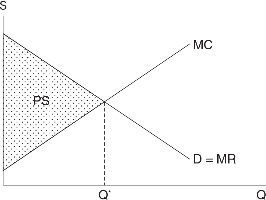
Figure 9.14
9.3 Monopolistic Competition
Main Topics: Structural Characteristics, Short-Run Profit Maximization, Long-Run Adjustment
Structural Characteristics

Sharing some of the characteristics of both perfect competition and monopoly, the market structure of monopolistic competition provides a description of many modern industries.
• Relatively large number of firms. Rather than the thousands of perfectly competitive firms, in monopolistic competition there are perhaps dozens, each with a fairly small share of the total market.
• Differentiated products. This characteristic makes monopolistic competition stand out as different from the perfectly competitive market structure and gives firms their ability to set the price above the competitive level.
• Easy entry and exit. There are very few barriers to entry in monopolistic competition, perhaps the largest being the need to provide sufficient marketing to differentiate a new firm’s product from that of the existing rivals.
The market for shoes closely fits the description of monopolistic competition. While all shoes serve the same basic purpose, to cover and protect the feet, a running shoe, a hiking boot, and a flip-flop are very different and are made by many firms in the global market. The book publishing and local restaurant markets are also described as monopolistically competitive.
Short-Run Profit Maximization
Like the monopoly, the firm in monopolistic competition faces a downward-sloping demand curve for its differentiated product. Because there are many similar substitutes available to consumers, the demand is fairly elastic. In a recurring theme for profit-maximizing behavior, the firm sets Qmc where MR = MC and sets the price from the demand curve. Figure 9.15 illustrates a monopolistically competitive firm that is earning positive short-run economic profits.
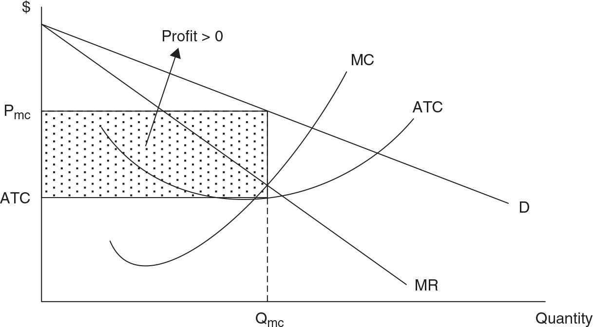
Figure 9.15
Long-Run Adjustment
With easy entry and exit into the monopolistically competitive industry, short-run positive profits like those in Figure 9.15 are not going to last for long. As new firms enter this industry, the market share of all existing firms begins to fall. Graphically we see this as a leftward shift in the demand curve. As the price begins to fall, the profit rectangle begins to shrink. Entry stops when profits are zero and Pmc = ATC, or when the demand curve is just tangent to ATC. This adjustment is seen in Figure 9.16.

Figure 9.16
“What About Advertising to Maintain Profits?”
Because easy entry of competitors drives profits down to breakeven levels, monopolistically competitive firms typically engage in extensive amounts of advertising to slow down, and even reverse, declining market share. This advertising is realistically only a short-run “fix,” as there is no reason to believe that barriers to entry suddenly emerge to prevent the eventual return to breakeven profit levels.
Efficiency and Excess Capacity
In long-run monopolistic competition, the firm earns π = 0, a characteristic shared by the perfectly competitive firm. But because of the differentiated products, P > MR = MC, allocative efficiency is not achieved. The deadweight loss is the shaded area in Figure 9.16. Though the firms are breaking even, they are not operating at the minimum of ATC; productive efficiency is also not achieved. The difference between the monopolistic competition output Qmc and the output at minimum ATC is referred to as excess capacity. Excess capacity is underused plant and equipment that is the result of producing at an output less than that which minimizes ATC. The market is overpopulated with firms, each producing enough to break even in the long run, but so many firms means that each produces below full capacity.

• Qmc < Qc.
• Pmc > Pc.
• Pmc > MC so monopolistic competition is not allocatively efficient.
• Deadweight loss exists, but not as much as with monopoly.
• Pm > minimum ATC so monopolistic competition is not productively efficient.
• πmc = 0 in the long run.
• Excess capacity is Qatc - Qmc.
9.4 Oligopoly
Main Topics: Structural Characteristics, Industry Concentration, Game Theory and the Prisoner’s Dilemma, Is Every Game a Prisoner’s Dilemma?, Collusive Pricing
Oligopoly markets are typically further from perfect competition than the monopolistic market structure, although there is no one model of oligopoly. A couple of oligopoly models are presented, but keep in mind that if one little assumption is relaxed, the predictions of the model can be radically different. For the AP exam you will likely face only these basics.
Structural Characteristics

You can see from these characteristics that oligopoly shares more common ground with monopoly, but these are flexible enough to describe many different and diverse industries:
• A few large producers. Can it get more vague than this? Think of the American auto industry, with the “Big 3” producers, or cell phone providers, an industry dominated by four huge firms. If the distribution of market share in an industry is top-heavy with a few large firms, the industry is described as oligopolistic.
• Differentiated or standardized product. Oligopoly industries can come in both flavors. Crude oil is a fairly standard product, but it is very much an oligopoly of large producers. Automobiles, beer, and soft drinks are also oligopoly markets, but with more differentiated products.
• Entry barriers. If these industries were fairly easy to enter, we would not see them dominated by a few huge producers.
• Mutual interdependence. Because a few large producers control these industries, the action of one firm (price setting or advertising) is likely to affect the others and prompt a response. A good example of this is your local gasoline market. This is very much an oligopoly; when one gas station lowers prices by one cent per gallon, the others usually quickly follow.
Industry Concentration
How does an industry become classified as an oligopoly? Economists have tried to get more specific than a “few large producers” by developing ways to measure how much market share is held by, or concentrated in, the largest of the firms. One way to gauge how powerful the largest of firms might be is to sum up the market share of the top 4, or 8, or 12 firms and create a concentration ratio. If the top four firms in the breakfast cereal industry have a combined market share of 85 percent, we say that the four-firm concentration ratio is 85. Some economists use a four-firm concentration ratio of 40 percent or greater as a rough guideline for identifying an oligopolistic industry. We predict that as this concentration ratio increases, the degree of monopoly price-setting power increases.
Game Theory and the Prisoner’s Dilemma

Imagine a case where a two-firm oligopoly (a duopoly) engages in a daily pricing decision. Each firm knows that if it sets a price higher than the rival’s, it loses sales. Likewise, if it sets a price below the rival’s, it steals sales. This noncollusive model of pricing, called the prisoner’s dilemma, emerges from the following scenario that any fan of Law and Order quickly recognizes.
Example:
A college professor suspects two students (Jack and Diane) of cheating on a take-home final exam, but she cannot prove guilt with enough certainty to fail both students in the course or expel them from the school. Without a confession, she will give each student a D in the course. With a confession from one student but not the other, she can reward the confessor with a B. The professor brings both students, one at a time, into her office and gives each the following deal:
• If you remain silent and do not confess, and your classmate implicates you, I will expel you from school and give your friend a B.
• If you confess to cheating and implicate your silent classmate, I will pass you with a B and expel your friend from school.
These options are depicted in the following matrix:

Diane doesn’t know what Jack is going to do when he is in the professor’s office. But whatever Jack’s decision, Diane should confess. She might be thinking that Jack is going to confess. If so, she confesses because staying silent will get her expelled from school. Maybe she thinks that Jack is going to stay silent. If true, the choice is between a B and a D in the course. Diane would be wise to confess. For Diane, confessing is a dominant strategy because no matter what Jack does, confession is always better than staying silent. Likewise, for Jack, the dominant strategy is to confess.
The outcome of the game (both students confess) is called a “Nash equilibrium” after the late Dr. John Nash, a mathematician at Princeton, who won the Nobel Prize in Economics in 1994. The premise is quite simple: the outcome of the game is a Nash equilibrium if each player’s strategy maximizes his or her payoff, given the strategies used by the rival players. In other words, Jack’s decision to confess ensures his best outcome, given he knows that Diane is also going to confess. And the same is true of Diane’s decision. In other words, the decision to confess is the best response to what the other player is going to do.
This is certainly a dilemma, because if Jack and Diane could only agree to give the professor the silent treatment, they would both walk away with a D, which is much better than failing the course or expulsion from school. Without such a binding agreement, cheating on the pact would be quite tempting, maybe even fairly predictable.
Example:
The owners of two gas stations operate on opposite corners of a busy intersection. Every morning each owner goes out to the sign and sets the price of gasoline, either high or low. Consumers are concerned only about the lowest price of gas. The following matrix summarizes the daily revenues for each station:

Can you see the dilemma? Both stations would love to set a high price of gas so that they could earn $2,000 in daily revenue. But if the rival were to set the low price, the high price station would be stuck with $500 while the other station cleans up with $3,000. Since both firms recognize that pricing low is the dominant strategy, both earn only $1,000 every day. This outcome, where both firms set the low price, is the Nash equilibrium. A collusive agreement might emerge.
Use of the previous game matrices assumes that both players in the game make simultaneous choices. Many games involve a series of stages where one player moves first. The second player observes the choice made by the first and then reacts to it. These sequential games are typically seen as a game tree rather than a game matrix.
Let’s convert the previous game to a sequential game where gas station X gets to move first, as shown in Figure 9.17. Station Y sees the choice of station X and then sets the price high or low. Payoffs are given at the end of the tree.

Figure 9.17
Can you see how this game will play out? Gas station X knows that its rival, station Y, still has a dominant strategy of setting a low price. No matter what the initial decision of station X, station Y would always see that a low price beats a high price. Because station X knows this about its rival, it will select a low price at the beginning of the game. In 2007, the AP Microeconomics exam included simple game theory on the free-response section for the very first time. Since 2007, this area of microeconomics has been repeatedly tested, and I predict that the degree of difficulty will gradually increase.
Is Every Game a Prisoner’s Dilemma?
Absolutely not. Several recent AP Microeconomics exams have included FRQs that are not simple examples of a prisoner’s dilemma.
Example:
Suppose there are two hamburger stands in town, Stinky’s and Sloppy’s, and each firm sells what it considers to be the best burger in town. Both burger stands are considering a move to offer hot dogs on the menu, or they could do nothing and continue to offer only burgers. The following payoff matrix shows payoffs as daily profits for Stinky’s, followed by daily profits for Sloppy’s.

In this game, Stinky’s has a dominant strategy of adding hot dogs to the menu. No matter what Sloppy’s does, Stinky’s earns more money by making this choice. However, Sloppy’s does not have a dominant strategy. If Stinky’s were to offer only burgers, Sloppy’s should add hot dogs ($400 is better than $300). But if Stinky’s were to add hot dogs to its menu, Sloppy’s should continue to offer only burgers ($200 is better than $100).
So where is the dominant strategy? Sloppy’s will recognize that Stinky’s is going to add hot dogs to the menu, so Sloppy’s will respond by maintaining a burgers-only menu. The Nash equilibrium combination of payoffs is $600 for Stinky’s and $200 for Sloppy’s. This is not a prisoner’s dilemma, because there is no alternative outcome that would, with prior collusion, increase profits for both firms.
Collusive Pricing
Explicit collusive behavior between direct competitors is an illegal business practice, but it does happen (surprise!) from time to time. More common is a kind of tacit, or understood, collusion. Two competitors over time figure out that repeated attempts to undercut the price of their rivals is counterproductive. Eventually they understand that if both set the price high, both firms win. When one cheats on this “understanding,” the other inflicts punishment with a retaliatory price cut.
Cartels are more organized forms of collusive oligopoly behavior. Cartels are groups of firms that create a formal agreement not to compete with each other on the basis of price, production, or other competitive dimensions. The general idea of the cartel is that rather than act independently to maximize individual profits, they collectively operate as a monopolist to maximize their joint profits. Each cartel member agrees to a limited level of output, and this results in a higher cartel price. Joint profits are maximized and distributed to each member.
In addition to the pesky illegality of forming cartels, these entities face three challenges that are completely unrelated to the Attorney General:
1. Difficulty in arriving at a mutually acceptable agreement to restrict output. Have you ever tried to order pizza or binge-watch a TV series with more than two other friends? If so, you get the idea.
2. Punishment mechanism. If the cartel can restrict output and increase the price above the current competitive level, cartel members have an incentive to cheat by producing more than their allotment. There must be some kind of deterrent to cheating.
3. Entry of new firms. If the cartel members are successful in creating monopoly profits, they are faced with new firms eager to enter. If entry occurs, the cartel loses monopoly power and profit.
 Review Questions
1. For a competitive firm, what is the most important thing to consider in deciding whether to shut down in the short run?
(A) Compare AVC to MR.
(B) Compare TR to TC.
(C) Do not produce if the TFC is not covered by revenue.
(D) Produce the highest quantity demanded regardless of price.
(E) Compare P to ATC.
2. Which characteristic is likely a part of a monopoly market but not of monopolistic competition?
(A) Differentiated products
(B) Patents and copyrights
(C) Possibility of profit in the short run
(D) Deadweight loss exists
(E) None of the above
3. If the perfectly competitive price is currently above minimum ATC, we can expect which of the following events in the long run?
(A) Price rises as firms enter the industry.
(B) Market equilibrium quantity rises as firms exit the industry.
(C) Nothing. The industry is currently in long-run equilibrium.
(D) Profits fall as the market price rises.
(E) Price falls as firms enter the industry.
4. Which of these situations is not an example of price discrimination?
(A) Brent works nights, so he chooses to buy bread at 7 a.m. rather than at 7 p.m.
(B) Bob and Nancy each receive a “$1 off” coupon in the mail, but Bob redeems it while Nancy does not.
(C) Katie buys 12 Cokes for $3, and Josh buys one Coke at a time for $1.
(D) Velma likes to go to the movies at the lower afternoon matinee price, and Rosemary would rather pay more for the evening show.
(E) Jason and Jen go to a popular nightclub. Because it is “Ladies’ Night,” Jen pays no cover charge, but Jason must pay to enter the club.
Two competing firms are deciding whether to launch a huge costly advertising campaign or maintain the status quo. Use the following matrix showing the profits of this duopoly to respond to question 5.
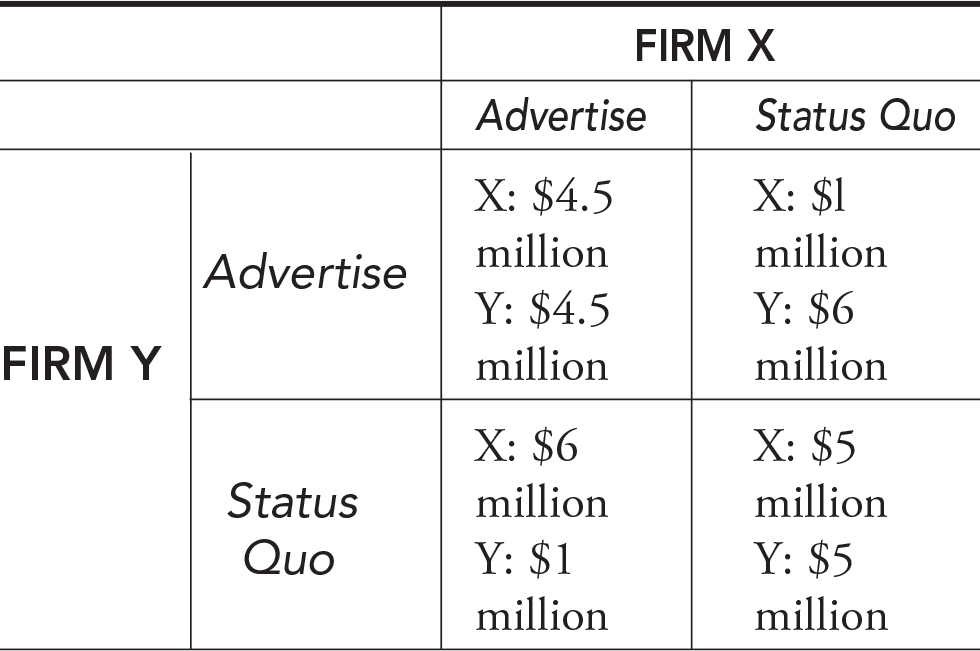
5. If these firms do not collude, the outcome will be that
(A) both firms maintain the status quo.
(B) both firms advertise.
(C) Firm X advertises and Firm Y maintains the status quo.
(D) Firm Y advertises and Firm X maintains the status quo.
(E) Firm X advertises and Firm Y alternates between the status quo and advertising.
6. Deadweight loss occurs in
(A) monopolistic competition as P > MC.
(B) monopoly markets because P > MC.
(C) oligopoly markets because P > MC.
(D) All of the above.
(E) None of the above.
 Answers and Explanations
1. A—The firm only operates if the total revenue is at least as great as total variable cost. On a per-unit basis, the firm must receive a P = MR that is at least as great as AVC. Since firms pay TFC regardless of production, they are not a factor in whether you should shut down. Choices B, C, and E are wrong because TC and ATC include the fixed costs. Choice D is incorrect because it might not be the profitable strategy, but it is irrelevant to the shutdown decision.
2. B—Monopoly has barriers to entry (e.g., patents) and the monopolistic competitive firm does not. Choices A, C, and D are true of monopolistic competition and monopoly.
3. E—With P > ATC, you should recognize that positive economic profits exist. Firms enter and price falls toward the breakeven point, so any mention of exit or rising prices can be eliminated. Entry also increases the market quantity of the good produced.
4. A—If Brent chooses to buy his bread early in the morning rather than in the evening, this is not price discrimination. The other choices describe buying in bulk, redeeming a coupon, or paying a lower price because of the time in which one consumes the good. The nightclub example is price discrimination based upon gender.
5. B—For each firm, choosing the costly advertising campaign is the dominant strategy. This is an example of the prisoner’s dilemma.
6. D—Allocative inefficiency and deadweight loss in any market structure is when P > MC.
 Rapid Review
Perfect competition: The most competitive market structure is characterized by many small price-taking firms producing a standardized product in an industry in which there are no barriers to entry or exit.
Profit maximizing rule: All firms maximize profit by producing where MR = MC.
Breakeven point: The output in perfect competition where ATC is minimized and economic profit is zero.
Shutdown point: The output where AVC is minimized. If the price falls below this point, the firm chooses to shut down or produce zero units in the short run.
Perfectly competitive long-run equilibrium: Occurs when there is no more incentive for firms to enter or exit. P = MR = MC = ATC and π = 0.
Normal profit: Another way of saying that firms are earning zero economic profits or a fair rate of return on invested resources.
Constant cost industry: Entry (or exit) of firms does not shift the cost curves of firms in the industry.
Increasing cost industry: Entry of new firms shifts the cost curves for all firms upward.
Decreasing cost industry: Entry of new firms shifts the cost curves for all firms downward.
Monopoly: The least competitive market structure; it is characterized by a single producer, with no close substitutes, barriers to entry, and price-making power.
Market power: The ability to set the price above the perfectly competitive level.
Natural monopoly: The case where economies of scale are so extensive that it is less costly for one firm to supply the entire range of demand.
Monopoly long-run equilibrium: Pm > MR = MC, which is not allocatively efficient and deadweight loss exists. Pm > ATC, which is not productively efficient. πm > 0 so consumer surplus is transferred to the monopolist as profit.
Price discrimination: The practice of selling essentially the same good to different groups of consumers at different prices.
Perfect price discrimination: The type of price discrimination in which each consumer pays exactly his or her maximum willingness to pay. Consumer surplus is eliminated, yet the allocatively efficient output is produced.
Monopolistic competition: A market structure characterized by a few small firms producing a differentiated product with easy entry into the market.
Monopolistic competition long-run equilibrium: Pmc > MR = MC and Pmc > minimum ATC, so the outcome is not efficient, but πmc = 0.
Excess capacity: The difference between the monopolistic competition output Qmc and the output at minimum ATC. Excess capacity is underused plant and equipment.
Oligopoly: A very diverse market structure characterized by a small number of interdependent large firms, producing a standardized or differentiated product in a market with a barrier to entry.
Four-firm concentration ratio: A measure of industry market power. If the combined market share of the four largest firms is above 40 percent, it is a good indicator of oligopoly.
Noncollusive oligopoly: Models where firms are competitive rivals seeking to gain at the expense of their rivals.
Prisoner’s dilemma: A game where the two rivals achieve a less desirable outcome because they are unable to coordinate their strategies.
Dominant strategy: A strategy that is always the best strategy to pursue, regardless of what a rival is doing.
Nash equilibrium: The outcome of a game for which each player’s strategy maximizes his or her payoff, given the strategies used by the rival players.
Collusive oligopoly: Models where firms agree to mutually improve their situation.
Cartel: A group of firms that agree not to compete with each other on the basis of price, production, or other competitive dimensions. Cartel members operate as a monopolist to maximize their joint profits.