
In these days the angel of topology and the devil of abstract algebra fight for the soul of each individual mathematical domain.
HERMANN WEYL
While non-Euclidean and Riemannian geometry were being created, the projective geometers were pursuing their theme. As we have seen, the two areas were linked by the work of Cayley and Klein. After the algebraic method became widely used in projective geometry the problem of recognizing what properties of geometrical figures are independent of the coordinate representation commanded attention and this prompted the study of algebraic invariants.
The projective properties of geometrical figures are those that are invariant under linear transformations of the figures. While working on these properties the mathematicians occasionally allowed themselves to consider higher-degree transformations and to seek those properties of curves and surfaces that are invariant under these latter transformations. The class of transformations, which soon superseded linear transformations as the favorite interest, is called birational because these are expressed algebraically as rational functions of the coordinates and the inverse transformations are also rational functions of their coordinates. The concentration on birational transformations undoubtedly resulted from the fact that Riemann had used them in his work on Abelian integrals and functions, and in fact, as we shall see, the first big steps in the study of the birational transformation of curves were guided by what Riemann had done. These two subjects formed the content of algebraic geometry in the latter part of the nineteenth century.
The term algebraic geometry is an unfortunate one because originally it referred to all the work from the time of Fermât and Descartes in which algebra had been applied to geometry; in the latter part of the nineteenth century it was applied to the study of algebraic invariants and birational transformations. In the twentieth century it refers to the last-mentioned field.
As we have already noted, the determination of the geometric properties of figures that are represented and studied through coordinate representation calls for the discernment of those algebraic expressions which remain invariant under change of coordinates. Alternatively viewed, the projective transformation of one figure into another by means of a linear transformation preserves some properties of the figure. The algebraic invariants represent these invariant geometrical properties.
The subject of algebraic invariants had previously arisen in number theory (Chap. 34, sec. 5)and particularly in the study of how binary quadratic forms
transform when x and y are transformed by the linear transformation T, namely,

where αδ – βγ = r. Application of T to f produces

In number theory the quantities a, b, c, α, α, γ, and δ are integers and r = 1. However, it is true generally that the discriminant Do if satisfies the relation

The linear transformations of projective geometry are more general because the coefficients of the forms and the transformations are not restricted to integers. The term algebraic invariants is used to distinguish those arising under these more general linear transformations from the modular invariants of number theory and, for that matter, from the differential invariants of Riemannian geometry.
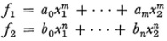
To discuss the history of algebraic invariant theory we need some definitions. The ?ith degree form in one variable
f(x) = a0xn + a1xn +… + an
becomes in homogeneous coordinates the binary form

In three variables the forms are called ternary; in four variables, quaternary; etc. The definitions below apply to forms in n variables.
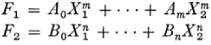
Suppose we subject the binary form to a transformation T of the form (2). Under T the form f(xx, x2)) is transformed into the form
F (X1, X2) = A0Xn1 + A1Xn1 X2 +…+ AnXn1
The coefficients of F will differ from those of ƒ and the roots of F = 0 will differ from the roots of f = 0. Any function I of the coefficients of ƒ which satisfies the relationship
I(A0, A1,…,An)) = rwI(a0, ax,…, an))
is called an invariant of ƒ. If w = 0, the invariant is called an absolute invariant of f. The degree of the invariant is the degree in the coefficients and the weight is w. The discriminant of a binary form is an invariant, as (4) illustrates. In this case the degree is 2 and the weight is 2. The significance of the discriminant of any polynomial equation f(x) =0 is that its vanishing is the condition that f(x) = 0 have equal roots or, geometrically, that the locus of f(x) = 0, which is a series of points, has two coincident points. This property is clearly independent of the coordinate system.
If two (or more) binary forms
are transformed by x into
then any function I of the coefficients which satisfies the relationship

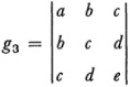
is said to be a joint or simultaneous invariant of the two forms. Thus the linear forms a1x1 + b1x2 and a2x1 + b2x2 have as a simultaneous invariant the resultant a1x1 +b1x2 — a 2 b bx of the two forms. Geometrically the vanishing of the resultant means that the two forms represent the same point (in homogeneous coordinates). Two quadratic forms f1 = a1x21 + 2b1x12 + c1x22 and f2 = a2x21 + 2b2x1x2 + c2x22
D12 = a1 c 2 – 2b1b2 + a2c1
whose vanishing expresses the fact that f1 and f2 represent harmonic pairs of points.
Beyond invariants of a form or system of forms there are covariants. Any function C of the coefficients and variables of f which is an invariant under T except for a power of the modulus (determinant) of T is called a covariant of f. Thus, for binary forms, a covariant satisfies the relation
C(A0, A1,…, An, X1, X2)) — rwC(a0, a1,…, an, x1, x2)
The definitions of absolute and simultaneous covariants are analogous to those for invariants. The degree of a covariant in the coefficients is called its degree and the degree in its variables is called its order. Invariants are thus covariants of order zero. However, sometimes the word invariant is used to mean an invariant in the narrower sense or a covariant.
covariants of order zero. However, sometimes the word invariant is used to mean an invariant in the narrower sense or a covariant.
A covariant of f ” represents some figure which is not only related to ƒ but projectively related. Thus the Jacobian of two quadratic binary forms f (x1, x2) and φ (x1,x2), namely,
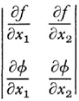
is a simultaneous covariant of weight 1 of the two forms. Geometrically, the Jacobian set equal to zero represents a pair of points which is harmonic to each of the original pairs represented by ƒ and Φ and the harmonic property is projective.
The Hessian of a binary form introduced by Hesse,1
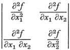
is a covariant of weight 2. Its geometric meaning is too involved to warrant space here (Cf. Chap. 35, sec. 5). The concept of the Hessian and its covariance applies to any form in n variables.
The work on algebraic invariants was started in 1841 by George Boole (1815-64) whose results2 were limited. What is more relevant is that Cayley was attracted to the subject by Boole’s work and he interested Sylvester in the subject. They were joined by George Salmon (1819-1904), who was a professor of mathematics at Trinity College in Dublin from 1840 to 1866 and then became a professor of divinity at that institution. These three men did so much work on invariants that in one of his letters Hermite dubbed them the invariant trinity.
In 1841 Cayley began to publish mathematical articles on the algebraic side of projective geometry. The 1841 paper of Boole suggested to Cayley the computation of invariants of nth degree homogeneous functions. He called the invariants derivatives and then hyperdeterminants; the term invariant is due to Sylvester.3 Cayley, employing ideas of Hesse and Eisenstein on determinants, developed a technique for generating his “derivatives.” Then he published ten papers on quantics in the Philosophical Transactions from 1854
to 1878.4 Quantics was the term he adopted for homogeneous polynomials in 2, 3, or more variables. Cayley became so much interested in invariants that he investigated them for their own sake. He also invented a symbolic method of treating invariants.
In the particular case of the binary quartic form

Cayley showed that the Hessian H and the Jacobian of f and H are covariants and that
g2 = ae – 4bd + 3c2
and
are invariants. To these results Sylvester and Salmon added many more.
Another contributor, Ferdinand Eisenstein, who was more concerned with the theory of numbers, had already found for the binary cubic form5

that the simplest covariant of the second degree is its Hessian H and the simplest invariant is

which is the determinant of the quadratic Hessian as well as the discriminant of ƒ. Also the Jacobian of ƒ and H is another covariant of order three. Then Siegfried Heinrich Aronhold (1819-84), who began work on invariants in 1849, contributed invariants for ternary cubic forms.6
The first major problem that confronted the founders of invariant theory was the discovery of particular invariants. This was the direction of the work from about 1840 to 1870. As we can see, many such functions can be constructed because some invariants such as the Jacobian and the Hessian are themselves forms that have invariants and because some invariants taken together with the original form give a new system of forms that have simultaneous invariants. Dozens of major mathematicians including the few we have already mentioned computed particular invariants.
The continued calculation of invariants led to the major problem of invariant theory, which was raised after many special or particular invariants were found; this was to find a complete system of invariants. What
this means is to find for a form of a given number of variables and degree the smallest possible number of rational integral invariants and covariants such that any other rational integral invariant or covariant could be expressed as a rational integral function with numerical coefficients of this complete set. Cayley showed that the invariants and covariants found by Eisenstein for the binary cubic form and the ones he obtained for the binary quartic form are a complete system for the respective cases.7 This left open the question of a complete system for other forms.
The existence of a finite complete system or basis for binary forms of any given degree was first established by Paul Gordan (1837-1912), who devoted most of his life to the subject. His result8 is that to each binary form f(xu X2Ì there belongs a finite complete system of rational integral invariants and covariants. Gordan had the aid of theorems due to Clebsch and the result is known as the Clebsch-Gordan theorem. The proof is long and difficult. Gordan also proved 9 that any finite system of binary forms has a finite complete system of invariants and covariants. Gordan’s proofs showed how to compute the complete systems.
Various limited extensions of Gordan’s results were obtained during the next twenty years. Gordan himself gave the complete system for the ternary quadratic form,10 for the ternary cubic form,11 and for a system of two and three ternary quadratics.12 For the special ternary quartic x31 + x31 + x33 + x1 Gordan gave a complete system of 54 ground forms.13
In 1886 Franz Mertens (1840-1927)14 re-proved Gordan’s theorem for binary systems by an inductive method. He assumed the theorem to be true for any given set of binary forms and then proved it must still be true when the degree of one of the forms is increased by one. He did not exhibit explicitly the finite set of independent invariants and covariants but he proved that it existed. The simplest case, a linear form, was the starting point of the induction and such a form has only powers of itself as covariants.
Hilbert, after writing a doctoral thesis in 1885 on invariants,15 in 188816also re-proved Gordan’s theorem that any given system of binary forms has a finite complete system of invariants and covariants. His proof was a modification of Mertens’s. Both proofs were far simpler than Gordan’s. But Hubert’s proof also did not present a process for finding the complete system.
In 1888 Hilbert astonished the mathematical community by announcing a totally new approach to the problem of showing that any form of given degree and given number of variables, and any given system of forms in any given number of variables, have a finite complete system of independent rational integral invariants and covariante.17 The basic idea of this new approach was to forget about invariants for the moment and consider the question: If an infinite system of rational integral expressions in a finite number of variables be given, under what conditions does a finite number of these expressions, a basis, exist in terms of which all the others are expressible as linear combinations with rational integral functions of the same variables as coefficients ? The answer is, Always. More specifically, Hubert’s basis theorem, which precedes the result on invariants, goes as follows: By an algebraic form we understand a rational integral homogeneous function in x variables with coefficients in some definite domain of rationality (field). Given a collection of infinitely many forms of any degrees in the n variables, then there is a finite number (a basis) F1, F2, …, Fm such that any form F of the collection can be written as
F = A1F1 + A2F2 +… +AmFm
where A1 A2, …, Am are suitable forms in the x variables (not necessarily in the infinite system) with coefficients in the same domain as the coefficients of the infinite system.
In the application of this theorem to invariants and covariants, Hubert’s result states that for any form or system of forms there is a finite number of rational integral invariants and covariants by means of which every other rational integral invariant or covariant can be expressed as a linear combination of the ones in the finite set. This finite collection of invariants and covariants is the complete invariant system.
Hilbert’s existence proof was so much simpler than Gordan’s laborious calculation of a basis that Gordan could not help exclaiming, “This is not mathematics; it is theology.” However, he reconsidered the matter and said later, “I have convinced myself that theology also has its advantages.” In fact he himself simplified Hubert’s existence proof.18
In the 1880s and '90s the theory of invariants was seen to have unified many areas of mathematics. This theory was the “modern algebra” of the period. Sylvester said in 1864:19 “As all roads lead to Rome so I find in my own case at least that all algebraic inquiries, sooner or later, end at the Capitol of modern algebra over whose shining portal is inscribed the Theory of Invariants.” Soon the theory became an end in itself, independent of its origins in number theory and projective geometry. The workers in algebraic invariants persisted in proving every kind of algebraic identity whether or not it had geometrical significance. Maxwell, when a student at Cambridge, said that some of the men there saw the whole universe in terms of quintics and quantics.
On the other hand the physicists of the late nineteenth century took no notice of the subject. Indeed Tait once remarked of Cayley, “Is it not a shame that such an outstanding man puts his abilities to such entirely useless questions?” Nevertheless the subject did make its impact on physics, indirectly and directly, largely through the work in differential invariants.
Despite the enormous enthusiasm for invariant theory in the second half of the nineteenth century, the subject as conceived and pursued during that period lost its attraction. Mathematicians say Hilbert killed invariant theory because he had disposed of all the problems. Hilbert did write to Minkowski in 1893 that he would no longer work in the subject, and said in a paper of 1893 that the most important general goals of the theory were attained. However, this was far from the case. Hubert’s theorem did not show how to compute invariants for any given form or system of forms and so could not provide a single significant invariant. The search for specific invariants having geometrical or physical significance was still important. Even the calculation of a basis for forms of a given degree and number of variables might prove valuable.
What “killed” invariant theory in the nineteenth-century sense of the subject is the usual collection of factors that killed many other activities that were over-enthusiastically pursued. Mathematicians follow leaders. Hubert’s pronouncement, and the fact that he himself abandoned the subject, exerted great influence on others. Also, the calculation of significant specific invariants had become more difficult after the more readily attainable results were achieved.
The computation of algebraic invariants did not end with Hilbert’s work. Emmy Noether (1882-1935), a student of Gordan, did a doctoral thesis in 1907 “On Complete Systems of Invariants for Ternary Biquadratic Forms.”20She also gave a complete system of covariant forms for a ternary quartic, 331 in all. In 1910 she extended Gordan’s result to x variables.21
The subsequent history of algebraic invariant theory belongs to modern abstract algebra. The methodology of Hilbert brought to the fore the abstract theory of modules, rings, and fields. In this language Hilbert proved that every modular system (an ideal in the class of polynomials in x variables) has a basis consisting of a finite number of polynomials, or every ideal in a polynomial domain of « variables possesses a finite basis provided that in the domain of the coefficients of the polynomials every ideal has a finite basis. From 1911 to 1919 Emmy Noether produced many papers on finite bases for various cases using Hubert’s technique and her own. In the subsequent twentieth-century development the abstract algebraic viewpoint dominated. As Eduard Study complained in his text on invariant theory, there was lack of concern for specific problems and only abstract methods were pursued.
We saw in Chapter 35 that, especially during the third and fourth decades of the nineteenth century, the work in projective geometry turned to higher-degree curves. However, before this work had gone very far there was a change in the nature of the study. The projective viewpoint means linear transformations in homogeneous coordinates. Gradually transformations of the second and higher degrees came into play and the emphasis turned to birational transformations. Such a transformation, for the case of two non-homogeneous coordinates, is of the form
x′ = Φ (x, y), y′ = ψ(x, y)
where Φ and ψ are rational functions in x and y and moreover x and y can be expressed as rational functions of x’ and y’. In homogeneous coordinates x1, x2, x3 the transformation are of the form
and the inverse is

where Fi and Gi are homogeneous polynomials of degree p in their respective variables. The correspondence is one-to-one except that each of a finite number of points may correspond to a curve.
As an illustration of a birational transformation we have inversion with respect to a circle. Geometrically this transformation (Fig. 39.1) is from M to M’ or M’ to M by means of the defining equation
OM · OM′ = r2,
where r is the radius of the circle. Algebraically if we set up a coordinate system at 0 the Pythagorean theorem leads to
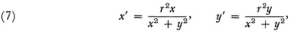
where M is (x, y) and M′ is (x′, y′). Under this transformation circles transform into circles or straight lines and conversely. Inversion is a transformation that carries the entire plane into itself and such birational transformations
are called Cremona transformations. Another example of a Cremona transformation in three (homogeneous) variables is the quadratic transformation

whose inverse is

The term birational transformation is also used in a more general sense, namely, wherein the transformation from the points of one curve into those of another is birational but the transformation need not be birational in the entire plane. Thus (in nonhomogeneous coordinates) the transformation

is not one-to-one in the entire plane but does take any curve C to the right of the y-axis into another in a one-to-one correspondence.
The inversion transformation was the first of the birational transformations to appear. It was used in limited situations by Poncelet in his Traité of 1822 (11370) and then by Plücker, Steiner, Quetelet, and Ludwig Immanuel Magnus (1790-1861). It was studied extensively by Möbius22and its use in physics was recognized by Lord Kelvin,23 and by Liouville,24who called it the transformation by reciprocal radii.
In 1854 Luigi Cremona (1830-1903), who served as a professor of mathematics at several Italian universities, introduced the general birational transformation (of the entire plane into itself) and wrote important papers on it.25 Max Noether (1844-1921), the father of Emmy Noether, then proved the fundamental result26 that a plane Cremona transformation can be built up from a sequence of quadratic and linear transformations. Jacob Rosanes (1842-1922) found this result independently27 and also proved that all one-to-one algebraic transformations of the plane must be Cremona transformations. The proofs of Noether and Rosanes were completed by Guido Castelnuovo (1865-1952).28
Though the nature of the birational transformation was clear, the development of the subject of algebraic geometry as the study of invariants under such transformations was, at least in the nineteenth century, unsatisfactory. Several approaches were used; the results were disconnected and fragmentary; most proofs were incomplete; and very few major theorems were obtained. The variety of approaches has resulted in marked differences in the languages used. The goals of the subject were also vague. Though invariance under birational transformations has been the leading theme, the subject covers the search for properties of curves, surfaces, and higher-dimensional structures. In view of these factors there are not many central results. We shall give a few samples of what was done.
The first of the approaches was made by Clebsch. (Rudolf Friedrich) Alfred Clebsch (1833-72) studied under Hesse in Königsberg from 1850 to 1854. In his early work he was interested in mathematical physics and from 1858 to 1863 was professor of theoretical mechanics at Karlsruhe and then professor of mathematics at Giessin and Göttingen. He worked on problems left by Jacobi in the calculus of variations and the theory of differential equations. In 1862 he published the Lehrbuch der Elasticität. However, his chief work was in algebraic invariants and algebraic geometry.
Clebsch had worked on the projective properties of curves and surfaces of third and fourth degrees up to about 1860. He met Paul Gordan in 1863 and learned about Riemann’s work in complex function theory. Clebsch then brought this theory to bear on the theory of curves.29 This approach is called transcendental. Though Clebsch made the connection between complex functions and algebraic curves, he admitted in a letter to Gustav Roch that he could not understand Riemann’s work on Abelian functions nor Roch’s contributions in his dissertation.
Clebsch reinterpreted the complex function theory in the following manner: The function f(w, z) = 0, wherein ?and w are complex variables, calls geometrically for a Riemann surface for ?and a plane or a portion of a plane for w or, if one prefers, for a Riemann surface to each point of which a pair of values of ?and w is attached. By considering only the real parts of ?
and w the equation f(w, z) = 0 represents a curve in the real Cartesian plane, z and w may still have complex values satisfying ƒ (w, z) = 0 but these are not plotted. This view of real curves with complex points was already familiar from the work in projective geometry. To the theory of birational transformations of the surface corresponds a theory of birational transformations of the plane curve. Under the reinterpretation just described the branch points of the Riemann surface correspond to those points of the curve where a line x = const, meets the curve in two or more consecutive points, that is, is either tangent to the curve or passes through a cusp. A double point of the curve corresponds to a point on the surface where two sheets just touch without any further connection. Higher multiple points on curves also correspond to other peculiarities of Riemann surfaces.
In the subsequent account we shall utilize the following definitions (Cf. Chap. 23, sec. 3): A multiple point (singular point) P of order k > 1 of an nth degree plane curve is a point such that a generic line through P cuts the curve in n — k points. The multiple point is ordinary if the P tangents at P are distinct. In counting intersections of an nth degree and an mth degree curve one must take into account the multiplicity of the multiple points on each curve. If it is h on the curve Cn and c on Cm and if the tangents at x of Cn are distinct from those of Cm, then the point of intersection has multiplicity hk. A curve C' is said to be adjoint to a curve p when the multiple points of p are ordinary or cusps and if C' has a point of multiplicity of order k — 1 at every multiple point of C of order k.
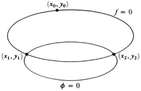
Clebsch30 first restated Abel’s theorem (Chap. 27, sec. 7) on integrals of the first kind in terms of curves. Abel considered a fixed rational function R{x, y) where x and y are related by any algebraic curve f(x, y) = 0, so that y is a function of x. Suppose (Fig. 39.2) ƒ = 0 is cut by another algebraic curve
Φ(x, y, a1, a2,, …, ak) = 0
where the ai’s are the coefficients in Φ = 0. Let the intersections of Φ = 0 with ƒ = 0 be (x1, y1), (x2, y2), (x2, y2),…, (xm, ym). (The number m of these is the
product of the degrees of f and Φ.) Given a point (x0, y0) on f = 0, where y0 belongs to one branch of f = 0, then we can consider the sum
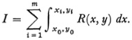
The upper limits xi, yi all lie on Φ = 0 and the integral I is a function of the upper limits. Then there is a characteristic number p of these limits which have to be algebraic functions of the others. This number p depends only on ƒ. Moreover. I can be expressed as the sum of these p integrals and rational and logarithmic functions of the xi, yi, i = 1, 2, …, m. Further, if the curve Φ = 0 is varied by varying the parameters a1 to ak then the xi will also vary and I becomes a function of the a1 through the x1. The function I of the ai will be rational in the ai or at worst involve logarithmic functions of the ai.
Clebsch also carried over to curves Riemann’s concept of Abelian integrals on Riemann surfaces, that is, integrals of the form ƒ g(x, y) dx, where g is a rational function and f{x, y) = 0. To illustrate the integrals of the first kind consider a plane fourth degree curve C4 without double points. Here p = 3 and there are the three everywhere finite integrals
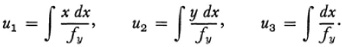
What applies to the C4 carries over to arbitrary algebraic curves f(x, y) = 0 of the nth order. In place of the three everywhere finite integrals there are now ƒ such integrals, (where p is the genus of f = 0). Each has 2p periodicity modules (Chap. 27, sec. 8). The integrals are of the form

where Φ is a polynomial (an adjoint) of precisely the degree n — 3 which vanishes at the double points and cusps of f = 0.
Clebsch’s next contribution31 was to introduce the notion of genus as a concept for classifying curves. If the curve has d double points then the genus p = (l/2)(n — l)(n — 2) — d. Previously there was the notion of the deficiency of a curve (Chap. 23, sec. 3), that is, the maximum possible number of double points a curve of degree x could possess, namely, (n — l)(n — 2)/2, minus the number it actually does possess. Clebsch showed32 that for curves with only ordinary multiple points (the tangents are all distinct) the genus is the same as the deficiency and the genus is an invariant under birational transformation of the entire plane into itself.33
Clebsch’s notion of genus is related to Riemann’s connectivity of a Riemann surface. The Riemann surface corresponding to a curve of genus p has connectivity 2p + 1.
The notion of genus can be used to establish significant theorems about curves. Jacob Lüroth (1844-1910) showed34 that a curve of genus 0 can be birationally transformed into a straight line. When the genus is 1, Clebsch showed that a curve can be birationally transformed into a third degree curve.
In addition to classifying curves by genus, Clebsch, following Riemann, introduced classes within each genus. Riemann had considered35 the birational transformation of his surfaces. Thus iif(w, z) = 0 is the equation of the surface and if
w1 = R1(w, z), z1 = R2(w, z)
are rational functions and if the inverse transformation is rational then f(w, z) can be transformed to F(w1, , zf) — 0. Two algebraic equations F(w, z) = 0 (or their surfaces) can be transformed birationally into one another only if both have the same p value. (The number of sheets need not be preserved.) For Riemann no further proof was needed. It was guaranteed by the intuition.
Riemann (in the 1857 paper) regarded all equations (or the surfaces) which are birationally transformable into each other as belonging to the same class. They have the same genus p. However, there are different classes with the same p value (because the branch-points may differ). The most general class of genus p is characterized by 3p — 3 (complex) constants (coefficients in the equation) when p < 1, by one constant when p = 1 and by zero constants when jö = 0. In the case of elliptic functions/) = 1 and there is one constant. The trigonometric functions, for which p = 0, do not have any arbitrary constant. The number of constants was called by Riemann the class modulus. The constants are invariant under birational transformation. Clebsch likewise put all those curves which are derivable from a given one by a one-to-one birational transformation into one class. Those of one class necessarily have the same genus but there may be different classes with the same genus.
Clebsch then turned his attention to what is called the uniformization problem for curves. Let us note first just what this problem amounts to. Given the equation

we can represent it in the parametric form

or in the parametric form
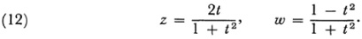
Thus even though (10) defines it) as a multiple-valued function of z, we can represent ?and w as single-valued or uniform functions of t. The parametric equations (11) or (12) are said to uniformize the algebraic equation (10).
For an equation f(w, z)= 0 of genus 0 Clebsch36 showed that each of the variables can be expressed as a rational function of a single parameter. These rational functions are uniformizing functions. When ƒ = 0 is interpreted as a curve it is then called unicursal. Conversely if the variables w and z of f = 0 are rationally expressible in terms of an arbitrary parameter then f = 0 is of genus 0.
When p = 1 then Clebsch showed in the same year37 that w and ?can be expressed as rational functions of the parameters ξ and n where n2 is a polynomial of either the third or fourth degree in ξ. Then f (w, z)= 0 or the corresponding curve is called bicursal, a term introduced by Cayley.38 It is also called elliptic because the equation (dwjdz)2 = n2 leads to elliptic integrals. We can as well say that w and ?are expressible as single-valued doubly periodic functions of a single parameter ? or as rational functions of p (α) where p(α) is Weierstrass’s function. Clebsch’s result on the uniformiza-tion of curves of genus 1 by means of elliptic functions of a parameter made it possible to establish for such curves remarkable properties about points of inflection, osculatory conies, tangents from a point to a curve, and other results, many of which had been demonstrated earlier but with great difficulty.
For equations f(w, z)= 0 of genus 2, Alexander von Brill (1842-1935) showed39 that the variables w and ?are expressible as rational functions of x and y where 12 is now a polynomial of the fifth or sixth degree in ξ.
Thus functions of genus 0, 1, and 2 can be uniformized. For function ƒ (if, z)= 0 of genus greater than 2 the thought was to employ more general functions, namely, automorphic functions. In 1882 Klein40 gave a general uniformization theorem but the proof was not complete. In 1883 Poincaré announced41 his general uniformization theorem but he too had no complete
proof. Both Klein and Poincaré continued to work hard to prove this theorem but no decisive result was obtained for twenty-five years. In 1907 Poincaré42 and Paul Koebe (1882-1945)43 independently gave a proof of this uniformization theorem. Koebe then extended the result in many directions. With the theorem on uniformization now rigorously established an improved treatment of algebraic functions and their integrals has become possible.
A new direction of work in algebraic geometry begins with the collaboration of Clebsch and Gordan during the years 1865-70. Clebsch was not satisfied merely to show the significance of Riemann’s work for curves. He sought now to establish the theory of Abelian integrals on the basis of the algebraic theory of curves. In 1865 he and Gordan joined forces in this work and produced their Theorie der Abelschen Funktionen (1866). One must appreciate that at this time Weierstrass’s more rigorous theory of Abelian integrals was not known and Riemann’s foundation—his proof of existence based on Dirichlet’s principle—was not only strange but not well established. Also at this time there was considerable enthusiasm for the theory of invariants of algebraic forms (or curves) and for projective methods as the first stage, so to speak, of the treatment of birational transformations.
Although the work of Clebsch and Gordan was a contribution to algebraic geometry, it did not establish a purely algebraic theory of Riemann’s theory of Abelian integrals. They did use algebraic and geometric methods as opposed to Riemann’s function-theoretic methods but they also used basic results of function theory and the function-theoretic methods of Weierstrass. In addition they took some results about rational functions and the intersection point theorem as given. Their contribution amounted to starting from some function-theoretic results and, using algebraic methods, obtaining new results previously established by function-theoretic methods. Rational transformations were the essence of the algebraic method.
They gave the first algebraic proof for the invariance of the genus p of an algebraic curve under rational transformations, using as a definition of p the degree and number of singularities of f = 0. Then, using the fact that p is the number of linearly independent integrals of the first kind on ƒ(x1, x2 x3) — 0 and that these integrals are everywhere finite, they showed that the transformation
pXi = φ1 ((y1, y2, y3), i = 1, 2, 3,
transforms an integral of the first kind into an integral of the first kind so that p is invariant. They also gave new proofs of Abel’s theorem (by using function-theoretic ideas and methods).
Their work was not rigorous. In particular they, too, in the Plücker tradition counted arbitrary constants to determine the number of intersection points of a Cm with a Cn. Special kinds of double points were not investigated. The significance of the Glebsch-Gordan work for the theory of algebraic functions was to express clearly in algebraic form such results as Abel’s theorem and to use it in the study of Abelian integrals. They put the algebraic part of the theory of Abelian integrals and functions more into the foreground and in particular established the theory of transformations on its own foundations.
Clebsch and Gordan had raised many problems and left many gaps. The problems lay in the direction of new algebraic investigations for a purely algebraic theory of algebraic functions. The work on the algebraic approach was continued by Alexander von Brill and Max Noether from 1871on; their key paper was published in 1874.44 Brill and Noether based their theory on a celebrated residual theorem (Restsatz) which in their hands took the place of Abel’s theorem. They also gave an algebraic proof of the Riemann-Roch theorem on the number of constants which appear in algebraic functions F(w, z) which become infinite nowhere except in m prescribed points of a Cn. According to this theorem the most general algebraic function which fulfills this condition has the form
F = C1F1 + C2F2 +… + Cμ+1
where
μ = m — p +r,
τ is the number of linearly independent functions φ (of degree n — 3)which vanish in the m prescribed points, and p is the genus of the Cn. Thus if the Cn i is a C4 without double points, then p = 3and the λ are straight lines. For this case when
m = 1, then τ = 2 and μ=1 – 3 + 2 = 0;
m = 2, then τ = 1, and μ = 2 – 3 + 1 = 0;
m = 3, then τ = 1 or 0and μ = 1 or 0.
When μ = 0there is no algebraic function which becomes infinite in the given points. When m = 3, there is one and only one such function provided the three given points be on a straight line. If the three points do lie on a line x = 0, this line cuts the C4 in a fourth point. We choose a line y = 0through this point and then Fx = u/v.
This work replaces Riemann’s determination of the most general algebraic function having given points at which it becomes infinite. Also the Brill-Noether result transcends the projective viewpoint in that it deals with the geometry of points on the curve Cn given by ƒ = 0, whose mutual relations are not altered by a one-to-one birational transformation. Thus for the first time the theorems on points of intersection of curves were established algebraically. The counting of constants as a method was dispensed with.
The work in algebraic geometry continued with the detailed investigation of algebraic space curves by Noether45 and Halphen.46 Any space curve x can be projected birationally into a plane curve Cx. All such Cx c coming from a have the same genus. The genus of p is therefore defined to be that of any such Cx and the genus of p is invariant under birational transformation of the space.
The topic which has received the greatest attention over the years is the study of singularities of plane algebraic curves. Up to 1871, the theory of algebraic functions considered from the algebraic viewpoint had limited itself to curves which had distinct or separated double points and at worst only cusps (Rückkehrpunkte). Curves with more complicated singularities were believed to be treatable as limiting cases of curves with double points. But the actual limiting procedure was vague and lacked rigor and unity. The culmination of the work on singularities is two famous transformation theorems. The first states that every plane irreducible algebraic curve can be transformed by a Cremona transformation to one having no singular points other than multiple points with distinct tangents. The second asserts that by a transformation birational only on the curve every plane irreducible algebraic curve can be transformed into another having only double points with distinct tangents. The reduction of curves to these simpler forms facilitates the application of many of the methodologies of algebraic geometry.
However, the numerous proofs of these theorems, especially the second one, have been incomplete or at least criticized by mathematicians (other than the author). There really are two cases of the second theorem, real curves in the projective plane and curves in the complex function theory sense where x and y each run over a complex plane. Noether47 in 1871 used a sequence of quadratic transformations which are one-to-one in the entire plane to prove the first theorem. He is generally credited with the proof but actually he merely indicated a proof which was perfected and modified by many writers.48 Kronecker, using analysis and algebra, developed a method for proving the second theorem. He communicated this method verbally to
Riemann and Weierstrass in 1858, lectured on it from 1870 on and published it in 1881.49 The method used rational transformations, which with the aid of the equation of the given plane curve are one-to-one, and transformed the singular case into the “regular one;” that is, the singular points become just double points with distinct tangents. The result, however, was not stated by Kronecker and is only implicit in his work.
This second theorem to the effect that all multiple points can be reduced to double points by birational transformations on the curve was first explicitly stated and proved by Halphen in 1884.50 Many other proofs have been given but none is universally accepted.
In addition to the transcendental approach and the algebraic-geometric approach there is what is called the arithmetic approach to algebraic curves, which is, however, in concept at least, purely algebraic. This approach is really a group of theories which differ greatly in detail but which have in common the construction and analysis of the integrands of the three kinds of Abelian integrals. This approach was developed by Kronecker in his lectures,51 by Weierstrass in his lectures of 1875-76, and by Dedekind and Heinrich Weber in a joint paper.52 The approach is fully presented in the text by Kurt Hensel and Georg Landsberg: Theorie der algebraischen Funktionen einer Variabein (1902).
The central idea of this approach comes from the work on algebraic numbers by Kronecker and Dedekind and utilizes an analogy between the algebraic integers of an algebraic number field and the algebraic functions on the Riemann surface of a complex function. In the theory of algebraic numbers one starts with an irreducible polynomial equation f(x) =0 with integral coefficients. The analogue for algebraic geometry is an irreducible polynomial equation ƒ(ζ, z) = 0 whose coefficients of the powers of ζ are polynomials in z (with, say, real coefficients). In number theory one then considers the field R(x) generated by the coefficients of f(x) = 0 and one of its roots. In the geometry one considers the field of all R(ζ, z) which are algebraic and one-valued on the Riemann surface. One then considers in the number theory the integral algebraic numbers. To these there correspond the algebraic functions G(ζ, z)which are entire, that is, become infinite only at z= ∞. The decomposition of the algebraic integers into real prime factors
and units respectively corresponds to the decomposition of the G(£, z) into factors such that each vanishes at one point only of the Riemann surface and factors that vanish nowhere, respectively. Where Dedekind introduced ideals in the number theory to discuss divisibility, in the geometric analogue one replaces a factor of a G(£, z) which vanishes at one point of the Riemann surface by the collection of all functions of the field of x(y, z) which vanish at that point. Dedekind and Weber used this arithmetic method to treat the field of algebraic functions and they obtained the classic results.
Hilbert53 continued what is essentially the algebraic or arithmetic approach to algebraic geometry of Dedekind and Kronecker. One principal theorem, Hubert’s Nullstellensatz, states that every algebraic structure (figure) of arbitrary extent in a space of arbitrarily many homogeneous variables xu …, x n can always be represented by a finite number of homogeneous equations
F1 = 0,F2 = 0, …,Fμ = 0
so that the equation of any other structure containing the original one can be represented by
M1 F1 +… + Mμ Fμ = 0,
where the M’s are arbitrary homogeneous integral forms whose degree must be so chosen that the left side of the equation is itself homogeneous.
Hilbert following Dedekind called the collection of the a module (the term is now ideal and module now is something more general). One can state Hubert’s result thus: Every algebraic structure of R„ determines the vanishing of a finite module.
Almost from the beginning of work in the algebraic geometry of curves, the theory of surfaces was also investigated. Here too the direction of the work turned to invariants under linear and birational transformations. Like the equation f(x, y) = 0, the polynomial equation f(x, y, z) = 0 has a double interpretation. If x, y, and z take on real values then the equation represents a two-dimensional surface in three-dimensional space. If, however, these variables take on complex values, then the equation represents a four-dimensional manifold in a six-dimensional space.
The approach to the algebraic geometry of surfaces paralleled that for curves. Clebsch employed function-theoretic methods and introduced54
double integrals which play the role of Abelian integrals in the theory of curves. Clebsch noted that for an algebraic surface f(x, y, z) = 0 of degree m with isolated multiple points and ordinary multiple lines, certain surfaces of degree m — 4 ought to play the role which the adjoint curves of degree m — 3 play with respect to a curve of degree m. Given a rational function R(x, y, z) where x, y, and ? are related by f(x, y, z) = 0, if one seeks the double integrals
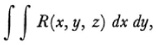
which always remain finite when the integrals extend over a two-dimensional region of the four-dimensional surface, one finds that they are of the form
where Q is a polynomial of degree m — 4. Q = 0 is an adjoint surface which passes through the multiple lines of ƒ = 0 and has a multiple line of order k — 1 at least in every multiple line of ƒ of order k and has a multiple point of order q — 2 at least in every isolated multiple point of ƒ of order q. Such an integral is called a double integral of the first kind. The number of linearly independent integrals of this class, which is the number of essential constants in Q(x, y, z), is called the geometrical genus pg of f = 0. If the surface has no multiple lines of points
Max Noether55 and Hieronymus G. Zeuthen (1839-1920) 56 proved that pg iis an invariant under birational transformations of the surface (not of the whole space).
Up to this point the analogy with the theory of curves is good. The double integrals of the first kind are analogous to the Abelian integrals of the first kind. But now a first difference becomes manifest. It is necessary to calculate the number of essential constants in the polynomials Q of degree m — 4 which behave at multiple points of the surface in such a manner that the integral remains finite. But one can find by a precise formula the number of conditions thus involved only for a polynomial of sufficiently large degree N If one puts into this formula N = m — 4, one might find a number different from pg. Cayley57 called this new number the numerical (arithmetic) genuspn of the surface. The most general case is wherepn = p g. When the equality does not hold one has pn < po and the surface is called irregular; otherwise it is called regular. Then Zeuthen58 and Noether59 established the invariance of the number pn when it is not equal to po
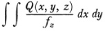
Picard60 developed a theory of double integrals of the second kind. These are the integrals which become infinite in the manner of
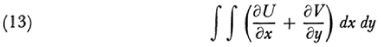
where U and V are rational functions of x, y, and z and f(x, y, z) = 0. The number of different integrals of the second kind, different in the sense that no linear combination of these integrals reduces to the form (13), is finite; this is a birational invariant of the surface f = 0. But it is not true here, as in the case of curves, that the number of distinct Abelian integrals of the second kind is 2p. This new invariant of algebraic surfaces does not appear to be tied to the numerical or the geometrical genus.
Far less has been accomplished for the theory of surfaces than for curves. One reason is that the possible singularities of surfaces are much more complicated. There is the theorem of Picard and Georges Simart proven by Beppo Levi (1875-1928)61 that any (real) algebraic surface can be birationally transformed into a surface free of singularities which must, however, be in a space of five dimensions. But this theorem does not prove to be too helpful.
In the case of curves the single invariant number, the genus/), is capable of definition in terms of the characteristics of the curve or the connectivity of the Riemann surface. In the case of f(x, y, z) = 0 the number of characterizing arithmetical birational invariants is unknown.62 We shall not attempt to describe further the few limited results for the algebraic geometry of surfaces.
The subject of algebraic geometry now embraces the study of higherdimensional figures (manifolds or varieties) defined by one or more algebraic equations. Beyond generalization in this direction, another type, namely, the use of more general coefficients in the defining equations, has also been undertaken. These coefficients can be members of an abstract ring or field and the methods of abstract algebra are applied. The several methods of pursuing algebraic geometry as well as the abstract algebraic formulation introduced in the twentieth century have led to sharp differences in language and methods of approach so that one class of workers finds it very difficult to understand another. The emphasis in this century has been on the abstract algebraic approach. It does seem to offer sharp formulations of theorems and
proofs thereby settling much controversy about the meaning and correctness of the older results. However, much of the work seems to have far more bearing on algebra than on geometry.
Baker, H. F.: “On Some Recent Advances in the Theory of Algebraic Surfaces,” Proc. Lon. Math. Soc, (2), 12, 1912-13, 1-40.
Berzolari, L.: “Allgemeine Theorie der höheren ebenen algebraischen Kurven,” Encyk. der Math. Wiss., ?. G. Teubner, 1903-15, III C4, 313-455.
———: “Algebraische Transformationen und Korrespondenzen,” Encyk. der Math. Wiss., ?. G. Teubner, 1903-15, III, 2, 2nd half B, 1781-2218. Useful for results on higher-dimensional figures.
Bliss, G. A.: “The Reduction of Singularities of Plane Curves by Birational Transformations,” Amer. Math. Soc. Bull, 29, 1923, 161-83.
Brill, A., and M. Noether: “Die Entwicklung der Theorie der algebraischen Funktionen,” Jahres, der Deut. Math.-Verein., 3, 1892-93, 107-565.
Castelnuovo, G., and F. Enriques: “ Die algebraischen Flächen vom Gesichtspunkte der birationalen Transformationen,” Encyk. der Math. Wiss., B. G. Teubner, 1903-15, III C6b, 674-768.
———: “Sur quelques récents résultats dans Ia théorie des surfaces algébriques,” Math. Ann., 48, 1897, 241-316.
Cayley, A.: Collected Mathematical Papers, Johnson Reprint Corp., 1963, Vols. 2, 4, 6, 7, 10, 1891-96.
Clebsch, R. F. ?.: “Versuch einer Darlegung und Würdigung seiner Wissenschaftlichen Leistungen,” Math. Ann., 7, 1874, 1-55. An article by friends of Clebsch.
Coolidge, Julian L.: A History of Geometrical Methods, Dover (reprint), 1963, pp. 195-230, 278-92.
Cremona, Luigi: Opere mathematiche, 3 vols., Ulrico Hoepli, 1914-17.
Hensel, Kurt, and Georg Landsberg: Theorie der algebraischen Funktionen einer Variabein (1902), Chelsea (reprint), 1965, pp. 694-702 in particular.
Hilbert, David: Gesammelte Abhandlungen, Julius Springer, 1933, Vol. 2.
Klein, Felix: Vorlesungen über die Entwicklung der Mathematik im 19 Jahrhundert, 1, 155-66, 295-319; 2, 2-26, Chelsea (reprint), 1950.
Meyer, Franz W.: “Bericht über den gegenwärtigen Stand der Invariantentheorie,” Jahres, der Deut. Math.-Verein., 1, 1890-91, 79-292.
National Research Council: Selected Topics in Algebraic Geometry, Chelsea (reprint), 1970.
Noether, Emmy: “Die arithmetische Theorie der algebraischen Funktionen einer Veränderlichen in ihrer Beziehung zu den übrigen Theorien and zu der Zahlentheorie,” Jahres, der Deut. Math.-Verein., 28, 1919, 182-203.