
It is indeed a strange vieissitude of our science that those series which early in the century were supposed to be banished once and for all from rigorous mathematics should, at its close, be knocking at the door for readmission.
JAMES PIERPONT
The series is divergent; therefore we may be able to do something with it.
OLIVER HEAVISIDE
The serious consideration from the late nineteenth century onward of a subject such as divergent series indicates how radically mathematicians have revised their own conception of the nature of mathematics. Whereas in the first part of the nineteenth century they accepted the ban on divergent series on the ground that mathematics was restricted by some inner requirement or the dictates of nature to a fixed class of correct concepts, by the end of the century they recognized their freedom to entertain any ideas that seemed to offer any utility.
We may recall that divergent series were used throughout the eighteenth century, with more or less conscious recognition of their divergence, because they did give useful approximations to functions when only a few terms were used. After the dawn of rigorous mathematics with Cauchy, most mathematicians followed his dictates and rejected divergent series as unsound. However, a few mathematicians (Chap. 40, sec. 7) continued to defend divergent series because they were impressed by their usefulness, either for the computation of functions or as analytical equivalents of the functions from which they were derived. Still others defended them because they were a method of discovery. Thus De Morgan1 says, “We must admit that many series are such as we cannot at present safely use, except as a means of discovery, the results of which are to be subsequently verified and the most determined rejector of all divergent series doubtless makes this use of them in his closet. …”
Astronomers continued to use divergent series even after they were banished because the exigencies of their science required them for purposes of computation. Since the first few terms of such series offered useful numerical approximations, the astronomers ignored the fact that the series as a whole were divergent, whereas the mathematicians, concerned with the behavior not of the first ten or twenty terms but with the character of the entire series, could not base a case for such series on the sole ground of utility.
However, as we have already noted (Chap. 40, sec. 7), both Abel and Cauchy were not without concern that in banishing divergent series they were discarding something useful. Cauchy not only continued to use them (see below) but wrote a paper with the title “Sur I’emploi légitime des séries divergentes,”2 in which, speaking of the Stirling series for log T(x) or log m! (Chap. 20, sec. 4), Cauchy points out that the series, though divergent for all values of x, can be used in computing log T(x) when x is large and positive. In fact he showed that having fixed the number n of terms taken, the absolute error committed by stopping the summation at the nth term is less than the absolute value of the next succeeding term, and the error becomes smaller as x increases. Cauchy tried to understand why the approximation furnished by the series was so good, but failed.
The usefulness of divergent series ultimately convinced mathematicians that there must be some feature which, if culled out, would reveal why they furnished good approximations. As Oliver Heaviside put it in the second volume of Electromagnetic Theory (1899), “I must say a few words on the subject of generalized differentiation and divergent series. … It is not easy to get up any enthusiasm after it has been artificially cooled by the wet blanket of the rigorists… . There will have to be a theory of divergent series, or say a larger theory of functions than the present, including convergent and divergent series in one harmonious whole.” When Heaviside made this remark, he was unaware that some steps had already been taken.
The willingness of mathematicians to move on the subject of divergent series was undoubtedly strengthened by another influence that had gradually penetrated the mathematical atmosphere: non-Euclidean geometry and the new algebras. The mathematicians slowly began to appreciate that mathematics is man-made and that Cauchy’s definition of convergence could no longer be regarded as a higher necessity imposed by some superhuman power. In the last part of the nineteenth century they succeeded in isolating the essential property of those divergent series that furnished useful approximations to functions. These series were called asymptotic by Poincaré, though during the century they were called semi convergent, a term introduced by Legendre in his Essai de la théorie des nombres (1798, p. 13) and used also for oscillating series.
The theory of divergent series has two major themes. The first is the one already briefly described, namely, that some of these series may, for a fixed number of terms, approximate a function better and better as the variable increases. In fact, Legendre, in his Traité des functions elliptiques (1825-28), had already characterized such series by the property that the error committed by stopping at any one term is of the order of the first term omitted. The second theme in the theory of divergent series is the concept of summability. It is possible to define the sum of a series in entirely new ways that give finite sums to series that are divergent in Cauchy’s sense.
We have had occasion to describe eighteenth-century work in which both convergent and divergent series were employed. In the nineteenth century, both before and after Cauchy banned divergent series, some mathematicians and physicists continued to use them. One new application was the evaluation of integrals in series. Of course the authors were not aware at the time that they were finding either complete asymptotic series expansions or first terms of asymptotic series expansions of the integrals.
The asymptotic evaluation of integrals goes back at least to Laplace. In his Théorie analytique des probabilités (1812)3 Laplace obtained by integration by parts the expansion for the error function
He remarked that the series is divergent, but he used it to compute Erfc(T) for large values of T.
Laplace also pointed out in the same book4 that
∫ φ(x){u(x)}s dx
when s is large depends on the values of u(x) near its stationary points, that is, the values of x for which u’(x) = 0. Laplace used this observation to prove that
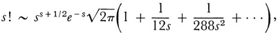
a result that can be obtained as well from Stirling’s approximation to log s! (Chap. 20, sec. 4).
Laplace had occasion, in his Théorie analytique des probabilités,5 to consider integrals of the form
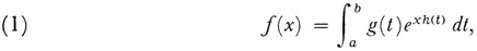
where g may be complex, h and t are real, and x is large and positive; he remarked that the main contribution to the integral comes from the immediate neighborhood of those points in the range of integration in which h(t) attains its absolute maximum. The contribution of which Laplace spoke is the first term of what we would call today an asymptotic series evaluation of the integral. If h(t) has just one maximum at t = a, then Laplace’s result is
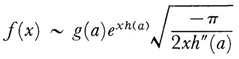
as x approaches ∞.
If in place of (1) the integral to be evaluated is
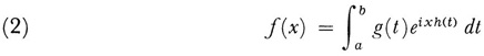
when t and x are real and x is large, then |eixh(t)| is a constant and Laplace’s method does not apply. In this case a method adumbrated by Cauchy in his major paper on the propagation of waves,6 now called the principle of stationary phase, is applicable. The principle states that the most relevant contribution to the integral comes from the immediate neighborhoods of the stationary points of h(t), that is, the points at which h’(t) = 0. This principle is intuitively reasonable because the integrand can be thought of as an oscillating current or wave wilh amplitude |g(t)|. If t is time, then the velocity of the wave is proportional to xh’(t), and if h’(t) ≠ 0, the velocity of the oscillations increases indefinitely as x becomes infinite. The oscillations are then so rapid that during a full period g(t) is approximately constant and xh(t) is approximately linear, so that the integral over a full period vanishes. This reasoning fails at a value of t where h’(t) = 0. Thus the stationary points of h(t) are likely to furnish the main contribution to the asymptotic value of f(x). If τ is a value of t at which h’(t) = 0 and h"(τ) > 0, then
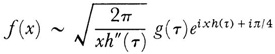
as x becomes infinite.
This principle was used by Stokes in evaluating Airy’s integral (see below) in a paper of 18567 and was formulated explicitly by Lord Kelvin.8 The first satisfactory proof of the principle was given by George N. Watson (1886-1965).9
In the first few decades of the nineteenth century, Cauchy and Poisson evaluated many integrals containing a parameter in series of powers of the parameter. In the case of Poisson the integrals arose in geophysical heat conduction and elastic vibration problems, whereas Cauchy was concerned with water waves, optics, and astronomy. Thus Cauchy, working on the diffraction of light,10 gave divergent series expressions for the Fresnel integrals:
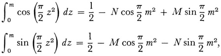
where

During the nineteenth century several other methods, such as the method of steepest descent, were invented to evaluate integrals. The full theory of all these methods and the proper understanding of what the approximations amounted to, whether single terms or full series, had to await the creation of the theory of asymptotic series.
Many of the integrals that were expanded by the above-described methods arose first as solutions of differential equations. Another use of divergent series was to solve differential equations directly. This use can be traced back at least as far as Euler’s work11 wherein, concerned with solving the non-uniform vibrating-string problem (Chap. 22, sec. 3), he gave an asymptotic series solution of an ordinary differential equation that is essentially Bessel’s equation of order r/2, where r is integral.
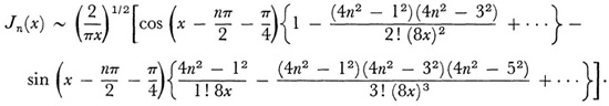
Jacobi12 gave the asymptotic form of Jn(x) for large x:
A somewhat different use of divergent series in the solution of differential equations was introduced by Liouville. He sought13 approximate solutions of the differential equation
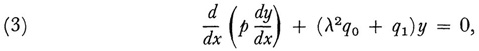
where p, q0, and q1 are positive functions of x and λ is a parameter; the solution is to be obtained in a ≤ x ≤ b. Here, as opposed to boundary-value problems where discrete values of λ are sought, he was interested in obtaining some approximate form of y for large values of λ. To do this he introduced the variables
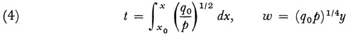
and obtained
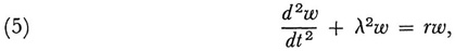
where
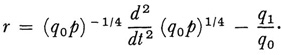
He then used a process that amounts in modern language to the solution by successive approximations of an integral equation of the Volterra type, namely,
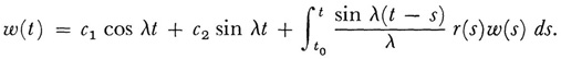
Liouville now argued that for sufficiently large values of λ the first approximation to the solutions of (5) should be

If the values of ω and l given by (4) are now used to obtain the approximate solution of (3), we have from (6) that

Though Liouville was not aware of it, he had obtained the first term of an asymptotic series solution of (3) for large λ
The same method was used by Green14 in the study of the propagation of waves in a channel. The method has been generalized slightly to equations of the form

in which λ is a large positive parameter and x may be real or complex. The solutions are now usually expressed as

The error term 0(l/λ) implies that the exact solution would contain a term F(x, λ)/λ where |F(x, λ)| is bounded for all x in the domain under consideration and for λ > λ0. The form of the error term is valid in a restricted domain of the complex x-plane. Liouville and Green did not supply the error term or conditions under which their solutions were valid. The more general and precise approximation (9) is explicit in papers by Gregor Wentzel (1898-),15 Hendrik A. Kramers (1894-1952),16 Léon Brillouin (1889-1969),17 and Harold Jeffreys (1891-1989),18 and is familiarly known as the WKBJ solution. These men were working with Schrodinger’s equation in quantum theory.
In a paper read in 1850,19 Stokes considered the value of Airy’s integral
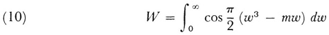
for large |m|. This integral represents the strength of diffracted light near a caustic. Airy had given a series for W in powers of m which, though convergent for all m, was not useful for calculation when |m| is large. Stokes’s method consisted in forming a differential equation of which the integral is a particular solution and solving the differential equation in terms of divergent series that might be useful for calculation (he called such series semiconvergent).
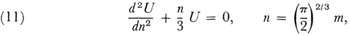
After showing that U = (π/2)1:3 W satisfies the Airy differential equation
Stokes proved that for positive n
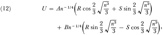


The quantities A and B that make U yield the integral were determined by a special argument (wherein Stokes uses the principle of stationary phase). He also gave an analogous result for n negative.
The series (12) and the one for negative n behave like convergent series for some number of terms but are actually divergent. Stokes observed that they can be used for calculation. Given a value of n, one uses the terms from the first up to the one that becomes smallest for the value of n in question. He gave a qualitative argument to show why the series are useful for numerical work.
Stokes encountered a special difficulty with the solutions of (11) for positive and negative n. He was not able to pass from the series for which n is positive to the series for which n is negative by letting n vary through 0 because the series have no meaning for n = 0. He therefore tried to pass from positive to negative n through complex values of n, but this did not yield the correct series and constant multipliers.
What Stokes did discover, after some struggle,20 was that if for a certain range of the amplitude of n a general solution was represented by a certain linear combination of two asymptotic series each of which is a solution, then in a neighboring range of the amplitude of n it was by no means necessary for the same linear combination of the two fundamental asymptotic expansions to represent the same general solution. He found that the constants of the linear combination changed abruptly as certain lines given by amp. n = const, were crossed. These are now called Stokes lines.
Though Stokes had been primarily concerned with the evaluation of integrals, it was clear to him that divergent series could be used generally to solve differential equations. Whereas Euler, Poisson, and others had solved individual equations in such terms, their results appeared to be tricks that produced answers for specific physical problems. Stokes actually gave several examples in the 1856 and 1857 papers.
The above work on the evaluation of integrals and the solution of differential equations by divergent series is a sample of what was done by many mathematicians and physicists.
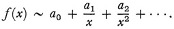
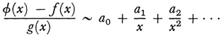
The full recognition of the nature of those divergent series that are useful in the representation and calculation of functions and a formal definition of these series were achieved by Poincaré and Stieltjes independently in 1886. Poincaré called these series asymptotic while Stieltjes continued to use the term semiconvergent. Poincaré21 took up the subject in order to further the solution of linear differential equations. Impressed by the usefulness of divergent series in astronomy, he sought to determine which were useful and why. He succeeded in isolating and formulating the essential property. A series of the form

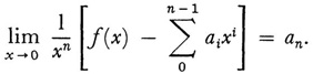
where the a1, are independent of x, is said to represent the function f(x) asymptotically for large values of x whenever

for n = 0, 1, 2, 3,. … The series is generally divergent but may in special cases be convergent. The relationship of the series to f(x) is denoted by
Such series are expansions of functions in the neighborhood of x = ∞. Poincaré in his 1886 paper considered real x-values. However, the definition holds also for complex x if x → ∞. is replaced by |x| → ∞, though the validity of the representation may then be confined to a sector of the complex plane with vertex at the origin.
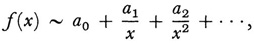
The series (15) is asymptotic to f(x) in the neighborhood of x = ∞. However, the definition has been generalized, and one speaks of the series
a0 + a1x + a2x2 + …
as asymptotic to f(x) at x = 0 if
Though in the case of some asymptotic series one knows what error is committed by stopping at a definite term, no such information about the numerical error is known for general asymptotic series. However, asymptotic series can be used to give rather accurate numerical results for large x by employing only those terms for which the magnitude of the terms decreases as one takes more and more terms. The order of the magnitude of the error at any stage is equal to the magnitude of the first term omitted.
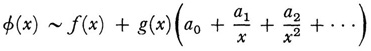
Poincaré proved that the sum, difference, product, and quotient of two functions are represented asymptotically by the sum, difference, product, and quotient of their separate asymptotic series, provided that the constant term in the divisor series is not zero. Also, if
then
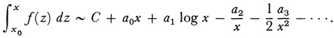
The use of integration involves a slight generalization of the original definition, namely,
if
even when f(x) and g(x) do not themselves have asymptotic series representations. As for differentiation, if f’(x) is known to have an asymptotic series expansion, then it can be obtained by differentiating the asymptotic series for f(x).
If a given function has an asymptotic series expansion it is unique, but the converse is not true because, for example, (1 + x)-1 and (1 + e-x). (l + x)-1 have the same asymptotic expansion.
Poincaré applied his theory of asymptotic series to differential equations, and there are many such uses in his treatise on celestial mechanics, Les Méthodes nouvelles de la mécanique céleste.22 The class of equations treated in his 1886 paper is

where the Pt(x) are polynomials in x. Actually Poincaré treated only the second order case but the method applies to (17).
The only singular points of equation (17) are the zeros of Pn(x) and x = ∞. For a regular singular point (Stelle der Bestimmtheit) there are convergent expressions for the integrals given by Fuchs (Chap. 29, sec. 5). Consider then an irregular singular point. By a linear transformation this point can be removed to ∞, while the equation keeps its form. If Pn is of the pth degree, the condition that x = ∞ shall be a regular singular point is that the degrees of Pn - 1, Pn -2, … P0 be at most P – 1, P – 2, …, P – n respectively. For an irregular singular point one or more of these degrees must be greater. Poincaré showed that for a differential equation of the form (17), wherein the degrees of the Pi do not exceed the degree of Pn, there exist n series of the form
and the series satisfy the differential equation formally. He also showed that to each such series there corresponds an exact solution in the form of an integral to which the series is asymptotic.
Poincaré’s results are included in the following theorem due to Jakob Horn (1867-1946).23 He treats the equation

where the coefficients are rational functions of x and are assumed to be developable for large positive x in convergent or asymptotic series of the form

k being some positive integer or 0. If for the above equation (18) the roots m1, m2, … mn of the characteristic equation, that is, the algebraic equation
mn + a1, 0mn - 1 + … + an, 0 = 0,
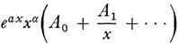
are distinct, equation (18) possesses n linearly independent solutions y1, y2, …, yn which are developable asymptotically for large positive values of x in the form

where fr(x) is a polynomial of degree k + 1 in x, the coefficient of whose highest power in x is mr/(k + 1), while ρr and Ar, j are constants with Ar, 0 = 1. The results of Poincaré and Horn have been extended to various other types of differential equations and generalized by inclusion of the cases where the roots of the characteristic equation are not necessarily distinct.
The existence, form, and range of the asymptotic series solution when the independent variable in (18) is allowed to take on complex values was first taken up by Horn.24 A general result was given by George David Birkhoff (1884-1944), one of the first great American mathematicians.25 Birkhoff in this paper did not consider equation (18) but the more general system
in which for |x| > R we have for each aij

and for which the characteristic equation in α
|aij – δijα| = 0
has distinct roots. He gave asymptotic series solutions for the y1 which hold in various sectors of the complex plane with vertices at x = 0.
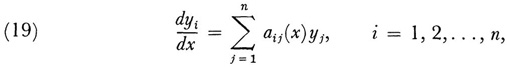
Whereas Poincaré’s and the other expansions above are in powers of the independent variable, further work on asymptotic series solutions of differential equations turned to the problem first considered by Liouville (sec. 2) wherein a parameter is involved. A general result on this problem was given by Birkhoff.26 He considered

for large |p| and for x in the interval [a, b]. The functions ai,(x, ρ) are supposed analytic in the complex parameter ρ at ρ = ∞ and have derivatives of all orders in the real variable x. The assumptions on ai(x, p) imply that
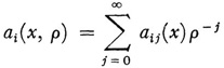
and that the roots of ω1(x), ω2(x), …, ωn(x) of the characteristic equation
ωn + an - 1,0(x)ωπ - 1 + … + a00(x) = 0
are distinct for each x. He proves that there are n independent solutions
z1(x, ρ), …, zn(x, ρ)
of (20) that are analytic in p in a region S of the p plane (determined by the argument of p), such that for any integer m and large |p|

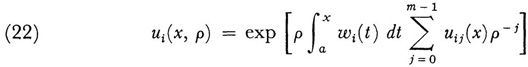
and E0 is a function of x, p, and m bounded for all x in [a, b] and p in S. The uij(x) are themselves determinable. The result (21), in view of (22), states that zi is given by a series in 1/p up to 1/ρm - 1 plus a remainder term, namely, the second term on the right, which contains 1/ρm. Moreover, since m is arbitrary, one can take as many terms in 1/ρ as one pleases into the expression for ui(x, p). Since E0 is bounded, the remainder term is of higher order in 1/ρ than ui(x, ρ). Then the infinite series, which one can obtain by letting m become infinite, is asymptotic 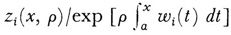 in Poincaré’s sense.
In Birkhoff’s theorem the asymptotic series for complex p is valid only in a sector S of the complex p plane. The Stokes phenomenon enters. That is, the analytic continuation of zi(x, ρ) across a Stokes line is not given by the analytic continuation of the asymptotic series for zi(x, p).
The use of asymptotic series or of the WKBJ approximation to solutions of differential equations has raised another problem. Suppose we consider the equation

where x ranges over [a, b]. The WKBJ approximation for large λ in view of (7), gives two solutions for x > 0 and two for x < 0. It breaks down at the value of x where q = 0. Such a point is called a transition point, turning point, or Stokes point. The exact solutions of (23) are, however, finite at such a point. The problem is to relate the WKBJ solutions on each side of the transition point so that they represent the same exact solution over the interval [a, b] in which the differential equation is being solved. To put the problem more specifically, consider the above equation in which q(x) is real for real x and such that q(x) = 0, q’(x) ≠ 0 for x = 0. Suppose also that q(x) is negative for x positive (or the reverse). Given a linear combination of the two WKBJ solutions for x < 0 and another for x > 0, the question arises as to which of the solutions holding for x > 0 should be joined to that for x < 0. Connection formulas provide the answer.
The scheme for crossing a zero of q(x) was first given by Lord Rayleigh27 and extended by Richard Gans (1880-1954),28 who was familiar with Rayleigh’s work. Both of these men were working on the propagation of light in a varying medium.
The first systematic treatment of connection formulas was given by Harold Jeffreys29 independently of Gans’s work. Jeffreys considered the equation
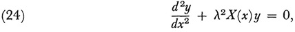
where x is real, λ is large and real, and X(x) has a simple zero at, say, x = 0. He derived formulas connecting the asymptotic series solutions of (24) for x > 0 and x < 0 by using an approximating equation for (24), namely,
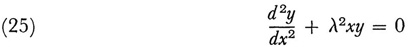
which replaces X(x) in (24) by a linear function in x. The solutions of (25) are

where ξ = (2/3)λx3/2, The asymptotic expansions for large x of these solutions can be used to join the asymptotic solutions of (24) on each side of x = 0. There are many details on the ranges of x and λ that must be considered in the joining process but we shall not enter into them. Extension of the work on connection formulas for the cases where X(x) in (24) has multiple zeros or several distinct zeros and for more complicated second order and higher-order equations and for complex x and λ has appeared in numerous papers.
The theory of asymptotic series, whether used for the evaluation of integrals or the approximate solution of differential equations, has been extended vastly in recent years. What is especially worth noting is that the mathematical development shows that the eighteenth- and nineteenth-century men, notably Euler, who perceived the great utility of divergent series and maintained that these series could be used as analytical equivalents of the functions they represented, that is, that operations on the series corresponded to operations on the functions, were on the right track. Even though these men failed to isolate the essential rigorous notion, they saw intuitively and on the basis of results that divergent series were intimately related to the functions they represented.
The work on divergent series described thus far has dealt with finding asymptotic series to represent functions either known explicitly or existing implicitly as solutions of ordinary differential equations. Another problem that mathematicians tackled from about 1880 on is essentially the converse of finding asymptotic series. Given a series divergent in Cauchy’s sense, can a “sum” be assigned to the series? If the series consists of variable terms this “sum” would be a function for which the divergent series might or might not be an asymptotic expansion. Nevertheless the function might be taken to be the “sum” of the series, and this “sum” might serve some useful purposes, even though the series will certainly not converge to it or may not be usable to calculate approximate values of the function.
To some extent the problem of summing divergent series was actually undertaken before Cauchy introduced his definitions of convergence and divergence. The mathematicians encountered divergent series and sought sums for them much as they did for convergent series, because the distinction between the two types was not sharply drawn and the only question was, What is the appropriate sum? Thus Euler’s principle (Chap. 20, sec. 7) that a power series expansion of a function has as its sum the value of the function from which the series is derived gave a sum to the series even for values of x for which the series diverges in Cauchy’s sense. Likewise, in his transformation of series (Chap. 20, sec. 4), he converted divergent series to convergent ones without doubting that there should be a sum for practically all series. However, after Cauchy did make the distinction between convergence and divergence, the problem of summing divergent series was broached on a different level. The relatively naive assignments in the eighteenth century of sums to all series were no longer acceptable. The new definitions prescribe what is now called summability, to distinguish the notion from convergence in Cauchy’s sense.
With hindsight one can see that the notion of summability was really what the eighteenth- and early nineteenth-century men were advancing. This is what Euler’s methods of summing just described amount to. In fact in his letter to Goldbach of August 7, 1 745, in which he asserted that the sum of a power series is the value of the function from which the series is derived, Euler also asserted that every series must have a sum, but since the word sum implies the usual process of adding, and this process does not lead to the sum in the case of a divergent series such as 1 — 1! + 2! — 3! + …, we should use the word value for the “sum” of a divergent series.
Poisson too introduced what is now recognized to be a summability notion. Implied in Euler’s definition of sum as the value of the function from which the series comes is the idea that
(The notation 1 — means that x approaches 1 from below.) According to (27) the sum of 1 - 1 + 1 - 1 + … is

Poisson30 was concerned with the series
sin θ + sin 2θ + sin 3θ + …
which diverges except when θ is a multiple of π. His concept, expressed for the full Fourier series
is that one should consider the associated power series
and define the sum of (28) to be the limit of the series (29) as r approaches 1 from below. Of course Poisson did not appreciate that he was suggesting a definition of a sum of a divergent series because, as already noted, the distinction between convergence and divergence was in his time not a critical one.
The definition used by Poisson is now called Abel summability because it was also suggested by a theorem due to Abel,31 which states that if the power series
has a radius of convergence r and converges for x = r, then
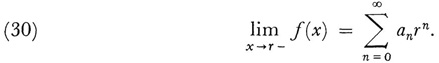
Then the function f(x) defined by the series in –r < x ≤ r is continuous on the left at x = r. However, if Σ an does not converge and the limit (30) does exist for r = 1, then one has a definition of sum for the divergent series. This formal definition of summability for series divergent in Cauchy’s sense was not introduced until the end of the nineteenth century in a connection soon to be described.
One of the motivations for reconsidering the summation of divergent series, beyond their continued usefulness in astronomical work, was what has been called the boundary-value (Grenzwert) problem in the theory of analytic functions. A power series Σ anxn may represent an analytic function in a circle of radius r but not for values of x on the circle. The problem was whether one could find a concept of sum such that the power series might have a sum for |x| = r and such that this sum might even be the value of f(x) as |x| approaches r. It was this attempt to extend the range of the power series representation of an analytic function that motivated Frobenius, Hölder, and Ernesto Cesàro. Frobenius32 showed that if the power series Σ anxn has the interval of convergence -1 < x < 1, and if
(31) sn = a0 + a1 + … + an,
then
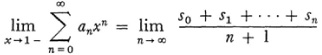
when the right-hand limit exists. Thus the power series normally divergent for x = 1 can have a sum. Moreover if f(x) is the function represented by the power series, Frobenius’s definition of the value of the series at x = 1 agrees with limx → 1 - f(x).
Divorced from its connection with power series, Frobenius’s work suggested a summability definition for divergent series. If Σ an is divergent and sn has the meaning in (31), then one can take as the sum
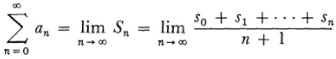
if this limit exists. Thus for the series 1 – 1 + 1 – ! + …, the Sn have the values 1, 1/2, 2/3, 2/4, 3/5, 1/2, 4/7, 1/2,… so that limn → ∞ Sn = 1/2. If Σ an converges, then Frobenius’s “sum” gives the usual sum. This idea of averaging the partial sums of a series can be found in the older literature. It was used for special types of series by Daniel Bernoulli33 and Joseph L. Raabe (1801-59).34
Shortly after Frobenius published his paper, Hölder35 produced a generalization. Given the series Σ an let
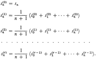

if this limit exists for some τ. Hölder’s definition is now known as summability (H, r).
Hölder gave an example. Consider the series
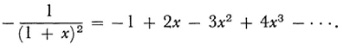
This series diverges when x = 1. However for x = 1,
s0 = -1, s1 = 1, s2 = -2, s3 = 2, s4 = -3, ….
Then
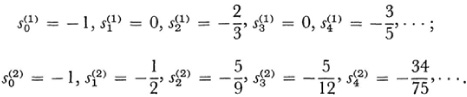
It is almost apparent that 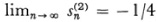 , and this is the Hölder sum (H, 2). It is also the value that Euler assigned to the series on the basis of his principle that the sum is the value of the function from which the series is derived.
Another of the now-standard definitions of summability was given by Cesàro, a professor at the University of Naples.36 Let the series be  and let sn be
  . Then the Cesàro sum is
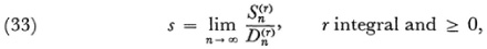
where

and
The case r = 1 includes Frobenius’s definition. Cesàro’s definition is now referred to as summability (C, r). The methods of Hölder and Cesàro give the same results. That Hölder summability implies Cesàro’s was proved by Konrad Knopp (1882-1957) in an unpublished dissertation of 1907; the converse was proved by Walter Schnee (b. 1885).37
An interesting feature of some of the definitions of summability when applied to power series with radius of convergence 1 is that they not only give a sum that agrees with limx → 1 - f(x), where f(x) is the function whose power series representation is involved, but have the further property that they preserve a meaning in regions where |x| > 1 and in these regions furnish the analytic continuation of the original power series.
Further progress in finding a “sum” for divergent series received its motivation from a totally different direction, the work of Stieltjes on continued fractions. The fact that continued fractions can be converted into divergent or convergent series and conversely was utilized by Euler.38 Euler sought (Chap. 20, sees. 4 and 6) a sum for the divergent series

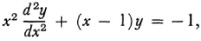
In his article on divergent series39 and in correspondence with Nicholas Bernoulli (1687-1759),40 Euler first proved that

formally satisfies the differential equation
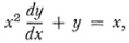
for which he obtained the integral solution
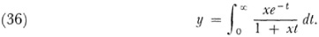
Then by using rules he derived for converting convergent series into continued fractions Euler transformed (35) into
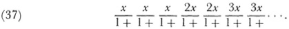
This work contains two features. On the one hand, Euler obtained an integral that can be taken to be the “sum” of the divergent series (35); the latter is in fact asymptotic to the integral. On the other hand he showed how to convert divergent series into continued fractions. In fact he used the continued fraction for x = 1 to calculate a value for the series (34).
There was incidental work of this nature during the latter part of the eighteenth century and a good deal of the nineteenth, of which the most noteworthy is due to Laguerre.41 He proved, first of all, that the integral (36) could be expanded into the continued fraction (37). He also treated the divergent series

Since
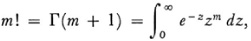
the series can be written as
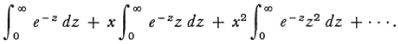
If we formally interchange summation and integration we obtain
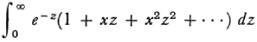
or
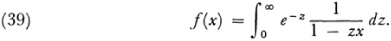
The f(x) thus derived is analytic for all complex x except real and positive values and can be taken to be the “sum” of the series (38).
In his thesis of 1886 Stieltjes took up the study of divergent series.42 Here Stieltjes introduced the very same definition of a series asymptotic to a function that Poincaré had introduced, but otherwise confined himself to the computational aspects of some special series.
Stieltjes did go on to study continued fraction expansions of divergent series and wrote two celebrated papers of 1894-95 on this subject.43 This work, which is the beginning of an analytic theory of continued fractions, considered questions of convergence and the connect’on with definite integrals and divergent series. It was in these papers that he introduced the integral bearing his name.
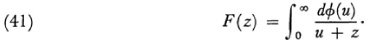
Stieltjes starts with the continued fraction

where the an arc positive real numbers and z is complex. He then shows that when the series Σ∞n = 1 an diverges, the continued fraction (40) converges to a function F(z) which is analytic in the complex plane except along the negative real axis and at the origin, and
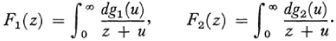
When Σ an converges, the even and odd partial sums of (40) converge to distinct limits F1(z) and F2(z) where
Now it was known that the continued fraction (40) could be formally developed into a series
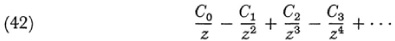
with positive Ci. The correspondence (with some restrictions) is also reciprocal. To every series (42) there corresponds a continued fraction (40) with positive an. Stieltjes showed how to determine the Ci from the an and in the case where Σ an is divergent he showed that the ratio Cn/Cn -1 increases. If it has a finite limit λ, the series converges for |z| > λ, but if the ratio increases without limit then the series diverges for all z.
The relation between the series (42) and the continued fraction (40) is more detailed. Although the continued fraction converges if the series does, the converse is not true. When the series (42) diverges one must distinguish two cases, according as Σ an is divergent or convergent. In the former case, as we have noted, the continued fraction gives one and only one functional equivalent, which can be taken to be the sum of the divergent series (42). When Σ an is convergent two different functions are obtained from the continued fraction, one from the even convergents and the other from the odd convergents. But to the series (42) (now divergent) there corresponds an infinite number of functions each of which has the series as its asymptotic development.
Stieltjes’s results have also this significance: they indicate a division of divergent series into at least two classes, those series for which there is properly a single functional equivalent whose expansion is the series and those for which there are at least two functional equivalents whose expansions are the series. The continued fraction is only the intermediary between the series and the integral; that is, given the series ore obtains the integral through the continued fraction. Thus, a divergent series belongs to one or more functions, which functions can be taken to be the sum of the series in a new sense of sum.
Stieltjes also posed and solved an inverse problem. To simplify the statement a bit, let us suppose that φ(u) is differentiable so that the integral(41) can be written as
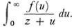
To the divergent series (42) and in the case where Σ an is divergent there corresponds an integral of this form. The problem is, given the series to find f(u). A formal expansion of the integral shows that

Hence knowing the Cn one must determine f(u) satisfying the infinite set of equations (43). This is what Stieltjes called the “problem of moments.” It does not admit a unique solution, for Stieltjes himself gave a function
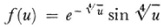
which makes Cn = 0 for all n. If the supplementary condition is imposed that f(u) shall be positive between the limits of integration, then only a single f(u) is possible.
The systematic development of the theory of summable series begins with the work of Borel from 1895 on. He first gave definitions that generalize Cesàro’s. Then, taking off from Stieltjes’s work, he gave an integral definition.44 If the process used by Laguerre is applied to any series of the form

having a finite radius of convergence (including 0), we are led to the integral
where
This integral is the expression on which Borel built his theory of divergent series. It was taken by Borel to be the sum of the series (44). The series F(u) is called the associated scries of the original series.
If the original series (44) has a radius of convergence R greater than 0, the associated series represents an entire function. Then the integral  has a sense if x lies within the circle of convergence, and the values of the integral and series are identical. But the integral may have a sense for values of x outside the circle of convergence, and in this case the integral furnishes an analytic continuation of the original series. The series is said by Borel to be summable (in the sense just explained) at a point x where the integral has a meaning.
If the original series (44) is divergent (R = 0), the associated series may be convergent or divergent. If it is convergent over only a portion of the plane u = zx we understand by F(u) the value not merely of the associated series but of its analytic continuation. Then the integral  may have a meaning and is, as we sec, obtained from the original divergent series. The determination of the region of ^-values in which the original series is summable was undertaken by Borel, both when the original series is convergent (R > 0) and divergent (R = 0).
Borel also introduced the notion of absolute summability. The original series is absolutely summable at a value of x when
is absolutely convergent and the successive integrals
have a sense. Borel then shows that a divergent series, if absolutely summable, can be manipulated precisely as a convergent series. The series, in other words, represents a function and can be manipulated in place of the function. Thus the sum, difference, and product of two absolutely summable series is absolutely summable and represents the sum, difference, and product respectively of the two functions represented by the separate series. The analogous fact holds for the derivative of an absolutely summable series. Moreover the sum in the above sense agrees with the usual sum in the case of a convergent series, and subtraction of the first k terms reduces the “sum” of the entire series by the sum of these k terms. Borel emphasized that any satisfactory definition of summability must possess these properties, though not all do. He did not require that any two definitions necessarily yield the same sum.
These properties made possible the immediate application of Borel’s theory to differential equations. If, in fact,
P(x, y, y', … y(n)) = 0
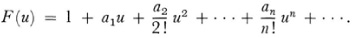
is a differential equation which is holomorphic in x at the origin and is algebraic in y and its derivatives, any absolutely summable series
a0 + a1x + a2x2 + …
which satisfies the differential equation formally defines an analytic function that is a solution of the equation. For example, the Laguerre series
1 + x + 2!x2 + 3!x3 + …
and so the function (ef. (39))
must be a solution of the equation.
Once the notion of summability gained some acceptance, dozens of mathematicians introduced a variety of new definitions that met some or all of the requirements imposed by Borel and others. Many of the definitions of summability have been extended to double series. Also, a variety of problems has been formulated and many solved that involve the notion of summability. For example, suppose a series is summable by some method. What additional conditions can be imposed on the series so that, granted its summability, it will also be convergent in Cauchy’s sense? Such theorems are called Tauberian after Alfred Tauber (1866—1942?). Thus Tauber proved45 that if Σ an, is Abelian summable to s and nan approaches 0 as n becomes infinite, then Σ an converges to s.
The concept of summability does then allow us to give a value or sum to a great variety of divergent series. The question of what is accomplished thereby necessarily arises. If a given infinite series were to arise directly in a physical situation, the appropriateness of any definition of sum would depend entirely on whether the sum is physically significant, just as the physical utility of any geometry depends on whether the geometry describes physical space. Cauchy’s definition of sum is the one that usually fits because it says basically that the sum is what one gets by continually adding more and more terms in the ordinary sense. But there is no logical reason to prefer this concept of sum to the others that have been introduced. Indeed the representation of functions by series is greatly extended by employing the newer concepts. Thus Leopold Fejer (1880-1959), a student of H. A. Schwarz, showed the value of summability in the theory of Fourier series. In 190446 Fejér proved that if in the interval [– π, π], f(x) is bounded and (Riemann) integrable, or if unbounded the integral  is absolutely convergent, then at every point in the interval at which f(x + 0) and f(x – 0) exist, the Frobenius sum of the Fourier series
is [f(x + 0) + f(x – 0)]/2. The conditions on f(x] in this theorem are weaker than in previous theorems on the convergence of Fourier series to f(x) (cf. Chap. 40, sec. 6).
Fejér’s fundamental result was the beginning of an extensive series of fruitful investigations on the summability of series. We have had numerous occasions to view the need to represent functions by infinite series. Thus in meeting the initial condition in the solution of initial- and boundary-value problems of partial differential equations, it is usually necessary to represent the given initial f(x) in terms of the eigenfunctions that are obtained from the application of the boundary conditions to the ordinary differential equations that result from the method of separation of variables. These eigenfunctions can be Bessel functions, Legendre functions, or any one of a number of types of special functions. Whereas the convergence in the Cauchy sense of such a series of eigenfunctions to the given f(x) may not obtain, the series may indeed be summable tof(x) in one or another of the senses of summability and the initial condition is thereby satisfied. These applications of summability represent a great success for the concept.
The construction and acceptance of the theory of divergent series is another striking example of the way in which mathematics has grown. It shows, first of all, that when a concept or technique proves to be useful even though the logic of it is confused or even nonexistent, persistent research will uncover a logical justification, which is truly an afterthought. It also demonstrates how far mathematicians have come to recognize that mathematics is man-made. The definitions of summability are not the natural notion of continually adding more and more terms, the notion which Cauchy merely rigorized; they are artificial. But they serve mathematical purposes, including even the mathematical solution of physical problems; and these are now sufficient grounds for admitting them into the domain of legitimate mathematics.
Borel, Emile: Notice sur les travaux scientifiques de M. Emile Borel, 2nd ed., GauthierVillars, 1921.
———: Leçons sur les séries divergentes, Gauthier-Villars, 1901.
Burkhardt, H.: “Trigonometrische Reihe und Integrate,” Encyk. der Math. Wiss., B. G. Teubner, 1904-16, II A12, 819-1354.
———: “Über den Gebrauch divergenter Reihen in der Zeit von 1750-1860,” Math. Ann., 70, 1911, 169-206.
Carmichael, Robert D.: “General Aspects of the Theory of Summable Series,” Amer. Math. Soc. Bull., 25, 1918/19, 97-131.
Collingwood E. F.: “Emile Borel,” Jour. Lon. Math. Soc., 34, 1959, 488-512.
Ford, W. B.: “A Conspectus of the Modern Theories of Divergent Series,” Amer. Math. Soc. Bull., 25, 1918/19, 1-15.
Hardy, G. H.: Divergent Series, Oxford University Press, 1949. See the historical notes at the ends of the chapters.
Hurwitz, W. A.: “A Report on Topics in the Theory of Divergent Series,” Amer. Math. Soc. Bull., 28, 1922, 17-36.
Knopp, K.: “Neuere Untersuchungen in der Theorie der divergenten Reihen,” Jahres. der Deut. Math.-Verein., 32, 1923, 43-67.
Langer, Rudolf E.: “The Asymptotic Solution of Ordinary Linear Differential Equations of the Second Order,” Amer. Math. Soc. Bull., 40, 1934, 545-82.
McHugh, J. A. M.: “An Historical Survey of Ordinary Linear Differential Equations with a Large Parameter and Turning Points,” Archive for History of Exact Sciences, 7, 1971, 277-324.
Moore, C. N.: “Applications of the Theory of Summability to Developments in Orthogonal Functions,” Amer. Math. Soc. Bull., 25, 1918/19, 258-76.
Plancherel, Michel: “Le Développement de la théorie des séries trigonométriques dans le dernier quart de siècle,” L’Enseignement Mathématique, 24, 1924/25, 19-58.
Pringsheim, A.: “Irrationalzahlen und Konvergenz unendlicher Prozesse,” Encyk. der Math. Wiss., B. G. Teubner, 1898-1904, IA3, 47-146.
Reiff, R.: Geschichte der unendlichen Reihen, H. Lauppsche Buchhandlung, 1889, Martin Sandig (reprint), 1969.
Smail, L. L.: History and Synopsis of the Theory of Summable Infinite Processes, University of Oregon Press, 1925.
Van Vleck, E. B.: “Selected Topics in the Theory of Divergent Series and Continued Fractions,” The Boston Colloquium of the Amer. Math. Soc., 1903, Macmillan, 1905, 75-187.