6 BULLS AND BEARS
PREDICTING OUR ECONOMY

Rules by their nature are simple. Our problem is not the complexity of our models but the far greater complexity of a world economy whose underlying linkages appear to be in a continual state of flux.

—Alan Greenspan, chairman of the U.S. Federal Reserve (1987–2006)

To me our knowledge of the way things work, in society or in nature, comes trailing clouds of vagueness.

—Kenneth Arrow, Nobel laureate in economics

ANATOMY OF A STORM

In 1720, an entrepreneur set up a company in England for the mysterious purpose of “carrying on an undertaking of great advantage, but nobody to know what it is.” Five thousand shares of £100 would be issued. The public could get in at the ground floor by making a deposit of £2 per share. In a month’s time, the technical details of the project would be filled in and a call made for the remaining £98. The promised payoff was generous: £100 per year, per share.

The next morning, the man opened his office in London’s financial district to admit the deluge of investors who were waiting outside. At the end of the day, he counted his takings, saw he had sold a thousand shares, and promptly left for Europe.1

In the same year, other company prospectuses offered even less investor value. One tried to raise a million pounds to fund the development of a “wheel of perpetual motion”; others promoted techniques for “extracting silver from lead,” and for turning “quicksilver into a malleable fine metal.” But the one that caused the most damage, and created the almost hysterical environment for these “bubble” investments, as they came to be known, was a much larger project that was sanctioned by the highest levels of government, all the way up to King George I.

The South Sea Company was established in 1711 by Robert Harley, Earl of Oxford, to help fund the national debt. In return, it was granted a permanent monopoly on trade with Mexico and South America. Everyone knew these places harboured inexhaustible supplies of gold, and investors were easily found. The actual trading was slow to get started—the king of Spain restricted traffic to only one ship per year, and the first didn’t set sail until 1717—but the less that was delivered, the more enormous seemed the potential.

None of the company directors had experience with South Seas trade. Safely ensconced in their London office, they managed to arrange some slave-trade voyages, but these weren’t particularly profitable. Preferring to concentrate on financial schemes, and fuelled by the public’s love of gold, they made a bid to triple their share of the national debt to almost the full amount, at better terms than those offered by the Bank of England. Robert Walpole from the bank protested against the scheme, telling the House of Commons that it would “decoy the unwary to their ruin, by making them part with the earnings of their labour for a prospect of imaginary wealth.”

His Cassandra-like warnings went unheeded. Eased along by a number of large bribes, in the form of offerings of stock to politicians and influential people like King George’s mistresses, the company’s proposal was accepted by the government. Rumours of increasing Latin American trade spread like wildfire through the coffeehouses in Cornhill and Lombard streets, and in 1720 the stock rose yeastily, from £175 in February to over £1,000 by June. By then, scores of other businesses had been set up to cash in on the growing public interest in stock-market investment, which seemed to be making so many rich. As Charles Mackay, in his book Extraordinary Popular Delusions and the Madness of Crowds, commented: “The public mind was in a state of unwholesome fermentation. Men were no longer satisfied with the slow but sure profits of cautious industry.”

When the stock price crossed the four-figure barrier, the company directors, either spooked or sated, began to sell their shares. The price stabilized, then wobbled, then started to sink, as investors began to suspect they had been the victims of a giant scam. By the end of September, the price had collapsed to £135. As Jonathan Swift wrote:

Subscribers here by thousands float
And jostle one another down
Each paddling in his leaky boat
And here they fish for gold, and drown.2

Parliament was recalled to discuss the crisis. The bishop of Rochester called the scheme a “pestilence,” while Lord Molesworth suggested that the perpetrators be tied in sacks and thrown into the Thames. Robert Walpole was more contained, arguing that there would be time later to punish those responsible. “If the city of London were on fire, all wise men would aid in extinguishing the flames, and preventing the spread of the conflagration before they inquired after the incendiaries,” he remarked.

As they argued, the company treasurer Robert Knight put on a disguise, boarded a specially chartered boat, and slipped across the Channel to France. The former chancellor of the exchequer, John Aislabie, who was the company’s main advocate in the government, stayed to face the music and was escorted, Martha Stewart–fashion, to the Tower of London.

As a response to the crisis, which had caused a record number of bankruptcies at every level of society, Parliament passed the Bubble Act in 1721. It forbade the founding of joint-stock companies without a royal charter—but it didn’t manage to ban bubbles, or the occasional “irrational exuberance” of investors (as Alan Greenspan later described it). When the NASDAQ soared to new heights at the turn of the millennium, how many of its listed companies were engaged in an “undertaking of great advantage, but nobody to know what it is”? And could a trained scientist have predicted such rises and falls? Isaac Newton, who lost a large part of his fortune in the South Sea bubble, didn’t think so. As he said in 1721, “I can calculate the motions of heavenly bodies, but not the madness of people.”

Nonetheless, the gleaming skyscrapers of financial centres like London, New York, and Tokyo are full of professional prognosticators who make good money forecasting the future state of the economy. Is it therefore possible to build a dynamical model of the economy—a kind of global capital model—which is capable of forecasting economic storms? Given enough data and a large enough computer, can we predict the circulation of money just as we predict the orbit of Mars?

MAKING DOUGH

As Vilhem Bjerknes pointed out, the accuracy of a dynamical model depends on two things: the initial condition and the model itself. To know where the economy is going, we must first know its current state. In 1662, a London draper named John Graunt tried to do for his city what Tycho Brahe and other astronomers had done for the heavens: determine its population. His work Natural and Political Observations Made upon the Bills of Mortality compiled lists of births and deaths in London between 1604 and 1661. Many of the deaths were attributed either to lung disease, which Graunt associated with pollution from the burning of coal, or to outbreaks of the plague, like the one that forced the young Newton to leave Cambridge for the countryside.3

Graunt’s book can be seen as the beginning of the fields of sampling and demographics. The aim of sampling is to obtain estimates using a limited amount of information. Graunt used birth records to infer the number of women of child-bearing age. He then extrapolated to the total population, obtaining an estimate of 384,000 souls.

All measurements of the physical world contain a degree of uncertainty and error. To determine the average rainfall in a particular region, for example, we cannot count all the water that falls; instead, we’ll make use of a few randomly located rain-collection devices, each of which will give us a different reading. The average of these should be a good indicator of the region as a whole, provided the rainfall is reasonably uniform. When Tycho Brahe tried to measure the location of a distant star, this too was subject to error because of atmospheric distortions and because his measurements were done by eye. His sextant would give one answer one day, a slightly different answer the next. The “true” answer in such a situation is never known, so Tycho and other astronomers would take the average over different measurements. The sampling was done not over different stars, but over different measurement events.

Similarly, when pollsters want to estimate the average yearly income for a certain area, they ask a relatively small sample of people. So long as those selected are representative of the population as a whole, their responses can be used to make a statistical prediction of the likely average.

Given that all measurements are subject to uncertainty and error, how can we ever be sure that the answer we obtain is good enough? This question was addressed by mathematicians such as Jakob Bernoulli. Part of the famously talented Bernoulli clan, which was later studied by Galton as an example of inherited eminence, he imagined a jar containing a large number of white and black pebbles in a certain proportion to one another. We pull out one pebble, and it is black. The next is white. Then a black, and another black. Then three whites in a row. How many pebbles do we need to examine to make a good estimate of the true proportions? The answer was provided by Bernoulli’s law of large numbers, which showed that as more pebbles are sampled, their ratio will converge to the correct solution. In other words, sampling works for pebbles, so long as the sample is large enough.

Bernoulli believed that this result could be generalized beyond pebbles. He wrote, “If, instead of the jar, for instance, we take the atmosphere or the human body, which conceal within themselves a multitude of the most varied processes or diseases, just as the jar conceals the pebbles, then for these also we shall be able to determine by observation how much more frequently one event will occur than another.”⁴ Until then, the laws of probability had been limited to games of chance, where the odds of holding a face card or rolling two sixes, could be computed exactly. Using the techniques of sampling, it seemed, scientists could make probabilistic estimates of anything they wanted.

Sampling methods were put on a still firmer basis by de Moivre’s discovery of the bell curve, or normal distribution. His 1718 work, The Doctrine of Chances, which was dedicated to his London friend Isaac Newton, showed how, under certain conditions, a sample of random measurements will fall into the bell-shaped distribution, which peaks at the average value. As mentioned in the previous chapter, one of the most enthusiastic supporters of the normal distribution was Francis Galton, who described it as “the supreme law of Unreason” because events that appear random turn out to be governed by a simple mathematical rule.⁵ The mean (or average) and standard deviation of the curve can be used to determine the margin of error of a measurement or the expected range of a quantity based on a sample. Because mortality statistics tend to cluster according to a normal distribution, it was soon also used by insurance companies to determine life expectancies, and therefore to price annuities.

Galton’s work on inheritance drew on the research of the Belgian scientist Lambert Quetelet, who in his 1835 Treatise on Man and the Development of his Faculties, turned normal into a kind of character: l’homme moyen, or the average man. He claimed that “the greater the number of people observed, the more do peculiarities, whether physical or moral, become effaced, and allow the general facts to predominate, by which society exists and is preserved.”⁶ Perhaps this inspired Galton to make his composite photographs of convicts’ faces. It also seemed to put the social sciences on a footing similar to that of the physical sciences, which had made great strides by realizing that it is not necessary to model each particle in detail. The temperature of a gas is a function of the average motion of its individual molecules, so in a way it’s a measure of the “average molecule.” Perhaps a crowd of people could be similarly described by one average person, which would certainly make analysis easier.

Of course, while molecules of air are identical and don’t interact except by colliding, the same is not true of people. As the economist André Orléan observed, our “beliefs, interpretations and justifications evolve and transform themselves continuously.”⁷ If someone knocks on your door, says she is doing a survey, and asks how much money you earn in a year, you may tell her to go away, participate but lie because you are concerned that she is a tax officer in disguise, or say what you think is the truth but be wrong. If she asks how you feel about the economy, the answer may reveal your own strongly held opinions, but equally it may reflect a discussion you had the previous night or something you saw on a recent TV show. It will also depend on the exact way the question is asked. Just as in physics there is an uncertainty principle that states that the presence of the observer affects the outcome of an experiment, there is a corresponding demographic principle that says any answer is subjective and is affected by the questioner, and even by the language used. This is why politicians spend so much time arguing over how questions should be worded in referendums. Even exit polls are prone to error, as we saw in the 2004 U.S. election, when exit polls at first had John Kerry winning over George Bush.

In measuring the economy, about the only thing that can be counted on is money. An individual can count how much he earns; a company’s accountants can count how much it has produced; and a government’s accountants can count how much it has taxed. (Most societies undervalue things like trees because it is easy to calculate how much they’re worth when cut into pieces but much harder when they’re left intact. And trees don’t have accountants. This bias may change, to a degree, as economists try to invent costs for such “services.”⁸) Even counting money, however, is not straightforward. Governments constantly revise important data, such as unemployment figures and gross national product, and creative accounting techniques, like those used to value Internet companies in the 1990s, distort company accounts.

WHAT’S IT WORTH?

Demographics and accounting can give some insight into the current state of the economy, but to know where it is headed, we need to understand the dynamics of society, and in particular of money. Are there simple laws that underpin economics, like an analogue of Newton’s laws of motion for the movement of capital?

Such laws would obviously depend on the idea of value. Just as air flows from areas of high pressure to areas of low pressure, money flows through the economy, seeking out investments that are undervalued. The English philosopher Jeremy Bentham associated value with an object’s utility—the property that brings benefit to the owner.9 His follower, the economist William Stanley Jevons, noted that the utility of an agricultural commodity such as wheat depends on the amount available, which in turn is closely linked to the weather. If a harvest is ruined by drought, then bakers and others compete for the scarce resource, driving up the price. Jevons, who also produced meteorological works (including the first scientific study of the climate of Australia), believed that the weather was affected by sunspots. He therefore developed a model of the boom/bust business cycle based on the sunspot cycle. His hope was that economics would become “a science as exact as many of the physical sciences; as exact, for instance, as meteorology is likely to be for a very long time to come.”¹⁰

The desire to maximize utility is a kind of force that drives the economy. Again, though, there’s an important difference between utility and a physical property such as mass: the former is a dynamic quantity that for each person depends on her subjective expectations for the future. Financial transactions are based not just on present value but also on future value. In a market economy, where prices are not set by the state, future value is subject to a number of factors.

First, the value of an asset depends on its prospects for future growth. You don’t spend the asking price on a house if you suspect that in five years’ time its value will be diminished. Similarly, assets such as stocks can be redeemed only if the seller finds a buyer, which can be tricky if the company’s market evaporates overnight.

An asset’s valuation must also take into account its risk, which is related to its tendency to fluctuate. Suppose that instead of yeasts,figure 5.6 (see page 210) showed the historical returns from two assets, known as Regular and Mutant, over forty years. Since most people like to avoid unnecessary risk, if only so they can sleep at night, an asset that fluctuates greatly in price, like Mutant, is worth less than one that’s relatively stable. The volatility, usually denoted by σ, can be calculated from the standard deviation of the price fluctuations—assuming, of course, that these follow a normal distribution and the volatility does not change with time.

Finally, the value of money will also change, because of inflation and interest rates. If a stock pays a dividend of one dollar in a year’s time, and if inflation is zero and interest rates are 3 percent, then the “present value” of that dividend is ninety-seven cents (that’s how much you’d have to invest to receive a dollar in a year’s time). In economics, time really is money.

Calculating the present value of an asset is clearly a challenge. In the case of a stock, you have to estimate the company’s rate of growth, its volatility, any dividends, and the interest-rate environment— not just for now but into the future. Since none of these can be known by an investor who is less than clairvoyant, it means that the present value is at best a well-educated guess. Bonds at least pay you back, but only at some future date, by which time the value of money has changed. Even fixed interest-cash deposits are subject to the effects of inflation.

Assets that have limited functional use and do not earn interest, such as gold or diamonds, are considered valuable in part because of their beauty but mostly because of their scarcity. Galileo wrote, in Dialogue Concerning the Two Chief World Systems, “What greater stupidity can be imagined than that of calling jewels, silver, and gold ‘precious,’ and earth and soil ‘base’? People who do this ought to remember that if there were as great a scarcity of soil as of jewels or precious metals, there would not be a prince who would not spend a bushel of diamonds and rubies and a cartload of gold just to have enough earth to plant a jasmine in a little pot, or to sow an orange seed and watch it sprout, grow, and produce its handsome leaves, its fragrant flowers, and fine fruit.”¹¹ Adam Smith echoed him a century and a half later. “Nothing is more useful than water: but it will purchase scarce any thing; scarce any thing can be had in exchange for it,” he wrote. “A diamond, on the contrary, has scarce any value in use; but a very great quantity of other goods may frequently be had in exchange for it.”¹² Since the perceived scarcity depends on demand, it too is subject to the whims of the market.Value is therefore not a solid, intrinsic property, but is a fluid quality that changes with circumstances. The value of a bar of gold is determined not by its weight but by what the gold market will bear. Value in the end is decided by people, in a social process that depends on complex relationships in the marketplace. It is subjective rather than objective, moving rather than fixed. Indeed, we often seem more sensitive to changes in price than to the price itself (just watch what happens whenever the cost of gas spikes).

Because of this variability, it would seem that the economy could never reach equilibrium. Nonetheless, economists in the late nineteenth century reasoned that if the market were somehow to settle on a fixed price for each asset, which everyone agreed reflected its underlying “true” worth, then the future expectations of investors would align perfectly with the present. Furthermore, any small perturbation would be damped out by the negative feedback of Adam Smith’s invisible hand: the self-interest of “the butcher, the brewer, or the baker.” If the price of wheat was too high, then more producers would enter the market, driving the price back down. Fluctuations in prices would die out. Just as a molecule of gas has a known mass, every asset or object would have a fixed intrinsic value.

Of course, there will always be a constant flow of external shocks, new pieces of information that impact prices. In 2004, for example, North American bakeries had to deal with record cocoa prices caused by violence in the Ivory Coast; a rise in the cost per kilo for vanilla, owing in part to cyclones in Madagascar; high sugar prices caused by damage to crops in the Caribbean and the U.S.; expensive eggs because of avian flu; record oil prices, which affect transportation costs; and so on.¹³ All of these factors would affect a bakery’s bottom line, so the market would adjust its predictions about its performance. (Businesses often insulate themselves against such fluctuations by purchasing futures contracts, which allow them to obtain resources in the future at a fixed price.)

These ideas were the foundations for the theory of competitive, or general, equilibrium. It assumed that individual players in the market have fixed preferences or tastes, act rationally to maximize their utility, can calculate utility correctly by looking into the future, and are highly competitive (so that negative feedback mechanisms correct any small perturbations to prices and drive them back into equilibrium). These assumptions meant that the economy could be modelled and predicted as if it were a complicated machine.

PREDICTING THE PREDICTORS

The equilibrium theory saw the homme moyen as a stable, tranquil, emotionally dead person, a mere cog in the machine who would be utterly predictable if it weren’t for the rest of the world, with its constant stream of random and disturbing news. Every time a news flash arrives, the homme moyen responds by fiddling the control knobs on his portfolio. He can always account for his actions later with a cause-and-effect explanation. Louis Bachelier, however, took the idea of randomness a step further. A doctoral student of Henri Poincaré, the discoverer of chaos, Bachelier chose as his thesis subject the chaos that took place at the Paris Exchange, or Bourse, a building modelled after a Greek temple. In his 1900 dissertation, he argued that new information is unpredictable— which is why we call it news—and so is the reaction of investors to that information.14

Most information, after all, has a somewhat ambiguous effect on the market. If the U.S. dollar falls in value, this has one impact on oil producers, another on the tourism industry, another on bakers, and so on, so the net effect in an interconnected world is hard to know to complete accuracy. The price of an asset corresponds to a balance struck in a battle between two opposing, almost animalistic, forces: buyers and sellers, bulls and bears. The reaction of different investors to news will depend on their own subjective interpretation of events, and “contradictory opinions about these variations are so evenly divided that at the same instant buyers expect a rise and sellers a fall.” Therefore, not only is the market subject to random external effects, but its own reaction to that news will also to some degree be random.

Furthermore, Bachelier pointed out that the exchange was involved in a kind of narcissistic dance with itself. Because every financial transaction involves a prediction of the future, this means that a speculator on the Bourse cares less about a sober appraisal of an asset’s worth than he does about the opinions of his colleagues. His aim is to evaluate how much the market is willing to pay at some time in the future. He doesn’t mind overpaying, if he thinks that a greater fool will over-overpay the next day.

Bachelier therefore concluded that movements in the exchange were essentially random. Any connection between causes and effects was too obscure for a human being to comprehend. As he wrote at the beginning of his thesis, “The factors that determine activity on the Exchange are innumerable, with events, current or expected, often bearing no relation to price variation.” Mathematical forecasting was therefore impossible. However, he then made a point that underpins much of modern economic theory, which is that one could “establish the laws of probability for price variation that the market at that instant dictates.” To accomplish this, he assumed in his calculations that market prices followed the normal distribution, which seemed reasonable given its popularity in the physical sciences.

The theory implied that there could be no GCM, no grand model of the economy that could predict future security prices. The current prices represented a balance between buyers and sellers, and that balance would not shift without some external cause. All changes are therefore due to random external effects—complications— which by definition cannot be predicted. Any foreseeable future event, such as the impact of the seasons on agricultural produce, would be factored into the price. The net expectation for profit of an investor would at any time be zero, because the price of a security was always in balance with its true value, right on the money. The market was a larger version of a Monte Carlo casino. But like a gambler at the casino, an investor could make intelligent bets by figuring the odds and controlling his risk.

All of this went down like a stock-market crash with Poincaré and Bachelier’s other supervisors. Poincaré might have discovered chaos, but this did not weaken his faith in the scientist’s ability to discern cause and effect. He believed that “what is chance for the ignorant is not chance for the scientists. Chance is only the measure of our ignorance.”15 Bachelier’s thesis was awarded an undistinguished grade, which meant that he couldn’t find a permanent position for twenty-seven years. And his theory remained out of sight until half a century later, when it stumbled back into town as the random walk theory.

RANDOM, BUT EFFICIENT

Interest in Bachelier’s theory revived after a number of studies showed that asset prices did move in an apparently random and unpredictable way—just as he had predicted. In 1953, the statistician Maurice Kendall analyzed movements in stock prices over short time periods and found that the random changes were more significant than any systematic effect, so the data behaved like a “wandering series.” In a 1958 paper, the physicist M. F. M. Osborne showed that the proportional changes in a stock’s price could be simulated quite well by a random walk—like the drunk searching for his car keys.16

This seemed to explain why investors had such difficulty predicting stock movements. In 1933, a wealthy investor called Alfred Cowles III had published a paper showing that the top twenty insurance companies in the United States had demonstrated “no evidence of skill” at picking their investments.¹⁷ If market movements were essentially random, it would be impossible to guess where they were headed.

Bachelier’s idea was made manifest in the 1960s by economist Eugene Fama of the University of Chicago in the efficient market hypothesis, or EMH. This proposed that the market consists of “large numbers of rational, profit-maximizers actively competing, with each trying to predict future market values of individual securities.” 18 Because any randomness in the market was the result of external events, rather than the activity of investors, the value of a security was always reflected in its current price. There could be no inefficiencies or price anomalies, since these would immediately be detected by investors.

Of course, no market could be totally efficient—especially smaller and less fluid markets such as real estate, where there may be only a small number of buyers interested in a particular property. But to a good approximation, the large bond, stock, and currency markets could be considered efficient. These involve tens of millions of well-informed investors, and they operate relatively free of regulation or restriction. Different versions of the EMH assume varying amounts of efficiency and take into account factors such as insider trading (where traders profit from information that is not widely available). While the EMH is increasingly being debated, as seen below, it still forms the main plank of orthodox economic theory.¹⁹

Where the EMH view of the market differed from Bachelier’s was in the assumption that it was made up of “rational” profit-maximizers. Bachelier had concluded that “events, current or expected, often [bear] no apparent relation to price variation.” According to the EMH, however, an efficient market always reacts in the appropriate way to external shocks. If this wasn’t the case, then a rational investor would be able to see that the market was over- or under-reacting and profit from the situation. The fact that investors could not reliably predict the market seemed to imply that it behaved like a kind of super-rational being, its collective wisdom emerging automatically from the actions of rational investors.

The EMH naturally posed something of a challenge to economic forecasters: not only was there no way to predict the flow of money using fundamental economic principles, but even the weaker notion of forecasting the movements of individual stocks or bonds seemed out of reach. Nonetheless, individuals, banks, insurers like Prudential, investment firms like Merrill Lynch, large companies, governments, giant financial institutions such as the World Bank and the International Monetary Fund, and perhaps the greatest economic oracle of them all, the U.S. Federal Reserve, which twice a year presents an economic forecast to Congress—all collectively employ thousands of economists who claim to be able to foresee market movements. So what is going on?

MAKING A PROPHET

While mathematical models of physical systems are usually based on the same general principles, economic models vary greatly in both aims and approach. Nowhere is this more true than in academia. The business cycle of expansions and recessions has been modelled based on sunspots, from a Marxist viewpoint, from a Keynesian perspective, as a predator-prey relationship between capitalists and labour, using “real business cycle” theory (which simulates the workforce’s reaction to external shocks), and so on. Part of the problem is that unlike colonies of yeast, colonies of humans do not sit still for controlled scientific experiments, so it is hard to prove that any theory is definitely false.

Most economic forecasters fall into one of two camps: the data-driven chartists or the model-driven analysts. Chartists, or technicians, are people who look for recurring patterns in financial records. Perhaps the simplest predictive method is to assume, as the Greeks did, that everything moves in circles, that there is nothing new under the sun. To forecast the future, it suffices to search past records for a time when conditions were similar to today’s. Such forecasts often appear in the financial sections of newspapers— when, for example, plots are produced to show that recent stock prices mirror those that preceded a historic crash or fit some pattern that signals the start of a bull or bear market.20 More sophisticated versions, discussed below, use advanced techniques to detect signals in multiple streams of financial data.

The only problem with chart-following is that, statistically speaking, it doesn’t seem to work, at least not for most people. Analysis has shown that, after accounting for the expense of constantly buying and selling securities, chartists on average earn no more money for their clients over the long-term than investors earn for themselves with a naïve buy-and-hold strategy.²¹ There are at least two reasons for this. The first is that for the present to perfectly resemble the past, the inflationary environment would have to be the same, interest rates would have to match—in principle, everyone would have to be doing the same thing as before. Which of course doesn’t happen. Atmospheric conditions never reproduce themselves exactly, and Frank Knight made a similar statement about the economy in his 1921 work, Risk, Uncertainty, and Profit. The economy is not, therefore, constrained to follow past behaviour.

The second reason is that if a genuine pattern emerges, it is only a matter of time before investors notice it, at which point it tends to disappear. Suppose, for example, that investors have a habit of selling stocks at year end in order to write off the losses on their taxes. The price of stocks should then dip, rebounding in January. While the January effect, as it became known, may once have been real, if rather subtle, it became much harder to detect after the publication of a book called The Incredible January Effect.²² Everyone started buying in January to take advantage of it, so naturally prices went up and any anomaly disappeared. Like a biological organism, the economy evolves in such a way that it becomes less predictable.

The fascination with financial charts often says more about the human desire for order than it does about the markets themselves. Any series of numbers, even a random one, will begin to reveal patterns if you look at it long enough. Indeed, in an efficient market, price movements would be random and any pattern no more than an illusion. As Eugene Fama put it, “If the random walk model is a valid description of reality, the work of the chartist, like that of the astrologer, is of no real value in stock market analysis.”²³

Unlike chartists, fundamental analysts base their stock choices on their estimate of a stock’s “intrinsic value.”²⁴ This relies on a prediction of the company’s future prospects and dividends, as well as the effects of volatility, inflation, and interest rates. If the forecaster’s estimate is higher than the market price, then he predicts the stock will rise; if his estimate is lower, it should fall. The best-known proponent of this approach is Warren Buffet, known as the “Oracle of Omaha” for his canny stock picks.

The challenge of this approach is that it requires predictions of the future that are better than those the market is making. This in turn often involves some form of chart reading. Suppose a company is set up to market a new product. New companies, products, or innovations that have gone on to be successful often follow an S-shaped curve like that shown in figure 6.1.²⁵ Starting from a low level, sales grow exponentially as word of mouth spreads and the idea catches on. Success begets success in a positive feedback loop. The company or product then enters a period of steady and sustainable growth. But nothing can grow forever, and eventually the growth will saturate.

In principle, you could predict a company’s future prospects if you knew where it was on this curve. Unfortunately, this is impossible: the company could be snuffed out at day one, or it could turn into the next Microsoft. Also, the S-shaped curve is not the only possibility. The company might shoot up, then shoot back down when its product goes out of fashion, then make a startling comeback selling something else (Apple). The market itself might change or even collapse. Most companies that were huge a hundred years ago no longer exist, because the demand for typewriters and horse carriages is not what it was. Estimates of future growth are therefore highly uncertain, especially over the long term. They are really a judgment on how compelling a particular investment story is.

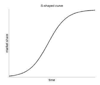
FIGURE 6.1. The S-shaped development curve goes through three stages: an initial stage of exponential growth, a period of steady growth, and finally a period of saturation. This plot shows market share of a hypothetical company as a function of time.

Once again, the future need not resemble the past. In fact, the record of most analysts is not much better than that of chartists. Their predictions routinely fail to beat naïve forecasts, and funds that hold all the stocks in a particular index routinely outperform managed funds, at least after expenses. Some do much better, but the occasional success story may be simple luck: every investment strategy has to win some of the time. As the economist Burton G. Malkiel wrote, “Financial forecasting appears to be a science that makes astrology look respectable.”26

The mediocre performance of most stock pickers seems to confirm the EMH: in an efficient market, stock selection should be a waste of time because the true value of any asset is always reflected in the price. It is impossible to make better forecasts than the market itself, at least on a consistent basis. Price fluctuations are a random walk, so they are inherently unpredictable. According to Fama, “If the analyst has neither better insights nor new information, he may as well forget about fundamental analysis and choose securities by some random selection procedure.”²⁷ Throwing darts at the financial section of the Wall Street Journal is said to work quite well as a stock-picking technique.

Prices of basic commodities such as oil are especially difficult to forecast, because both supply and demand are subject to shifting political, economic, and geographic factors.²⁸ The export quotas of OPEC countries are determined by their oil reserves, so there is an incentive to inflate the estimates. Many of the OPEC nations involved are notoriously unstable (the Middle East), unpredictable (Venezuela), or at risk of terrorism. As much as a fifth of the 2006 oil price is made up of the so-called political-risk premium, which spikes every time there is a perceived threat against an oil supplier or the transport network. Hurricanes are also a factor, as seen by the fluctuations in oil price as the storms duck and weave their way towards Gulf coast refineries.

Even markets that are not that efficient are hard to predict—like real estate, where there are few buyers per property, and the process of buying or selling is relatively slow and expensive. Some housing markets are believed to follow cyclical trends.29 When house prices are at a low level relative to the cost of renting, new buyers enter the market because it is affordable. As prices begin to rise, speculators join the party, driving the price up with positive feedback. When house prices grow too high relative to rents, the supply of first-time buyers is cut off and the market reaches a plateau—negative feedback. If prices begin to fall, more sellers will try to off-load their properties, driving prices down: positive feedback in the other direction. The cycle therefore continues. However, there are many other factors to take into account, and even if such a cycle does exist, the pattern constantly varies. It is hard to know when turning points will occur, and even harder to beat a buy-and-hold strategy once transaction fees are taken into account.

If no individual person can predict the future, perhaps several people can. In 1948, the RAND Corporation came up with a method of making decisions based on an ensemble approach. A number of experts were polled on a series of questions. The questions were refined based on their input, and the process repeated until a group consensus was obtained. The method, known as Delphi after the Greek oracle, was first used by the United States Defense Department to investigate what would happen in a nuclear war, but it was soon adopted by businesses for making financial decisions.

Imagine that you are a theoprope who has time-travelled from ancient Greece. You have heard of this place called Delphi. You show up at an office in a high-rise in downtown New York. You hand the bemused-looking secretary a goat. She shows you to a room. Inside are . . . a group of management consultants. “Hello, Mr.Theopropous,” says one. “We’ve come to a consensus. We will have the Mediterranean lunch special, all round.” You run out screaming. Not only did the new-version Delphi lack a certain mystique, but it wasn’t very good at predicting the future. A 1991 study by the experimental psychologist Fred Woudenberg showed that the Delphi was no more accurate than other decision-making methods, because “consensus is achieved mainly by group pressure to conformity.”³⁰

So if financial analysts of all stripes cannot predict the future, why are there so many of them, and why are they so well reimbursed? Would the market work just as well without them? The fact is that the market augurs exist because they do make a lot of money—for themselves and their employers. Buying and holding may be good for the client, but the fastest way to generate commissions is by buying, selling, buying again, and so on. Also, there is a strong market for predictions, and accuracy is of secondary importance. It is always easy to generate data that makes it look as if a method has been highly reliable in the past. Finally, as discussed below, some stock pickers really do manage to beat the market, at least for a while.

Of course, if all the chartists, analysts, and consultants were replaced with chimps armed with darts, the market would disintegrate pretty rapidly. If the market has any semblance of efficiency, it is because of the combined efforts of predictors who make up the investor ecosystem. You could argue that if the system has parasites, it is those who invest in index funds. These funds tend to purchase the stocks that have been picked by active managers, so investors benefit passively from their decisions.

THE GLOBAL CAPITAL MODEL

Chartists and analysts both focus on particular assets or asset classes. On a grander scale, major private and governmental banks, some economic- forecasting firms, and institutions such as the Organization for Economic Co-operation and Development (OECD) have developed large econometric models that attempt, in the style of Jevons, to simulate the entire economy by aggregating over individuals. Their aim is to make macro-economic forecasts of quantities such as gross domestic product (GDP), which is a measure of total economic output, and to predict recessions and other turning points in the economy, which are of vital interest to companies or governments. The models are similar in principle to those used in weather forecasting or biology, but they involve hundreds or sometimes thousands of economic variables, including tax rates, employment, spending, measures of consumer confidence, and so on.

In these models, like the others, the variables interact in complex ways with multiple feedback loops. An increase in immigration may cause a temporary rise in unemployment, but over time, immigration will grow the economy and create new jobs, so unemployment actually falls. This may attract more immigrants, in a positive feedback loop, or heighten social resistance to immigration from those already there—negative feedback. The net effect depends on a myriad of local details, such as what each immigrant actually does when he arrives. The model equations therefore represent parameterizations of the underlying complex processes, and they attempt to capture correlations between variables, either measured or inferred from theory. Again, the combination of positive and negative feedback loops tends to make the equations sensitive to changes in parameterization. The model is checked by running it against historical data from the past couple of decades and comparing its predictions with actual results. The parameters are then adjusted to improve the performance, and the process is repeated until the model is reasonably consistent with the historical data.

While the model can be adjusted to predict the past quite well—there is no shortage of knobs to adjust—this doesn’t mean that it can predict the future. As an example, the black circles in figure 6.2 show annual growth in GDP for the G7 countries (the United States, Japan, Germany, France, Italy, the United Kingdom, and Canada). The white circles are the OECD forecasts, made a year in advance, and represent a combination of model output and the subjective judgment of the OECD secretariat. The forecast errors, which have standard deviation 0.95, are comparable in magnitude to the fluctuations in what is being forecast, with standard deviation 1.0. The situation is analogous to the naïve “climatology” forecast in weather prediction, where the forecast error is exactly equal to the natural fluctuations of the weather.

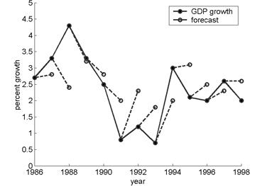
FIGURE 6.2. GDP growth for the G7 countries, plotted against the OECD one-year predictions, for the period 1986 to 1998. Standard deviation of errors is 0.95, that of the GDP growth is 1.0.31

These results are not unique to the OECD, but are typical of the performance of such forecasts, which routinely fail to anticipate turning points in the economy.32 As The Economist noted in 1991, “The failure of virtually every forecaster to predict the recent recessions in America has generated yet more skepticism about the value of economic forecasts.”³³ And again in 2005, “Despite containing hundreds of equations, models are notoriously bad at predicting recessions.”³⁴ In fact, if investors used econometric models to predict the prices of assets and gamble on the stock or currency markets, they would actually lose money.³⁵ Consensus between an ensemble of different models is no guarantor of accuracy: economic models agree with one another far more often than they do with the real economy.³⁶ Nor does increasing the size and complexity of the model make results any better: large models do no better than small ones.³⁷ The reason is that the more parameters used, the harder it is to find their right value. As the physicist Joe McCauley put it, “The models are too complicated and based on too few good ideas and too many unknown parameters to be very useful.”³⁸ Of course, the parameters can be adjusted and epicycles added (just as the ancients did with the Greek Circle Model) until the model agrees with historical data. But the economy’s past is no guide to its future.

Similar models are used to estimate the impact of policy changes such as interest hikes or tax changes—but again, the results are sensitive to the choices of the modeller and are prone to error. In one 1998 study, economist Ross McKitrick ran two simulations of how Canada’s economy would respond to an average tax cut of 2 percent, with subtle differences in parameterization. One implied that the government would have to cut spending by 27.7 percent, while the other implied a cut of only 5.6 percent—a difference of almost a factor five. In the 1990s, models were widely used to assess the economic effects of the North American Free Trade Agreement (NAFTA). A 2005 study by Timothy Kehoe, however, showed that “the models drastically underestimated the impact of NAFTA on North American trade, which has exploded over the past decade.”

In a way, the poor success rate of economic forecasting again seems to confirm the hypothesis that markets are efficient. As Burton Malkiel argued, “The fact that no one, or no technique, can consistently predict the future represents . . . a resounding confirmation of the random-walk approach.”³⁹ It also raises the question why legions of highly paid professionals—including a large proportion of mathematics graduates—are employed to chart the future course of the economy. And why governments and businesses would follow their advice.

RATIONAL ECONOMISTS

Now, a non-economist might read the above and ask, in an objective, rational way, “Can modern economic theory be based on the idea that I, and the people in my immediate family, are rational investors? Ha! What about that piece of land I inherited in a Florida swamp?” Indeed, the EMH sounds like a theory concocted by extremely sober economists whose idea of “irrational behaviour” would be to order an extra scoop of ice cream on their pie at the MIT cafeteria. Much of its appeal, however, lay in the fact that it provided useful tools to assess risk. As Bachelier pointed out, the fact that the markets are unpredictable does not mean that we cannot calculate risks or make wise investments. A roll of the dice is random, but a good gambler can still know the odds. The EMH made possible a whole range of sophisticated probabilistic financial techniques that are still taught and used today. These include the capital asset pricing model, modern portfolio theory, and the Black- Scholes formula for pricing options.

The capital asset pricing model was introduced by the American economist William F. Sharpe in the 1960s as a way to value a financial asset by taking into account factors such as the asset’s risk, as measured by the standard deviation of past price fluctuations. It provides a kind of gold standard for value investors. The aim of modern portfolio theory, developed by Harry Markowitz, was to engineer a portfolio that would control the total amount of risk. It showed that portfolio volatility can be reduced by diversifying into holdings that have little correlation. (In other words, don’t put all your eggs in the same basket, or even similar baskets.) Each security is assigned a number β, which describes its correlation with the market as a whole. A β of 1 implies that the asset fluctuates with the rest of the market, but a β of 2 means its swings tend to be twice as large and a β of 0.5 means it is half as volatile. A portfolio with securities that tend to react in different ways to a given event will result in less overall volatility.

The Black-Scholes method is a clever technique for pricing options (which are financial instruments that allow investors to buy or sell a security for a fixed price at some time in the future). Aristotle’s Politics describes how the philosopher Thales predicted, on the basis of astrology, that the coming harvest would produce a bumper olive crop. He took out an option with the local olive pressers to guarantee the use of their presses at the usual rate. “Then the time of the olive-harvest came, and as there was a sudden and simultaneous demand for oil-presses he hired them out at any price he liked to ask. He made a lot of money, and so demonstrated that it is easy for philosophers to become rich, if they want to; but that is not their object in life.”40 Today, there are a wide variety of financial derivatives that businesses and investors use to reduce risk or make a profit. Despite the fact that options have been around a long time, it seems that no one, even philosophers, really knew how to price them until Black-Scholes. So that was a good thing.

All of these methods were built on the foundations of the EMH, so they treated investors as inert and rational “profit-maxi-mizers,” modelled price fluctuations with the bell curve, and reduced the measurement of risk to simple parameters like volatility. There were some objections to this rather sterile vision of the economy. Volatility of assets seemed to be larger than expected from the EMH.41 Some psychologists even made the point that not all investors are rational, and they are often influenced by what other investors are doing. As Keynes had argued in the 1930s, events such as the Great Depression or the South Sea Bubble could be attributed to alternating waves of elation or depression on the part of investors. The homme moyen, it was rumoured, was subject to wild mood swings.

On the whole, though, the EMH seemed to put economic theory on some kind of logical footing, and it enabled economists to price options and quantify risk in a way that previously hadn’t been possible. The “model” for predicting an asset’s correct value was just the price as set by the market, and it was always perfect. Even if all investors were not 100 percent rational, the new computer systems that had been set up to manage large portfolios had none of their psychological issues. Perhaps for the first time, market movements could be understood and risk contained. To many economists, the assumptions behind the orthodox theory seemed reasonable, at least until October 19, 1987.

COMPLICATIONS

According to random walk theory, market fluctuations are like a toss of the die in a casino. On Black Monday, the homme moyen, Mr. Average, sat down at a craps table. The only shooter, he tossed two sixes, a loss. Then two more, and two more. Beginning to enjoy himself in a perverse kind of way—nothing so out of the normal had happened to him in his life—he tried several more rolls, each one a pair of sixes. People started to gather around and bet that his shooting streak would not continue. Surveillance cameras in the casino swivelled around to monitor the table. The sixes kept coming. Soon, the average man was a star, a shooting star flaming out in a steady stream of sixes and taking everyone with him. At the end of the evening, when security guards pried the die out of his fingers, he had rolled thirty twelves in a row and was ready for more. The net worth of everyone in the room who bet against his streak had decreased, on average, by 29.2 percent. Someone in the house did the math and figured out the odds of that happening were one in about ten followed by forty-five zeros—math-speak for impossible.

Black Monday, when the Dow Jones index fell by just that amount, was an equally unlikely event—and a huge wakeup call to the economics establishment. According to the EMH, which assumes that market events follow a normal distribution, it simply shouldn’t have happened. Some have theorized that it was triggered by automatic computer orders, which created a cascade of selling. Yet this didn’t explain why world markets that did not have automatic sell orders also fell sharply. Unlike the South Sea Bubble, which was at least partly rooted in fraud, Black Monday came out of nowhere and spread around the world like a contagious disease. It was as if the stock market suddenly just broke. But it has been followed by a string of similar crashes, including one in 1998 that reduced the value of East Asian stock markets by $2 trillion, and the collapse of the Internet bubble. Perhaps markets aren’t so efficient or rational after all.

A strong critic of efficient-market theory has been Warren Buffet, who in 1988 observed that despite events such as Black Monday, most economists seemed set on defending the EMH at all costs: “Apparently, a reluctance to recant, and thereby to demystify the priesthood, is not limited to theologians.” Another critic was an early supporter (and Eugene Fama’s ex-supervisor), the mathematician Benoit Mandelbrot. He is best known for his work in fractals (a name he derived from the Latin fractus, for “broken”). Fractal geometry is a geometry of crooked lines that twist and weave in unpredictable ways. Mandelbrot turned the tools of fractal analysis to economic time series. Rather than being a random walk, with each change following a normal distribution, they turned out to have some intriguing features. They had the property, common to fractal systems, of being self-similar over different scales: a plot of the market movements had a similar appearance whether viewed over time periods of days or years (see boxed text below). They also had a kind of memory. A large change one day increased the chance of a large change the next, and long stretches where little happened would be followed by bursts of intense volatility. The markets were not like a calm sea, with a constant succession of “normal” waves, but like an unpredictable ocean with many violent storms lurking over the horizon.

BORDERLINE NORMAL

Lewis Fry Richardson, the inventor of numerical weather forecasting, once did an experiment in which he compared the lengths of borders between countries, as measured by each country. For example, Portugal believed its border with Spain was 1,214 kilometres long, but Spain thought it was only 987 kilometres. The problem was that the border was not a straight line, so the length would depend on the scale of the map used to measure it. A large scale includes all the zigs and zags, while a small scale misses these and give a shorter result. If the measured length is plotted as a function of the scale, it turns out to follow a simple pattern known as a power law. In a 1967 paper, Benoit Mandelbrot showed how this could be used to define the border’s fractal dimension, which was a measure of its roughness.

If the border was a one-dimensional straight line, its length on the map would vary linearly with the scale—a map with twice the scale would show everything twice as long, including the border. The area of a two-dimensional object such as a circle would vary with the scale to the power of two—double the scale and the area increases by a factor of four. If the length of a border increases with scale to the power D, then D plays the role of dimension. Mandelbrot showed that the British coastline has a fractal dimension D of about 1.25.

Like clouds, fractal systems reveal a similar amount of detail over a large range of scales. There is no unique “normal,” or correct, scale by which to measure them. Similarly, the fluctuations of an asset or market show fractal-like structure over different time scales, which makes analysis using orthodox techniques difficult.

In the 1990s, researchers tested the orthodox theory by poring over scads of financial data from around the world. The theory assumes, for example, that a security has a certain volatility, and that it varies in a fixed way with other assets and the rest of the market. The volatility can in principle be found by plotting the asset’s price changes and calculating the standard deviation. In reality, though, the actual distributions have so-called fat tails, which means that extreme events—those in the tails of the distribution—occur much more frequently than they should. One consequence is that the volatility changes with time.42 An asset’s correlation with the rest of the market is also not well defined. It is always possible to plot two data sets against each other and draw a straight line through the resulting cloud of points, as Galton did for his height measurements. But economic data is often so noisy that the slope of the line says little about any underlying connection between sets.⁴³

Perhaps the biggest problem with the orthodox economic theory, though, is its use of the bell curve to describe variation in financial quantities. When scientists try to model a complex system, they begin by looking for symmetric, invariant principles: the circles and squares of classical geometry; Newton’s law of gravity. Einstein developed his theory of relativity by arguing that the laws of physics should remain invariant under a change of reference frame. The normal distribution has the same kind of properties. It is symmetric around the mean, and is invariant both to basic mathematical operations and to small changes to the sample. If the heights of men and women each follow a bell curve, then the mid-heights of couples will be another bell curve, as in figure 5.1 (see page 178). Adding a few more couples to the sample should not drastically change the average or standard deviation.

The normal distribution means that volatility, risk, or variation of any kind can be expressed as a single number (the standard deviation), just as a circle can be described by its radius or a square by the length of one side. However, the empirical fact that asset volatility changes with time indicates that this is an oversimplification. The bell curve can be mathematically justified only if each event that contributes to fluctuation is independent and identically distributed. But fluctuations in the marketplace are caused by the decisions of individual investors, who are part of a social network. Investors are not independent or identical, and therefore they cannot be assumed to be “normal.” And as a result, neither can the market. Indeed, it turns out that much of the data of interest is better represented by a rather different distribution, known as a power-law distribution.

POWER TO THE PEOPLE

Suppose there existed a country in which the size of its cities was normally distributed, with an average size of half a million. Most people would live in a city that was close to the average. The chances of any city being either smaller or larger than average would be roughly the same, and none would be extremely large or extremely small. The expressions “small town” and “big city” would refer only to subtle variations. The pattern in real countries is quite different. One 1997 study tabulated the sizes of the 2,400 largest cities in the United States. The study’s authors found that the number of cities of a particular size varies inversely with the size squared (to the power of two). This so-called power-law pattern continues from the largest city, New York, right down to towns of only 10,000 residents.44 This distribution is highly asymmetrical. For each city with a certain population, there are, on average, four cities of half the size, but only a quarter the number of cities twice the size—so there are many more small towns than would be predicted from a normal distribution. The distribution is fat-tailed—the largest metropolis, New York, is far bigger than the mean. Even the home of Wall Street, it seems, is not normal. The same pattern was found for the 2,700 largest cities in the world.

A similar asymmetrical distribution—sometimes known as Pareto’s law, after the nineteenth-century Italian who first discovered it—holds for personal wealth. Perhaps Warren Buffet so distrusted the EMH because if the normal distribution were correct, he shouldn’t exist. Most people would enjoy a uniform degree of financial success; no one would be extremely poor or exceptionally rich. In reality, however, the wealthy are arranged like cities. For every millionaire in the United States, there are about four people with half a million, sixteen with a quarter million, and so on. If heights were arranged in a similar way, then most people would be midgets, but a small number would be giants.

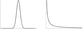
FIGURE 6.3. The left panel shows a normal distribution, the right a power-law distribution. The horizontal axis could, for example, represent wealth or city size. In reality, the power-law distribution holds only over a certain range, so there are cutoffs in both the vertical and the horizontal axes. In the normal distribution, it is possible to assume that most samples are close to the mean. In a power-law distribution, we cannot ignore the samples in the extreme right-hand tail (because they are the most important in terms of the quantity measured) or those in the left (because there are so many of them).

The growth of an investor’s assets, or a city’s population, is not a completely random event, but depends on its position in a connected network.45 A person thinking to move is more likely to know people or employers in a large town than in a small town. Big cities draw people to them like moths. Money attracts more money; the rich get richer; strong countries attract investment, while those on the periphery remain vulnerable. The economy consists of both negative feedback loops, like Adam Smith’s invisible hand, and positive feedback loops, which amplify differences. In such situations, Galton’s principle of “regression to the mean” is highly misleading. What goes up needn’t come down.

Imagine that several different restaurants of similar quality start business on the same day, and that, for some random reason, one restaurant initially attracts a few more customers than the others. (Perhaps its location is slightly better, or the proprietor is well known and popular.) A visitor who lacks detailed information will likely choose the restaurant that holds a few more people, just because that implies that it must be reasonably good. Therefore, the number of customers is amplified by positive feedback: the more customers there are, the more new ones will be generated. As business improves, the proprietor may invest the proceeds in better ingredients (product quality), in advertising (brand equity), or in expanding the restaurant (economies of scale). The restaurant pulls further ahead of its competition. Growth may eventually saturate—when, for example, some of the customers grow bored with the menu. The company therefore follows the S-shaped curve of figure 6.1 (see page 237). Meanwhile, the restaurant down the road, which was just as good to start off with, quietly goes bust within a year or two—as most new businesses do. Positive feedback amplifies changes, be they good or bad, so it can lead to collapse as well as growth.

The power-law distribution holds, in an approximate fashion, over many different phenomena, from the size of earthquakes to the number of interactions in a biological network (like that in figure 5.4 on page 203).⁴⁶ Unfortunately, this does not help much with prediction of particular events, because it implies that there is no typical representative. It is no longer possible to predict that an individual sample will be close to the mean, give or take a standard deviation or two. Even the calculation of the mean depends critically on the sample. It has been estimated that if Bill Gates attends a baseball game at Safeco Field in Seattle, the average net worth of those also in attendance increases by a factor of four.⁴⁷ Leave him out of the calculation, and you miss the most important person. There is no easy mathematical shortcut. Details matter, and nothing is “normal.”

Like customers choosing a restaurant, investors must be viewed as individual but interdependent agents operating in a highly connected network. The decisions they make can ripple through the entire system. Any accurate model of the economy would have to take into account these intricate social dynamics, which are explicitly ignored by the EMH. Despite these drawbacks, no serious alternative is close to dislodging the orthodox theory from the throne of predictive economics. So why is this the case? And is there anything better available?

STICKY THEORY

The orthodox economic theory has proved so resilient because it is both hard to beat—in the sense that other equations do little better at predicting the future or estimating risk—and highly adaptable. More elaborate versions of the basic theory attempt to correct the flaws while retaining the same structure. The field of behavioural economics, for example, addresses psychological effects such as loss aversion. Owners of financial assets hate to sell at a lower price than they paid, so they resist selling after a downturn. Therefore, prices tend to be “sticky” on the way down. Models can be tweaked and adjusted to accommodate these behavioural effects, by incorporating parameterizations of investor psychology, which still treat each investor as having fixed tastes and preferences. These adjustments relax the condition of investor rationality but still assume that investors can be modelled rationally. They therefore do not address the underlying problem, which is that the economy is a social process that cannot be reduced to law.48

Another approach is to stretch the theory so it better allows for extreme events. Consider, for example, the Mexican peso crisis of 1994–95. The standard deviation of the peso-dollar exchange rate from November 19, 1993, to December 16, 1994, was 0.47 percent. According to random walk theory, someone buying pesos on December 19, 1994, should have expected to lose no more than 3.5 percent of his dollar investment over a two-week period, ninety-nine times out of a hundred. As it turns out, losses were 65 percent, which in principle should not have happened in a billion years.⁴⁹ The reasons behind the high losses—a peasant uprising in Chiapas and the death of a presidential candidate—were local to Mexico. But the crisis was soon followed by sister crises around the world: the collapse of Asian currencies (1997–98) and Russian bonds (1998).

To account for such sudden changes in volatility, more sophisticated risk-assessment techniques have been developed, such as the generalized autoregressive conditional heteroskedasticity (GARCH).⁵⁰ The last word, to you and me, means changing variability; autoregressive means that the changes depend on past behaviour. In its most basic form, GARCH produces a distribution of price changes that better accounts for extreme events, but at the expense of two new parameters. These add to the number of unknowns, as well as the number of Greek letters in the equations, and still cannot begin to account for the inherently social and political nature of the market (there is no parameter for peasant uprising). As Mandelbrot put it, “The high priests of modern financial theory keep moving the target. As each anomaly is reported, a ‘fix’ is made to accommodate it. . . . But such ad hoc fixes are medieval. They are akin to the countless adjustments that defenders of the old Ptolemaic cosmology made to accommodate pesky new astronomical observations.” ⁵¹ In practice, it seems hard to find numerical techniques that improve greatly on the orthodox methods, which is why they are still orthodox. Forecasters can always try to get around shortcomings in the model output by applying their subjective judgment. One currency trader said that pricing techniques such as Black-Scholes only represent the numerical approach to the problem: “Although used as a first cut, the actual price quoted takes non-quantitative factors into account.”⁵²

Another reason for the theory’s endurance is the lock-in effect: it has become entrenched in academic circles and elsewhere. Just as the perfect model hypothesis in weather forecasting enables researchers to do complicated, pseudo-probabilistic analyses of the atmosphere, so orthodox theory allows the development of intimidating and authoritative financial techniques. As the economist Paul Ormerod wrote, “Maximizing behaviour, for all its faults, is a valuable security blanket for many economists. It enables the mathematics of differential calculus to be applied to their theories, and for some intellectually satisfying results to be obtained. It has the side-benefit, too, of inducing mortal terror in many scholars from other disciplines in the social sciences who lack the required amount of mathematical training.”⁵³ This is reminiscent of Iamblichus’s statement about the Pythagoreans: “Their writings and all the books which they published were not composed in a popular and vulgar diction, so as to be immediately understood, but in such a way as to conceal, after an arcane mode, divine mysteries from the uninitiated.”⁵⁴

One defence of the orthodox theory is that it correctly predicts that the market is unpredictable. If, it is argued, the market is irrational, then a rational investor would be able to consistently outsmart it.⁵⁵ But while an efficient market implies unpredictability, the opposite is not true. It is actually rather strange that unpredictability is cited as evidence of logical calm. A drunken man’s stumbling (the original inspiration for the random walk) might be unpredictable, but we wouldn’t call his behaviour hyper-rational.

Perhaps the greatest attraction of orthodox theory lies in its subtext. It allows economists to maintain the illusion that the economy is fundamentally rational, and that their models are correct. The causes of error are externalized to random external shocks. The tenets of the theory—that investors are independent and fixed in their tastes, and can look into the future to calculate value—reflect the Pythagorean ideals of an ordered universe. They are also exactly the assumptions that need to be made if economic models are to be considered accurate and economists are to maintain any oracular authority. As soon as we admit that the economy is a complex set of interactions in a huge connected network, and that it involves individuals whose “beliefs, interpretations and justifications evolve and transform themselves continuously,” then the idea of accurate mathematical models begins to seem, to paraphrase Immanuel Kant, a little absurd. The system is uncomputable, and there is no Apollo’s arrow to fly into its future. It is interesting that Bachelier, whose work was at first spurned, was not allowed back in the fold until his random walk hypothesis was reconciled with this image of a rational marketplace.

Indeed, a huge amount of effort has gone into explaining rationally why the market is rational. This leads to the kind of double- think that allowed astronomers to retain the notion of perfectly circular motion, despite much evidence to the contrary, for about 2,000 years.⁵⁶ Another example of double-think occurred during the summer of 1988, when a severe drought in the United States Midwest affected the supply of corn and soybeans. As time went on and the drought continued, prices of these commodities rose to extreme heights. Then one day, Chicago experienced a tiny, insignificant amount of rain—one imagines a few drops sprinkled on the balding pate of a broker as he headed out to work in the morning— and prices collapsed. Some saw this as a sign that markets might be a touch on the manic, oversensitive side, but efficient-market enthusiasts disagreed. One top economist insisted that the response in the market was quite rational, because investors know that weather tends to be persistent, so they all updated their forecasts with this new information and concluded that the drought would not continue. ⁵⁷ Given the uncertainty in weather forecasts of any type, it seems to be stretching the meaning of the word “rational” to allow a few rain clouds to so drastically change expectations for the future.

THE PSYCHOLOGY OF ECONOMICS

Here are some factors that behavioural psychologists believe affect investors:
Compartmentalizing.Investors divide problems into parts and treat each separately, instead of looking at the big picture. Losing ten dollars on the street feels worse than losing the same amount in a stock portfolio because each event is handled in a different mental compartment.
Trend following.Extrapolating from current conditions tends to fuel bubbles because when the market is going down, people expect it to stay down, and when it is going up, the sky is the limit.
Loss aversion.People take less pleasure in winning ten dollars than they do pain in losing the same amount. A consequence is that investors will avoid selling assets at a loss.
Denial.Investors maintain beliefs even if they are at odds with the evidence. This results in cognitive dissonance.
Suggestion.They are overly influenced by the opinions of others.
Status quo bias.They tend to avoid change. It means that transactions, which always involve some kind of change, have a hidden extra cost.
Illusory correlations.Investors look for patterns where they don’t exist. This is also called superstition.

Interestingly, such psychological effects—denial, the power of suggestion, status quo bias, and fear of loss—may also explain why human beings cling to their predictive models even when the results don’t agree with reality.

INVESTMENT STORIES

Of course not all economists, and certainly not all traders, agree with the hypothesis that the market is without even pockets of predictability. People such as the former hedge fund manager George Soros do quite well by following their intuitive feel for market sentiment, and betting against trends. It is interesting to compare the EMH vision of rational investors with Soros’s notion of “radical fallibility,” which contends that “all the constructs of the human mind . . . are deficient in one way or another.”58 (This includes investment ideas or stories—such as South Sea gold, Internet stocks, and indeed abstract economic theories like the EMH—which grow and reinforce themselves in a positive feedback loop as they become established in the investment community.) Profit opportunities arise when you can spot the flaw in the story and bet against it. Because the market is constantly changing and adapting, investment strategies and mental models are themselves nothing but “fertile fallacies” that must be fixed or discarded when they no longer work.

The dangers of excessive confidence in models were amply illustrated by the 1998 collapse of Long-Term Capital Management LP. This hedge fund had a number of economics luminaries on its ticket, including Myron Scholes (of the Black-Scholes formula). It used efficient-market theory to construct complicated and highly leveraged financial bets, which worked well until August 1998, when the Russian government decided to throw efficiency to the winds and default on its bonds. The subsequent market collapse, unanticipated by the equations, meant that to avoid an even greater crisis, the firm had to be rescued in a $3.6-billion bailout.

Attempts are still made to develop investment techniques based on quantitative, predictive models, but they tend to be data-driven rather than model-driven. These can involve classical statistical techniques, which search for correlations in data, or biology-inspired techniques involving neural networks and genetic algorithms. The first biology-inspired approach simulates the way that the brain works by setting up a network of artificial “neurons” that learn to detect patterns in streams of financial data. The latter approach sets alternative algorithms into competition, then chooses the winner in a process akin to natural selection. The aim is not to simulate the underlying economy, but to seek trends in the financial data itself. Such methods may analyze anything at all—say, the dollar-sterling exchange rate and the price of pork bellies—to detect patterns that (for good reason) elude most investors. In the world of finance, even a tiny advantage can lead to substantial profits—at least if you are backed by a large bank, so that positions can be heavily leveraged and transaction costs controlled. The Prediction Company, set up by physicists and funded by the Swiss bank UBS AG, is one firm which uses such techniques.⁵⁹ It is hard to judge the firm’s success in the somewhat opaque world of financial prediction, but it is still around after more than fifteen years.

Ultimately, though, all such models, like those of the chartist, depend on the future’s resembling the past. They seem more alchemy than science. One trader at a major New York investment firm, which employs a large team of about a hundred “quants,” or quantitative analysts, told me that it was a “matter of debate” within the firm whether research into predictive mathematical models, beyond simple valuation tools, was worthwhile for them. This is also why the chairman of the U.S. Federal Reserve has yet to be replaced by a machine. The market is a social process that deals in fictions as well as reality, words as well as numbers. Mathematical models certainly have their uses, but they only give part of the story and can be misleading if taken out of context. In the markets, number is not all. Just as computers are not good at spotting social trends or interpreting stories, they do not seem brilliant at making market predictions. For most investors, the teachings of the EMH are quite useful— diversify among different asset classes, avoid expensive management fees, and be wary of prophets who claim to foretell the future. To which could be added: risks may be larger than they appear.

THE LIVING ECONOMY

Even if models are not predictive, they can still be used to capture aspects of the economy’s dynamics in a more realistic way. Models have been produced of a hypothetical stock market, for example, in which individual agents are assumed to have their own preferred investment strategy.60 Some will tend to follow the current psychology and accentuate market swings (positive feedback), while others base their decisions on value analysis and go against trend when they feel the market is too high or too low (negative feedback). The price at any time represents a dynamic balance between these forces: subjective greed or panic versus “objective” calculations of value. The behaviour gets interesting when the market participants are allowed to influence one another: if a majority thinks that the market is going to tank, then this mood eventually deflates the most optimistic chart-follower. Predictions therefore affect the future in a self-reinforcing, positive feedback loop. Tastes and preferences are treated as dynamic rather than fixed. The result is an inherently unstable system that mimics typical market behaviour, including booms and busts. There is no invisible hand to guide it to equilibrium; no such equilibrium even exists.

Agent-based models are an interesting area of research activity, and they can yield insight into the underlying dynamics of markets, as well as expose flaws in the orthodox theory. They can also be used to do “what if ” simulations for particular situations—for example, to see how a change in a company’s transportation network might affect delivery times. However, it is questionable whether they can help to make more general predictions. It is one thing to produce market-like behaviour in an abstract system, another to forecast what will happen in the real market.⁶¹

One phenomenon poorly explained by orthodox economic theory is the apparent excess volatility of financial assets, which is inconsistent with the hypothesis that volatility is caused purely by external shocks. Comparisons with biological systems suggest reasons why this is the case. The metabolism of a cell is controlled by many different proteins. The number of molecules of each protein varies in a random way, owing to stochastic effects. The cell also misreads cues from the environment. The resulting variation can be interpreted as a kind of prediction error: the cell produces too many of some proteins and not enough of another, and it also reacts to its own errors. The result is that even in the absence of external shocks, the rate of metabolism will fluctuate randomly. Organisms, like the yeast in Chapter 5, have evolved complex feedback loops that reduce but do not eliminate this natural variation.

Similarly, an economy can be seen as a kind of super-organism and its output a measure of metabolism. The economy takes in resources from people and the environment, transfers them into material wealth, and expels waste products. Value circulates through the economy, changing form from matter to money to labour in a ceaseless flow. The net output is controlled by a large number of individuals and companies, each of which is constantly adjusting output in accord with its predictions about the future. Because the predictions are erroneous, control is incomplete, and the response of each actor is inherently creative, net output will fluctuate randomly of its own accord, adding to volatility.⁶² The market is therefore not a dead thing, at equilibrium; as traders like to say, it has a life of its own.

Just as biological systems dislike excess volatility and incorporate complex feedback loops to reduce it, sophisticated economies develop mechanisms to damp out volatile fluctuations. An example is insurance. Let’s say a disaster such as a crop-destroying drought has driven individual farmers, whose weather predictions were wrong, into bankruptcy. This has knock-on effects on the rest of the economy, which amplifies the disaster’s impact through positive feedback. But with insurance, the loss is dissipated through financial structures that are less vulnerable to collapse than an individual farmer—negative feedback. Similarly, tools such as options or futures contracts allow businesses to smooth out fluctuations in prices and increase their own value. These effects can be simulated (but not precisely predicted) using simple top-down models that capture overall function.

The biological analogy suggests that while the orthodox theory is right to state that the market is practically impossible to predict, it is right for the wrong reasons. The EMH assumes that market fluctuations are the result of random external shocks, and that its response is governed by rational laws. In other words, it treats the economy as a dead object that can be modelled like a falling stone. However, a model that views the economy as a kind of super-organism would ascribe fluctuations not just to external causes but to the market itself. What makes its response unpredictable is to a large part its own inability to predict. And like a living organism, the economy represents a shifting, dynamic balance between opposing forces—positive and negative feedback loops, buyers and sellers— so models are sensitive to changes in parameterization.

In its insistence on rationality, the EMH is therefore a strange inversion of reality. Its primary aim, it appears, is not to predict the future, but to make it look like we all know what we’re doing. This is dangerous for two reasons. The first is that because the EMH views the market as “normal,” it gives an illusion of control, and at the same time it tends to underestimate the real risk of future financial storms. This is especially a concern when the results are incorporated in policy. As the economist Kenneth Arrow, who worked as a weather forecaster during the Second World War, put it: “Vast ills have followed a belief in certainty, whether historical inevitability, grand diplomatic designs, or extreme views on economic policy. When developing policy with wide effects for an individual or society, caution is needed because we cannot predict the consequences.”63 There is a curious disconnect between the consistent inaccuracy of the forecasts and the confidence with which politicians, banks, and business leaders regularly use them to make important decisions. The second danger comes from the insidious idea that “the market is always right,” that it is some kind of hyper-rational being that can outwit any speculator or government regulator. This view of the economy, enshrined in the EMH, turns the market into a deity who is watched over, granted legitimacy, and explained to the rest of us by the economic priesthood. It leads to what George Soros has described as a “market fundamentalism,” which is as dangerous as any other kind of fundamentalism and gives a kind of carte blanche to empathy-free corporations to do what they want, under the pretext that they are just being efficient.⁶⁴ People or countries that fail under this system have been judged by the market. But the market is no more rational than the square root of two. It is just the net effect of our own stumbling as we try to find our way in an unpredictable universe.

THREE SIBLINGS

As we’ve seen in these last three chapters, the scientific approaches to making predictions in the areas of weather, health, and wealth share much in common. Atmospheric and economic forecasts have always been linked, even more so when agriculture played a larger part in the economy. This was acknowledged by the Victorian scientist Stanley Jevons when he attempted to predict the business cycle by monitoring sunspots. Francis Galton used his statistical methods to study inheritance, but they have proved equally useful— and much less controversial—in economics. Today, the techniques used by scientists are essentially the same in all three areas, and all have their roots in nineteenth-century astronomy.

While celestial objects are happy to obey dictates like the law of gravity, and are amenable to modelling by equations, systems like the weather and the economy appear more anarchic. The rules they obey are local and social in nature, rather than global. As a result, in all three areas of prediction, scientists run into the same problems. The underlying system is uncomputable, so models rely on parameterizations that introduce model errors. As the model is refined, the number of unknown parameters increases. The multiple feedback loops that characterize such models also make them sensitive to even small errors in parameterization. As a result, the models are highly flexible and can be made to match past data, but accurate predictions of the future remain elusive. The models are often most useful as tools for understanding the present function of the underlying systems.

The three areas of scientific forecasting—weather, health, and wealth—are like siblings. They have the same origins, grew up together, and hung out with some of the same people. Each has its own character. Weather, the eldest, is the one the others look up to, because it is closest to the stars and knows physics. Health, the youngest, used to get in trouble, but it’s flush with optimism as it prepares to come of age. (In its school yearbook, it was voted most likely to find a cure for cancer.) Wealth is the narcissist, spending its days preening in front of the mirror, in thrall to its own beauty and efficiency. In the final part of the book, we find out how these would-be clairvoyants fare as they join forces to take on the greatest challenge of all—a long-term prediction for the planet.