Chapter 2

Working with Data-Analysis Tools

IN THIS CHAPTER

Creating basic and two-input data tables

Analyzing your data using the Goal Seek tool

Creating and running scenarios

Optimizing your data with the Solver tool

When it comes to data analysis, you're best off getting Excel to perform most — or, ideally, all — of the work. After all, Excel is a complex, powerful, and expensive piece of software, so why shouldn’t it take on the lion’s share of the data-analysis chores? Sure, you still have to get your data into the worksheet (although a bit later in the book, I talk about ways to get Excel to help with that chore, too), but after you’ve done that, it’s time for Excel to get busy.

In this chapter, you investigate some built-in Excel tools that will handle most of the data analysis dirty work. I show you how to build two different types of data tables; give you the details on using the very cool Goal Seek tool; delve into scenarios and how to use them for fun and profit; and take you on a tour of the powerful Solver add-in.

Working with Data Tables

If you want to study the effect that different input values have on a formula, one solution is to set up the worksheet model and then manually change the formula’s input cells. For example, if you’re calculating a loan payment, you can enter different interest rate values to see what effect changing the value has on the payment.

The problem with modifying the values of a formula input is that you see only a single result at one time. A better solution is to set up a data table, which is a range that consists of the formula you’re using and multiple input values for that formula. Excel automatically creates a solution to the formula for each different input value.

Data tables are an example of what-if analysis, which is perhaps the most basic method for analyzing worksheet data. With what-if analysis, you first calculate a formula D, based on the input from variables A, B, and C. You then say, “What happens to the result if I change the value of variable A?” “What happens if I change B or C?” and so on.

Don’t confuse data tables with the Excel tables that I talk about in Chapter 3. Remember that a data table is a special range that Excel uses to calculate multiple solutions to a formula.

Creating a basic data table

The most basic type of data table is one that varies only one of the formula’s input cells. Not even remotely surprisingly, this basic version is known far and wide as a one-input data table. Here are the steps to follow to create a one-input data table:

1. Type the input values.
   • To enter the values in a column, start the column one cell down and one cell to the left of the cell containing the formula, as shown in Figure 2-1.
   • To enter the values in a row, start the row one cell up and one cell to the right of the cell containing the formula.
2. Select the range that includes the input values and the formula.
3. Choose Data ⇒ What-If Analysis ⇒ Data Table to open the Data Table dialog box.

4. Enter the address of the input cell, which is the cell referenced by the formula that you want the data table to vary.

   That is, for whatever cell you specify, the data table will substitute each of its input values into that cell and calculate the formula result. You have two choices:

   • If the input values are in a column, enter the input cell’s address in the Column Input Cell text box. In the example shown in Figure 2-1, the data table’s input values are annual interest rates, so the column input cell is C2, as shown in Figure 2-2.
   • If you entered the input values in a row, enter the input cell’s address in the Row Input Cell text box.

5. Click OK.

   Excel fills the input table with the results. Figure 2-3 shows the results of the example data table.

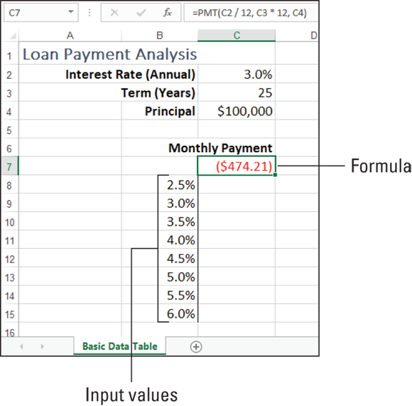
FIGURE 2-1: This data table has the input values in a column.

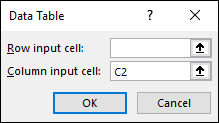
FIGURE 2-2: Enter the address of the input cell.

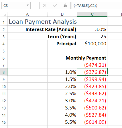
FIGURE 2-3: The data table results.

When you see the data table results, you might find that all the calculated values are identical. What gives? The problem most likely is Excel’s current calculation mode. Choose Formulas ⇒ Calculation Options ⇒ Automatic, and the data table results should recalculate to the correct values.

Creating a two-input data table

Rather than vary a single formula input at a time — as in the one-input data table I discuss in the previous section — Excel also lets you kick things up a notch by enabling you to set up a two-input data table. As you might have guessed, a two-input data table is one that varies two formula inputs at the same time. For example, in a loan payment worksheet, you could set up a two-input data table that varies both the interest rate and the term.

To set up a two-input data table, you must set up two ranges of input cells. One range must appear in a column directly below the formula, and the other range must appear in a row directly to the right of the formula. Here are the steps to follow:

1. Type the input values:

   • To enter the column values, start the column one cell down and one cell to the left of the cell containing the formula.
   • To enter the row values, start the row one cell up and one cell to the right of the cell containing the formula.

   Figure 2-4 shows an example.

2. Select the range that includes the input values and the formula.
3. Choose Data ⇒ What-If Analysis ⇒ Data Table to open the Data Table dialog box.

4. In the Row Input Cell text box, enter the cell address of the input cell that corresponds to the row values you entered.

   In the example shown in Figure 2-4, the row values are term inputs, so the input cell is C3 (see Figure 2-5).

5. In the Column Input Cell text box, enter the cell address of the input cell you want to use for the column values.

   In the example shown in Figure 2-4, the column values are interest rate inputs, so the input cell is C2 (see Figure 2-5).

6. Click OK.

   Excel displays the results. Figure 2-6 shows the results of the example two-input data table.

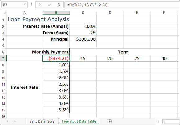
FIGURE 2-4: For a two-input data table, enter one set of values in a column and the other in a row.

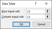
FIGURE 2-5: Enter the addresses of the input cells.

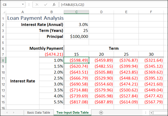
FIGURE 2-6: The two-input data table results.

When you run the Data Table command, Excel enters an array formula in the interior of the data table. The formula is a TABLE function (a special function available only by using the Data Table command) with the following syntax:

{=TABLE(row_input_ref, column_input_ref)}

Here, row_input_ref and column_input_ref are the cell references you entered in the Data Table dialog box. The braces ({ }) indicate an array, which means that you can’t change or delete individual elements within the results. If you want to change the results, you need to select the entire data table and then run the Data Table command again. If you want to delete the results, you must select the entire array and then delete it.

Skipping data tables when calculating workbooks

Because a data table is an array, Excel treats it as a unit, so a worksheet recalculation means that the entire data table is always recalculated. Such a recalculation is not a big problem for a small data table that has just a few dozen formulas. However, it’s not uncommon to have data tables with hundreds or even thousands of formulas, and these larger data tables can really slow down worksheet recalculation.

If you’re working with a large data table, you can reduce the time it takes for Excel to recalculate the workbook if you configure Excel to bypass data tables when it’s running the recalculation. Here are the two methods you can use:

• Choose Formulas ⇒ Calculation Options ⇒ Automatic Except for Data Tables.
• Choose File ⇒ Options to open the Excel Options dialog box, choose Formulas, select the Automatic Except for Data Tables option, and then click OK.

The next time you calculate a workbook, Excel bypasses the data tables.

When you want to recalculate a data table, you can repeat either of the preceding procedures and then choose the Automatic option. On the other hand, if you prefer to leave the Automatic Except for Data Tables option selected, you can still recalculate the data table by selecting any cell inside the data table and either choosing Formulas ⇒ Calculate Now or pressing F9.

Analyzing Data with Goal Seek

What if you already know the formula result you need and you want to produce that result by tweaking one of the formula’s input values? For example, suppose that you know that you need to have $100,000 saved for your children’s college education. In other words, you want to start an investment now that will be worth $100,000 at some point in the future.

This is called a future value calculation, and it requires three parameters:

• The term of the investment
• The interest rate you earn on the investment
• The amount of money you invest each year

Assume that you need that money 18 years from now and that you can make a four percent annual return on your investment. Here’s the question that remains: How much should you invest each year to make your goal?

Sure, you could waste large chunks of your life guessing the answer. Fortunately, you don’t have to, because you can put Excel’s Goal Seek tool to work. Goal Seek works by trying dozens of possibilities — called iterations — that enable it to get closer and closer to a solution. When Goal Seek finds a solution (or finds a solution that’s as close as it can get), it stops and shows you the result.

You must do three things to set up your worksheet for Goal Seek:

• Set up one cell as the changing cell, which is the formula input cell value that Goal Seek will manipulate to reach the goal. In the college fund example, the formula cell that holds the annual deposit is the changing cell.
• Set up the other input values for the formula and give them proper initial values. In the college fund example, you enter four percent for the interest rate and 18 years for the term.
• Create a formula for Goal Seek to use to reach the goal. In the college fund example, you use the FV() function, which calculates the future value of an investment given an interest rate, term, and regular deposit.

When your worksheet is ready for action, here are the steps to follow to get Goal Seek on the job:

1. Select Data ⇒ What-If Analysis ⇒ Goal Seek.

   The Goal Seek dialog box appears.

2. In the Set Cell box, enter the address of the cell that contains the formula you want Goal Seek to work with.
3. In the To Value text box, enter the value that you want Goal Seek to find.

4. In the By Changing Cell box, enter the address of the cell that you want Goal Seek to modify.

   Figure 2-7 shows an example model for the college fund calculation as well as the completed Goal Seek dialog box.

5. Click OK.

   Goal Seek adjusts the changing cell value until it reaches a solution. When it’s done, the formula shows the value you entered in Step 3, as shown in Figure 2-8.

6. Click OK to accept the solution.

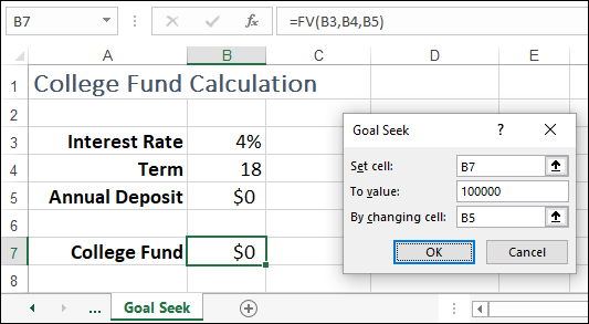
FIGURE 2-7: Using Goal Seek to calculate the annual deposit required to end up with $100,000 in a college fund.

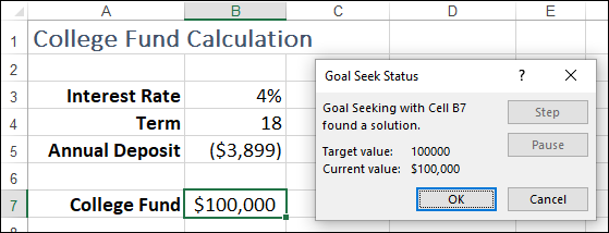
FIGURE 2-8: Goal Seek took all of a second or two to find a solution.

In some cases, Goal Seek might not find an exact solution to your model. Failing to find a solution can happen if Goal Seek takes a relatively long time to find a solution, because Goal Seek stops either after 100 iterations or if the current result is within 0.001 of the desired result.

You can get a more accurate solution by increasing the number of iterations that Goal Seek can use, by reducing the value that Goal Seek uses to mark a solution as “close enough,” or both. Choose File ⇒ Options and then choose Formulas. Increase the value of the Maximum Iterations spin button, decrease the value in the Maximum Change text box, or both, and then click OK.

Analyzing Data with Scenarios

Many formulas require a number of input values to produce a result. Earlier in this chapter, in the “Working with Data Tables” section, I talk about using data tables to quickly see the results of varying one or two of those input values. Handy stuff, for sure, but when you’re analyzing a formula’s results, manipulating three or more input values at a time and performing this manipulation in some systematic way often help. For example, one set of values might represent a best-case approach, whereas another might represent a worst-case approach.

In Excel, each of these coherent sets of input values — known as changing cells — is called a scenario. By creating multiple scenarios, you can quickly apply these different value sets to analyze how the result of a formula changes under different conditions.

Excel scenarios are a powerful data-analysis tool for a number of reasons. First, Excel enables you to enter up to 32 changing cells in a single scenario, so you can create models that are as elaborate as you need. Second, no matter how many changing cells you have in a scenario, Excel enables you to show the scenario’s result with just a few taps or clicks. Third, because the number of scenarios you can define is limited only by the available memory on your computer, you can effectively use as many scenarios as you need to analyze your data model.

When building a worksheet model, you can use a couple of techniques to make the model more suited to scenarios:

• Group all your changing cells in one place and label them.
• Make sure that each changing cell is a constant value. If you use a formula for a changing cell, another cell could change the formula result and throw off your scenarios.

Create a scenario

If scenarios sound like your kind of data-analysis tool, here are the steps to follow to create a scenario for a worksheet model that you’ve set up:

1. Choose Data ⇒ What-If Analysis ⇒ Scenario Manager.

   The Scenario Manager dialog box appears.

2. Click Add.

   The Add Scenario dialog box appears.

3. In the Scenario Name box, type a name for the scenario.

4. In the Changing Cells box, enter the cells you want to change in the scenario.

   You can type the address of each cell or range, separating each by a comma, or you can select the changing cells directly in the worksheet.

5. In the Comment box, enter a description for the scenario.

   Your scenarios appear in the Scenario Manager, and for each scenario, you see its changing cells and its description. The description is often very useful, particularly if you have several scenarios defined, so be sure to write a detailed description to help you differentiate your scenarios later on.

   Figure 2-9 shows a worksheet model for a mortgage analysis and a filled-in Add Scenario dialog box.

6. Click OK.

   The Scenario Values dialog box appears.

7. In the text boxes, enter a value for each changing cell.

   Figure 2-10 shows some example values for a scenario.

8. To add more scenarios, click Add and then repeat Steps 3 through 7.

9. Click OK.

   The Scenario Values dialog box closes and then Scenario Manager dialog box returns, showing the scenarios you’ve added.

10. Click Close.

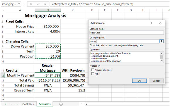
FIGURE 2-9: Creating a scenario for a mortgage analysis.

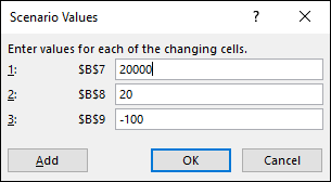
FIGURE 2-10: Example values for a scenario’s changing cells.

Apply a scenario

The real value of a scenario is that no matter how many changing cells you’ve defined or how complicated the formula is, you can apply any scenario with just a few straightforward steps. Don’t believe me? Here, I’ll prove it:

1. Choose Data ⇒ What-If Analysis ⇒ Scenario Manager.

   The Scenario Manager dialog box appears.

2. Select the scenario you want to display.

3. Click Show.

   Without even a moment’s hesitation, Excel enters the scenario values into the changing cells and displays the formula result.

4. Feel free to repeat Steps 2 and 3 to display other scenarios. When it’s this easy, why not?
5. When you’ve completed your analysis, click Close.

Edit a scenario

If you need to make changes to a scenario, you can edit the name, the changing cells, the description, and the scenario’s input values. Here are the steps to follow:

1. Choose Data ⇒ What-If Analysis ⇒ Scenario Manager.

   The Scenario Manager dialog box appears.

2. Select the scenario you want to modify.

3. Click Edit.

   The Edit Scenario dialog box appears.

4. Modify the scenario name, changing cells, and comment, as needed.

5. Click OK.

   The Scenario Values dialog box appears.

6. Modify the scenario values, as needed.
7. Click OK.
8. Click Close.

Delete a scenario

If you have a scenario that has worn out its welcome, you should delete it to reduce clutter in the Scenario Manager. Here are the steps required:

1. Choose Data ⇒ What-If Analysis ⇒ Scenario Manager.

   The Scenario Manager dialog box appears.

2. Select the scenario you want to remove.

   Excel does not ask you to confirm the deletion, so double- (perhaps even triple-) check that you’ve selected the correct scenario.

3. Click Delete.

   The Scenario Manager gets rids of the scenario.

4. Click Close.

Optimizing Data with Solver

Spreadsheet tools such as Goal Seek that change a single variable are useful, but unfortunately most problems in business are not so easy. You’ll usually face formulas with at least two and sometimes dozens of variables. Often, a problem will have more than one solution, and your challenge will be to find the optimal solution (that is, the one that maximizes profit, or minimizes costs, or matches other criteria). For these bigger challenges, you need a more muscular tool. Excel has just the answer: Solver. Solver is a sophisticated optimization program that enables you to find the solutions to complex problems that would otherwise require high-level mathematical analysis.

Understanding Solver

Solver, like Goal Seek, uses an iterative method to perform its calculations. Using iteration means that Solver tries a solution, analyzes the results, tries another solution, and so on. However, this cyclic iteration isn’t just guesswork on Solver’s part. That would be silly. No, Solver examines how the results change with each new iteration and, through some sophisticated mathematical processes (which, thankfully, happen way in the background and can be ignored), can usually tell in what direction it should head for the solution.

The advantages of Solver

Yes, Goal Seek and Solver are both iterative, but that doesn’t make them equal. In fact, Solver brings a number of advantages to the table:

• Solver enables you to specify multiple adjustable cells. You can use up to 200 adjustable cells in all.
• Solver enables you to set up constraints on the adjustable cells. For example, you can tell Solver to find a solution that not only maximizes profit, but also satisfies certain conditions, such as achieving a gross margin between 20 and 30 percent, or keeping expenses less than $100,000. These conditions are said to be constraints on the solution.
• Solver seeks not only a desired result (the “goal” in Goal Seek) but also the optimal one. For example, looking for an optimal result might mean that you can find a solution that’s the maximum or minimum possible.
• For complex problems, Solver can generate multiple solutions. You can then save these different solutions under different scenarios.

When should you use Solver?

Okay, I’ll be straight with you: Solver is a powerful tool that most Excel users don’t need. It would be overkill, for example, to use Solver to compute net profit given fixed revenue and cost figures. Many problems, however, require nothing less than the Solver approach. These problems cover many different fields and situations, but they all have the following characteristics in common:

• They have a single objective cell (also called the target cell) that contains a formula you want to maximize, minimize, or set to a specific value. This formula could be a calculation such as total transportation expenses or net profit.
• The objective cell formula contains references to one or more variable cells (also called unknowns or changing cells). Solver adjusts these cells to find the optimal solution for the objective cell formula. These variable cells might include items such as units sold, shipping costs, or advertising expenses.
• Optionally, there are one or more constraint cells that must satisfy certain criteria. For example, you might require that advertising be less than 10 percent of total expenses, or that the discount to customers be an amount between 40 and 60 percent.

For example, Figure 2-11 shows a worksheet data model that’s all set up for Solver. The model shows revenue (price times units sold) and costs for two products, the profit produced by each products, and the total profit. The question to be answered here is this: How many units of each product must be sold to get a total profit of $0? This is known in business as a break-even analysis.

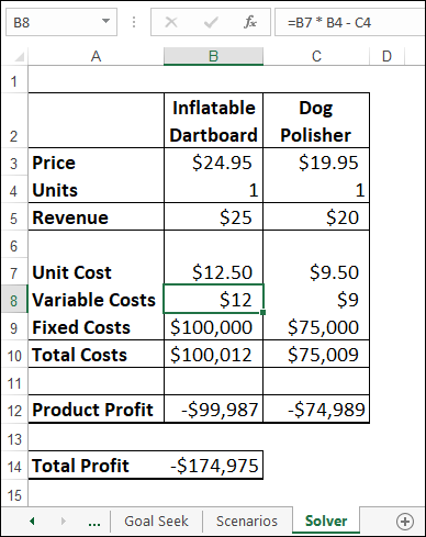
FIGURE 2-11: The goal for this data model is to find the break-even point (where total profit is $0).

That sounds like a straightforward Goal Seek task, but this model has a tricky aspect: the variable costs. Normally, the variable costs of a product are its unit cost times the number of units sold. If it costs $10 to produce product A, and you sell 10,000 units, the variable costs for that product are $100,000. However, in the real world, such costs are often mixed up among multiple products. For example, if you run a joint advertising campaign for two products, those costs are borne by both products. Therefore, this model assumes that the costs of one product are related to the units sold of the other. Here, for example, is the formula used to calculate the costs of the Inflatable Dartboard (cell B8):

=B7 * B4 – C4

In other words, the variable costs for the Inflatable Dartboard are reduced by one dollar for every unit sold of the Dog Polisher. The latter’s variable costs use a similar formula (in cell C8):

=C7 * C4 – B4

Having the variable costs related to multiple products puts this data model outside of what Goal Seek can do, but Solver is up to the challenge. Here are the special cells in the model that Solver will use:

• The objective cell is C14; the total profit and the target solution for this formula is 0 (that is, the break-even point).
• The changing cells are B4 and C4, which hold the number of units sold for each product.
• For constraints, you might want to add that both the product profit cells (B12 and C12) should also be 0.

Loading the Solver add-in

An add-in is software that adds one or more features to Excel. Installing add-ins gives you additional Excel features that aren’t available in the Ribbon by default. Bundled add-in software is included with Excel but isn’t automatically installed when you install Excel. Several add-ins come standard with Excel, including Solver, which enables you to solve optimization problems.

You install the bundled add-ins by using the Excel Options dialog box; you can find them in the Add-Ins section. After they're installed, add-ins are available right away. They usually appear on a tab related to their function. For example, Solver appears on the Data tab.

Here are the steps to follow to load the Solver add-in:

1. Choose File ⇒ Options.

   The Excel Options dialog box appears.

2. Choose Add-Ins.

3. In the Manage list, select Excel Add-Ins and then select Go.

   Excel displays the Add-Ins dialog box.

4. Select the Solver Add-In check box

5. Click OK.

   Excel adds a Solver button to the Data tab’s Analyze group.

Optimizing a result with Solver

You set up your Solver model by using the Solver Parameters dialog box. You use the Set Objective box to specify the objective cell, and you use the To group to tell Solver what you want from the objective cell: the maximum possible value; the minimum possible value; or a specific value. Finally, you use the By Changing Variable Cells box to specify the cells that Solver can use to plug in values to optimize the result.

When Solver finds a solution, you can choose either Keep Solver Solution or Restore Original Values. If you choose Keep Solver Solution, Excel permanently changes the worksheet. You cannot undo the changes.

With your Solver-ready worksheet model ready to go, here are the steps to follow to find an optimal result for your model using Solver:

1. Choose Data ⇒ Solver.

   Excel opens the Solver Parameters dialog box.

2. In the Set Objective box, enter the address of your model’s objective cell.

   In the example in the “When should you use Solver?” section, earlier in the chapter (refer to Figure 2-11), the objective cell is B14. Note that if you click the cell to enter it, Solver automatically enters an absolute cell address (for example, $B$14 instead of B14). Solver works fine either way.

3. In the To group, select an option:

   • Max: Returns the maximum possible value.
   • Min: Returns the minimum possible value.
   • Value Of: Enter a number to set the objective cell to that number.

   For the example model, I select Value Of and enter 0 in the text box.

4. In the By Changing Variable Cells box, enter the addresses of the cells you want Solver to change while it looks for a solution.

   In the example, the changing cells are B4 and C4. Figure 2-12 shows the completed Solver Parameters dialog box. (What about constraints? I talk about those in the next section.)

5. Click Solve.

   Solver gets down to business. As Solver works on the problem, you might see the Show Trial Solution dialog boxes show up one or more times.

6. In any Show Trial Solution dialog box that appears, click Continue to move things along.

   When the optimization is complete, Excel displays the Solver Results dialog box, shown in Figure 2-13.

7. Select the Keep Solver Solution option.

   If you don't want to accept the result, select the Restore Original Values option instead.

8. Click OK.

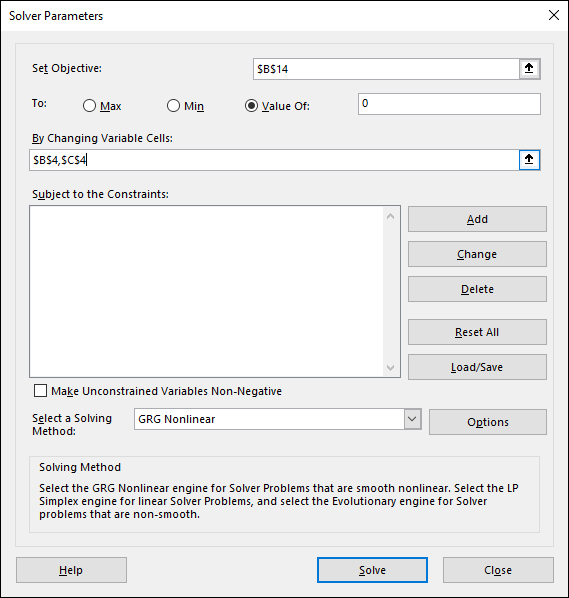
FIGURE 2-12: The completed Solver Parameters dialog box.

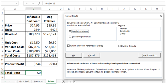
FIGURE 2-13: The Solver Results dialog box and the solution to the break-even problem.

You can ask Solver to display one or more reports that give you extra information about the results. In the Solver Results dialog box, use the Reports list to select each report you want to view:

• Answer: Displays information about the model’s objective cell, variable cells, and constraints. For the objective cell and variable cells, Solver shows the original and final values.
• Sensitivity: Attempts to show how sensitive a solution is to changes in the model’s formulas. The layout of the Sensitivity report depends on the type of model you’re using.
• Limits: Displays the objective cell and its value, as well as the variable cells and their addresses, names, and values.

Solver can use one of several solving methods. In the Solver Parameters dialog box, use the Select a Solving Method list to select one of the following:

• Simplex LP: Use if your worksheet model is linear. In the simplest possible terms, a linear model is one in which the variables are not raised to any powers and none of the so-called transcendent functions — such as SIN and COS — are used.
• GRG Nonlinear: Use if your worksheet model is nonlinear and smooth. In general terms, a smooth model is one in which a graph of the equation used doesn’t show sharp edges or breaks.
• Evolutionary: Use if your worksheet model is nonlinear and nonsmooth.

Do you have to worry about any of this? Almost certainly not. Solver defaults to using GRG Nonlinear, and that should work for almost anything you do with Solver.

Adding constraints to Solver

The real world puts restrictions and conditions on formulas. A factory might have a maximum capacity of 10,000 units a day, the number of employees in a company can’t be a negative number, and your advertising costs might be restricted to 10 percent of total expenses.

Similarly, suppose that you’re running a break-even analysis on two products, as I discuss in the previous section. If you run the optimization without any restrictions, Solver might reach a total profit of 0 by setting one product at a slight loss and the other at a slight profit, where the loss and profit cancel each other out. In fact, if you take a close look at Figure 2-13, this is exactly what Solver did. To get a true break-even solution, you might prefer to see both product profit values as 0.

Such restrictions and conditions are examples of what Solver calls constraints. Adding constraints tells Solver to find a solution so that these conditions are not violated.

Here’s how to run Solver with constraints added to the optimization:

1. Choose Data ⇒ Solver.

   Excel opens the Solver Parameters dialog box.

2. Use the Set Objective box, the To group, and the By Changing Variable Cells box to set up Solver as I describe in the previous section, “Optimizing a result with Solver.”

3. Click Add.

   Excel displays the Add Constraint dialog box.

4. In the Cell Reference box, enter the address of the cell you want to constrain.

   You can type the address or select the cell on the worksheet.

5. In the drop-down list, select the operator you want to use.

   Most of the time, you use a comparison operator, such as equal to (=) or greater than (>). Use the int (integer) operator when you need a constraint, such as total employees, to be an integer value instead of a real number (that is, a number with a decimal component; you can't have 10.5 employees!). Use the bin (binary) operator when you have a constraint that must be either TRUE or FALSE (or 1 or 0).

6. If you chose a comparison operator in Step 5, in the Constraint box, enter the value by which you want to restrict the cell.

   Figure 2-14 shows an example of a completed Add Constraint dialog box. In the example model, this constraint tells Solver to find a solution such that the product profit of the Inflatable Dartboard (cell B12) is equal to 0.

7. To specify more constraints, click Add and repeat Steps 4 through 6, as needed.

   For the example, you add a constraint that asks for the Dog Polisher product profit (cell C12) to be 0.

8. Click OK.

   Excel returns to the Solver Parameters dialog box and displays your constraints in the Subject to the Constraints list box.

9. Click Solve.

10. In any Show Trial Solution dialog box that appears, click Continue to move things along.

    Figure 2-15 shows the example break-even solution with the constraints added. Notice that not only is the Total Profit cell (B14) set to 0, but so are the two Product Profit cells (B12 And C12).

11. Select the Keep Solver Solution option.

    If you don’t want to accept the result, select the Restore Original Values option instead.

12. Click OK.

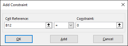
FIGURE 2-14: The completed Add Constraint dialog box.

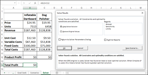
FIGURE 2-15: The Solver Results dialog box and the final solution to the break-even problem.

You can add a maximum of 100 constraints. Also, if you need to make a change to a constraint before you begin solving, select the constraint in the Subject to the Constraints list box, click Change, and then make your adjustments in the Change Constraint dialog box that appears. If you want to delete a constraint that you no longer need, select the constraint and then click Delete.

Save a Solver solution as a scenario

Whenever you have a spreadsheet model that uses a coherent set of input values — known as changing cells — you have what Excel calls a scenario. With Solver, these changing cells are its variable cells, so a Solver solution amounts to a kind of scenario. However, Solver does not give you an easy way to save and rerun a particular solution. To work around this problem, you can save a solution as a scenario that you can then later recall using Excel’s Scenario Manager feature.

Follow these steps to save a Solver solution as a scenario:

1. Choose Data ⇒ Solver.

   Excel opens the Solver Parameters dialog box.

2. Use the Set Objective box, the To group, the By Changing Variable Cells box, and the Subject to the Constraints list to set up Solver as I describe in the “Optimizing a result with Solver” section, earlier in this chapter.
3. Click Solve.

4. Anytime the Show Trial Solution dialog box appears, choose Continue.

   When the optimization is complete, Excel displays the Solver Results dialog box.

5. Click Save Scenario.

   Excel displays the Save Scenario dialog box.

6. In the Scenario Name dialog box, type a name for the scenario and then click OK.

   Excel returns you to the Solver Results dialog box.

7. Select the Keep Solver Solution option.

   If you don’t want to accept the result, select the Restore Original Values option instead.

8. Click OK.