Chapter 8

Performing PivotTable Calculations

IN THIS CHAPTER

Trying some PivotTable summary calculations

Working with PivotTable subtotals

Using custom PivotTable calculations

Creating a custom calculated PivotTable field and item

The near-ridiculous power and flexibility of a PivotTable is in contrast with the relative simplicity of what a PivotTable actually does, which is to take a mountain of data and turn it into a molehill of a report. With that report in place, the fun part begins when you pivot fields, group items, and filter the report (all of which I describe in painstaking detail in Chapter 7). Pivoting, grouping, and filtering represent the most visible aspects of a PivotTable’s power, but lots of impressive things happening behind the PivotTable scenes as well. These “hidden” features include the massive number of calculations that Excel performs to summarize all that data so succinctly. That display of raw calculation horsepower is impressive enough, but you can actually harness that power for your own ends.

In this chapter, you open the PivotTable’s hood to check out its calculation engine. You explore how the calculations work, swap out some parts to try different calculations, and even learn how to soup things up with your own custom calculations. Vroom vroom!

Messing around with PivotTable Summary Calculations

The calculation that Excel uses to populate the PivotTable data area is called the summary calculation. Most of the time, the default Sum calculation will get the job done, but Excel offers lots of options for taking the summary calculation to a higher analytical level. The next few sections fill you in on those options.

Changing the PivotTable summary calculation

The default summary calculation depends on the type of field you add to the data area:

• If you add a numeric field to the data area, Excel uses Sum as the default summary calculation.
• If you use a text field in the data area, Excel uses Count as the default summary calculation.

Sum and Count aren’t the only calculation choices, however. If your data analysis requires a different calculation, you can configure the data field to use any one of Excel’s 11 built-in summary calculations. Here’s the complete list:

• Average: Calculates the mean value in a numeric field.
• Count: Displays the total number of cells in the source field.
• Count Numbers: Displays the total number of numeric values in the source field.
• Max: Displays the largest value in a numeric field.
• Min: Displays the smallest value in a numeric field.
• Product: Multiplies the values in a numeric field.
• StdDev: Calculates the standard deviation of a population sample, which tells you how much the values in the source field vary with respect to the average.
• StdDevp: Calculates the standard deviation when the values in the data field represent the entire population.
• Sum: Adds the values in a numeric field.
• Var: Calculates the variance of a population sample, which is the square of the standard deviation.
• Varp: Calculates the variance when the values in the data field represent the entire population.

Here are the steps to follow to try a different summary calculation:

1. Select any cell in the data field.

2. Choose Analyze ⇒ Field Settings.

   The Value Field Settings dialog box appears with the Summarize Values By tab displayed, as shown in Figure 8-1.

3. In the Summarize Value Field By list, select the summary calculation you want to use.

4. Click OK.

   Excel recalculates the PivotTable results and renames the value field label to reflect the new summary calculation.

FIGURE 8-1: Use the Value Field Settings dialog box to choose a summary calculation.

Another way to change the PivotTable summary calculation is to right-click any cell in the value field, choose the Summarize Values By command, and then select the calculation you want to use from the submenu that appears. If you don’t see the calculation, choose the More Options command to open the Value Field Settings dialog box.

When you build your PivotTable, you may find that the results don’t pass the smell test. For example, the numbers may appear to be far too small. In that case, check the summary calculation that Excel has applied to the field to see whether it’s using Count instead of Sum. If the data field includes one or more text cells or one or more blank cells, Excel defaults to the Count summary function instead of Sum. If your field is supposed to be numeric, check the data to see whether any text values or blank cells are showing up.

When you add a second field to the row or column area, Excel displays a subtotal for each item in the outer field. (The outer field is the field “farthest” from the value area: the leftmost field if you have two fields in the row area; the topmost field if you have two fields in the column area. The other field is called the inner field because it’s “closest” to the value area.) By default, the subtotals show the sum of the data results for each outer field item. However, the same 11 summary calculations — from Average to Varp — are also available for subtotals.

Trying out the difference summary calculation

The built-in summary calculations — Sum, Count, and so on — apply over an entire field. However, a major part of data analysis involves comparing one item with another. If you’re analyzing sales to customers, for example, knowing how much you sold this year is useful, but even more useful is to compare this year’s sales with last year’s. Are the sales up or down? By how much? Are the sales up or down with all customers or only some? These are fundamental questions that help managers run departments, divisions, and companies.

Excel offers two difference calculations that can help with this kind of analysis:

• Difference From: Compares one numeric item with another and returns the difference between them
• % Difference From: Compares one numeric item with another and returns the percentage difference between them

Before you set up a difference calculation, you need to decide which field in your PivotTable to use as the comparison field, or base field, and which item within that field to use as the basis for all the comparisons, which is called the base item. For example, take a peek at Figure 8-2, which uses the Order Date field to show the sales in 2019 and the sales in 2018. In this example, Order Date is the base field and 2018 is the base item.

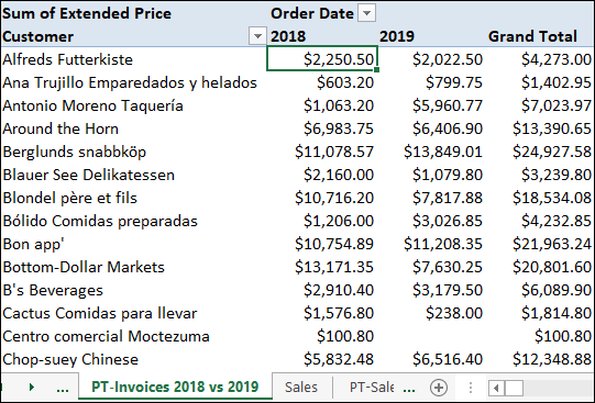
FIGURE 8-2: A PivotTable that shows sales in two years: 2018 and 2019.

Here are the steps to follow to apply a difference summary calculation to a PivotTable:

1. Select any cell in the value field.

2. Choose Analyze ⇒ Field Settings.

   The Value Field Settings dialog box appears with the Summarize Values By tab displayed.

3. Click the Show Values As tab.

4. In the Show Values As list, select Difference From.

   If you want to see the difference in percentage terms, select % Difference From instead.

   Another way to select the Difference Summary calculation is to right-click any cell in the value field, select Show Values As, and then select Difference From.

5. In the Base Field list, select the field from which you want Excel to calculate the difference.

6. In the Base Item list, select a base item.

   Figure 8-3 shows a completed Show Values As tab for the example PivotTable.

7. Click OK.

   Excel recalculates the PivotTable results to show the difference summary calculation. Figure 8-4 shows the PivotTable from Figure 8-2 with the Difference From calculation applied.

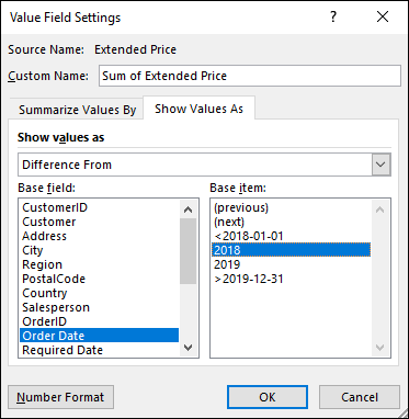
FIGURE 8-3: Use the Value Field Settings dialog box to choose a summary calculation.

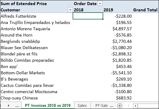
FIGURE 8-4: The PivotTable from Figure 8-2 is now using the Difference From calculation.

Applying a percentage summary calculation

When analyzing data, comparing two or more items as a percentage is often helpful because percentage calculations enable you to make apples-to-apples comparisons between values. For example, if your PivotTable shows quarterly sales by region (see Figure 8-5), you might want to know how the results in the second, third, and fourth quarters compare, as a percentage, to the results from the first quarter.

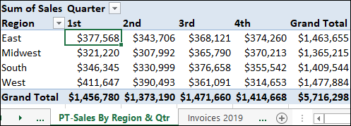
FIGURE 8-5: A PivotTable that shows quarterly sales by region.

That kind of comparison sounds hard, but you can use Excel’s percentage calculations to quickly view data items as a percentage of some other item or as a percentage of the total in the current row, column, or PivotTable. Excel offers seven percentage calculations that can help you perform this kind of analysis:

• % Of: Returns the percentage of each value with respect to a selected base item.
• % of Row Total: Returns the percentage that each value in a row represents of the total value of the row.
• % of Column Total: Returns the percentage that each value in a column represents of the total value of the column.
• % of Grand Total: Returns the percentage that each value represents of the PivotTable grand total.
• % of Parent Row Total: If you have multiple fields in the row area, this calculation returns the percentage that each value in an inner row represents with respect to the total of the parent item in the outer row.
• % of Parent Column Total: If you have multiple fields in the column area, this calculation returns the percentage that each value in an inner column represents with respect to the total of the parent item in the outer column.
• % of Parent Total: If you have multiple fields in the row or column area, this calculation returns the percentage of each value with respect to a selected base field in the outer row or column.

If you use the % Of or the % of Parent Total calculation, you must also choose a base field and a base item upon which Excel will calculate the percentages.

Here are the steps to follow to apply a percentage summary calculation:

1. Select any cell in the value field.

2. Choose Analyze ⇒ Field Settings.

   The Value Field Settings dialog box appears with the Summarize Values By tab displayed.

3. Click the Show Values As tab.

4. In the Show Values As list, select the percentage calculation you want to use.

   If you select % Of or % of Parent Total, continue with Step 5; otherwise, skip to Step 7.

5. In the Base Field list, select the field from which you want Excel to calculate the percentages.
6. In the Base Item list, select a base item.

7. Click OK.

   Excel recalculates the PivotTable results to show the percentage summary calculation. Figure 8-6 shows the PivotTable from Figure 8-2 with the % Of calculation applied.

FIGURE 8-6: The PivotTable from Figure 8-5, now using the % Of calculation.

Adding a running total summary calculation

A running total is the cumulative sum of the values that appear in a given set of data. Most running totals accumulate over a period of time. For example, suppose you have 12 months of sales figures. In a running total calculation, the first value is the first month of sales, the second value is the sum of the first and second months, the third value is the sum of the first three months, and so on.

You use a running total in data analysis when you need to see a snapshot of the overall data at various points. For example, suppose you have a sales budget for each month. As the fiscal year progresses, comparing the running total of the budget figures with the running total of the actual sales tells you how your department or company is doing with respect to the budget. If sales are consistently below budget, you might consider lowering prices, offering customers extra discounts, or increasing your product advertising.

Creating a running total seems like a job best left to a complex Excel formula. Sure, you could create such a formula, but I’m happy to report that you don’t have to bother with any of that. That’s because Excel offers a built-in Running Total In summary calculation that you can apply to your PivotTable results. No muss and not even any fuss.

The Running Total In summary applies to not just the Sum calculation but also related calculations, such as Count and Average.

Before you configure your PivotTable to use a Running Total In summary calculation, you must choose the field on which to base the accumulation, called the base field. This field will most often be a date field, but you can also create running totals based on other fields, such as customer, division, product, and so on.

Here are the steps to follow to apply a Running Total In summary calculation to a PivotTable:

1. Select any cell in the value field.

2. Choose Analyze ⇒ Field Settings.

   The Value Field Settings dialog box appears with the Summarize Values By tab displayed.

3. Click the Show Values As tab.

4. In the Show Values As list, select Running Total In.

   If you want to see the running total in percentage terms, select % Running Total In instead.

   Another way to select the Running Total In summary calculation is to right-click any cell in the value field, and then choose Show Values As  ⇒ Running Total In.

5. In the Base Field list, select the field from which you want Excel to accumulate the running totals.

6. Click OK.

   Excel recalculates the PivotTable results to show the running totals. Figure 8-8 shows the PivotTable from Figure 8-7 with the Running Total In calculation applied.

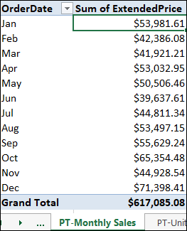
FIGURE 8-7: A PivotTable showing monthly order totals.

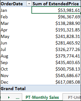
FIGURE 8-8: The PivotTable from Figure 8-7, with the Running Total In calculation applied.

Creating an index summary calculation

One of the most crucial aspects of data analysis is determining the relative importance of the results of your calculations. This determination is particularly vital in a PivotTable, whose results summarize a large amount of data but on the surface provide no clue as to the relative importance of the various value area results.

For example, suppose your PivotTable shows the units sold for various product categories broken down by region (see Figure 8-9). Suppose further that in Oregon, you sold 30 units of produce and 35 units of seafood. Does this mean that seafood sales are relatively more important in the Oregon market than produce sales? Not necessarily. To determine relative importance, you must take into account the larger picture, such as the total units sold of both produce and seafood across all states. Suppose the produce total is 145 units and the seafood total is 757 units. In that case, you can see that the 30 units of produce sold in Oregon represents a much higher portion of total produce sales than does Oregon’s 35 units of seafood. A proper analysis would also take into account the total units sold in Oregon and the total units sold overall (the PivotTable’s Grand Total).

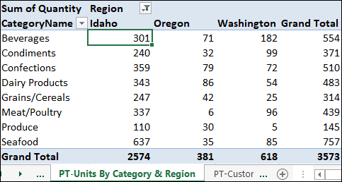
FIGURE 8-9: A PivotTable showing units sold by category and region.

Determining the relative importance of a PivotTable’s results sounds headache-inducingly complex, but Excel offers the built-in Index calculation, which handles everything without the need for aspirin. The Index calculation determines the weighted average — the average taking into account the relative importance of each value — of each cell in the PivotTable results.

Put your math geek hat on because here’s the formula Excel uses:

(Cell Value) * (Grand Total) / (Row Total) * (Column Total)

In the Index calculation results, the higher the value, the more important the cell is in the overall PivotTable report.

Follow these steps to apply the Index summary calculation to a PivotTable:

1. Select any cell in the value field.

2. Choose Analyze ⇒ Field Settings.

   The Value Field Settings dialog box appears with the Summarize Values By tab displayed.

3. Click the Show Values As tab.

4. In the Show Values As list, select Index.

   Alternatively, right-click any cell in the value field, and then choose Show Values As ⇒ Index.

5. Click OK.

   Excel recalculates the PivotTable results to show the Index results.

Working with the Index calculation results is much easier if you format the data field to show just two decimal places. Select any cell in the value field, choose Analyze ⇒ Field Settings, click Number Format, select Number in the Category list, make sure that 2 appears in the Decimal places field, click OK, and then click OK again.

Figure 8-10 shows the PivotTable from Figure 8-9 with the Index calculation applied. Notice that under Oregon, the index value for the Produce category is 1.94, whereas the index value for Seafood is 0.43, which tells you that produce sales in Oregon are relatively more important than seafood sales.

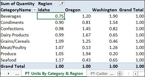
FIGURE 8-10: The PivotTable from Figure 8-9, with the Index calculation applied.

Working with PivotTable Subtotals

When you add a second field to the row or column area, as I describe in Chapter 7, Excel displays subtotals for the items in the outer field. Having these outer field subtotals available is a useful component of data analysis because it shows you not only how the data breaks down according to the items in the second (inner) field, but also the total of those items for each item in the first (outer) field. However, Excel lets you turn off subtotals that you don't want to see, and it lets you add multiple subtotals. The next two sections provide the details.

Turning off subtotals for a field

If you kick things up a notch and add a third field to the row or column area, Excel displays two sets of subtotals: one for the second (middle) field and one for the first (outer) field. And for every extra field you add to the row or column area, Excel mindlessly adds yet another set of subtotals.

Believe me, a PivotTable displaying two or more sets of subtotals in one area is no picnic to read. Do yourself a favor and reduce the complexity of the PivotTable layout by turning off the subtotals for one or more of the fields. Here’s how:

1. Select any cell in the field you want to work with.

2. Choose Analyze ⇒ Field Settings.

   The Field Settings dialog box appears with the Subtotals & Filters tab displayed.

3. In the Subtotals group, select the None radio button.

   Alternatively, right-click any cell in the field and then deselect the Subtotal “Field” command, where Field is the name of the field.

4. Click OK.

   Excel hides the field’s subtotals.

Displaying multiple subtotals for a field

When you add a second field to the row or column area, as I discuss in Chapter 7, Excel displays a subtotal for each item in the outer field, and that subtotal uses the Sum calculation. If you prefer to see the Average for each item or the Count, you can change the field’s summary calculation; see the section “Changing the PivotTable summary calculation,” earlier in this chapter.

However, a common data analysis task is to view items from several different points of view. That is, you study the results by eyeballing not just a single summary calculation, but several: Sum, Average, Count, Max, Min, and so on.

That’s awesome of you, but it’s not all that easy to switch from one summary calculation to another. To avoid this problem, Excel enables you to view multiple subtotals for each field, with each subtotal using a different summary calculation. It’s true. You can use as many of Excel’s 11 built-in summary calculations as you need. That said, however, I should point out that using StdDev and StDevp at the same time doesn't make sense, because the former is for sample data and the latter is for population data. The same is true for the Var and Varp calculations.

Okay, here are the steps to follow to add multiple subtotals to a field:

1. Select any cell in the field you want to mess with.

2. Choose Analyze ⇒ Field Settings.

   The Field Settings dialog box appears with the Subtotals & Filters tab displayed.

3. In the Subtotals group, select the Custom radio button.

4. In the list that appears below the Custom options, select each calculation that you want to appear as a subtotal.

   Alternatively, right-click any cell in the field and then deselect the Subtotal “Field” command, where Field is the name of the field.

5. Click OK.

   Excel recalculates the PivotTable to show the subtotals you selected. Figure 8-11 shows an example PivotTable showing the Sum, Average, Max, and Min subtotals.

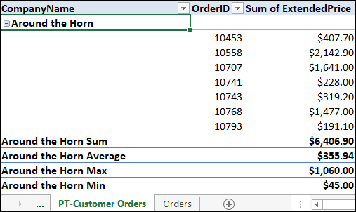
FIGURE 8-11: A PivotTable with multiple subtotals.

Introducing Custom Calculations

A custom calculation is a formula that you define yourself to produce PivotTable values that wouldn’t otherwise appear in the report if you used only the source data and Excel’s prefab summary calculations. Custom calculations let you to extend your data analysis to include results that are tailored to your company, department, or the daily whims of your boss.

For example, suppose your PivotTable shows employee sales by quarter and you want to award a 10 percent bonus to each employee with sales of more than $50,000 in any quarter. That’s awfully generous of you! To help, you can create a custom calculation that checks for sales greater than $50,000 and then multiplies those by 0.1 to get the bonus number.

A custom calculation is an Excel formula that’s applied to your source data to produce a summary result. In other words, in most cases the custom calculation is just like Excel’s built-in PivotTable summary calculations, except that you define the specifics of the calculation yourself. Because you’re creating a formula, you can use most of Excel’s formula power, which gives you tremendous flexibility to create custom calculations that suit your data-analysis needs. And by placing these calculations within the PivotTable itself — as opposed to, for example, adding them to your source data — you can easily update the calculations as needed and refresh the report results.

Formulas for custom calculations

Custom calculations are formulas with certain restrictions imposed; see the section “Understanding custom calculation limitations,” later in this chapter, for more details. A custom calculation formula always begins with an equals sign (=), followed by one or more operands and operators:

• Operands: The values that the formula uses as the raw material for the calculation. In a custom PivotTable calculation, the operands can be numbers, worksheet functions, or fields from your data source.
• Operators: The symbols that the formula uses to perform the calculation. In a custom PivotTable calculation, the available operators include addition (+), subtraction (–), multiplication (*), division (/), and comparison operators such as greater than (>) and less than or equal to (<=).

Checking out the custom calculation types

When building a custom calculation for a PivotTable, Excel offers two types:

• Calculated field: A new data field in which the values are the result of a custom calculation formula. You can display the calculated field along with another data field or on its own. A calculated field is really a custom summary calculation, so in almost all cases, the calculated field references one or more fields in the source data. See the section “Inserting a Custom Calculated Field,” later in this chapter.
• Calculated item: A new item in a row or column field in which the values are the result of a custom calculation. In this case, the calculated item’s formula references one or more items in the same field. See the section “Inserting a Custom Calculated Item,” later in this chapter, for more on working with a custom calculated item.

Understanding custom calculation limitations

Custom calculations — whether they’re calculated fields or calculated items — are powerful additions to your PivotTable analysis toolbox. However, although custom calculation formulas look like regular worksheet formulas, you can’t assume that you can do everything with a custom PivotTable formula that you can do with a worksheet formula. In fact, Excel imposes a number of limitations on custom formulas.

The major limitation inherent in custom calculations is that, with the exception of constant values such as numbers, you can’t reference anything outside the PivotTable’s source data:

• You can’t use a cell reference, range address, or range name as an operand in a custom calculation formula.
• You can’t use any worksheet function that requires a cell reference, range, or defined name. However, you can still use many of Excel’s worksheet functions by substituting either a PivotTable field or a PivotTable item in place of a cell reference or range name. For example, if you want a calculated item that returns the average of items named Jan, Feb, and Mar, you could use the following formula:

  =AVERAGE(Jan, Feb, Mar)

• You can’t use the PivotTable’s subtotals, row totals, column totals, or Grand Total as an operand in a custom calculation formula.

You also need to understand how references to other PivotTable fields work within your calculations and what limitations you face when using field references:

• Field references: When you reference a PivotTable field in your formula, Excel interprets this reference as the sum of that field’s values. For example, the formula =Sales + 1 does not add 1 to each Sales value and return the sum of these results; that is, Excel does not interpret the formula as =Sum of (Sales + 1). Instead, the formula adds 1 to the sum of the Sales values, and Excel interprets the formula as =(Sum of Sales) + 1.
• Field reference problems: The fact that Excel defaults to a Sum calculation when you reference another field in your custom calculation can lead to problems. The trouble is that summing certain types of data doesn't make sense. For example, suppose you have inventory source data with UnitsInStock and UnitPrice fields. You want to calculate the total value of the inventory, so you create a custom field based on the following formula:

  =UnitsInStock * UnitPrice

• Unfortunately, this formula doesn't work because Excel treats the UnitPrice operand as Sum of UnitPrice. “Adding” the prices together doesn't make sense, so your formula produces an incorrect result.

Finally, Excel imposes the following limitations on the use of calculated items:

• A formula for a calculated item can't reference items from any field except the one in which the calculated item resides.
• You can’t insert a calculated item into a PivotTable that has at least one grouped field. You must ungroup all the PivotTable fields before you can insert a calculated item.
• You can’t group a field in a PivotTable that has at least one calculated item.
• You can’t insert a calculated item into a filter field. Also, you can’t move a row or column field that has a calculated item into the filter area.
• You can’t insert a calculated item into a PivotTable in which a field has been used more than once.
• You can’t insert a calculated item into a PivotTable that uses the Average, StdDev, StdDevp, Var, or Varp summary calculations.

Inserting a Custom Calculated Field

A custom calculated field might look much like an Excel worksheet formula, but you don’t enter the formula for a calculated field into a worksheet cell. Instead, Excel offers the Calculated Field feature, which provides a dialog box for you to name the field and construct the formula. Excel then stores the formula along with the rest of the PivotTable data.

Here are the steps to follow to insert a custom calculated field into a PivotTable:

1. Select any cell inside the PivotTable’s value area.

2. Choose Analyze ⇒ Fields, Items, & Sets ⇒ Calculated Field.

   The Insert Calculated Field dialog box appears.

3. In the Name text box, enter a name for the calculated field.

4. In the Formula text box, start the formula.

   Begin with an equals sign (=) and then add any constants or worksheet functions you need to get started.

5. When you get to the point in your formula at which you need to add a field, select a field in the Fields list and then click Insert Field.

   You can also double-click the field to add it to the formula.

6. Keep building your formula, repeating Step 5 to add fields as needed.

7. When the formula is complete, click Add.

   Figure 8-12 shows an example formula for a custom calculated field. In this case, the formula uses an IF() function to check whether the ExtendedPrice field is greater than 50,000. If it is, the formula returns the ExtendedPrice value multiplied by 0.1; otherwise, it returns 0.

8. Click OK.

   Excel adds the calculated field to the PivotTable’s data area, as shown in Figure 8-13. Excel adds the calculated field to the PivotTable Fields pane.

FIGURE 8-12: A custom calculated field, ready for insertion into the PivotTable.

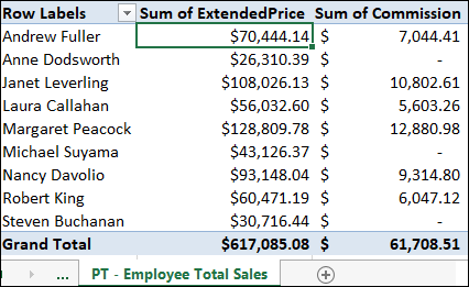
FIGURE 8-13: The custom calculated field in action.

When you add a calculated field to the PivotTable, Excel also applies the custom calculation to the Grand Total value (refer to Figure 8-13). Unfortunately, this total is often inaccurate, and you should be careful not to assume that it’s correct. The problem is that it’s not a sum of the values in the calculated field, as you might think. Instead, Excel applies the calculated field’s formula to the sum of whatever field or fields you referenced in the formula. In the example shown in Figure 8-13, Excel applies the formula to the Sum of Extended Price field’s Grand Total value, which is not the correct way to calculate the total commission. If you want to see the correct total for the calculated field, set up a formula outside the PivotTable that sums the values.

Inserting a Custom Calculated Item

If your data analysis requires PivotTable results that are not available using just the data source fields and Excel’s built-in summary calculations, no problem: You can insert a calculated item that uses a custom formula to derive the results you need. Sweet!

A calculated item uses a formula that's similar to an Excel worksheet formula, but you don’t enter the formula for a calculated item into a worksheet cell. Instead, Excel offers the Calculated Item command, which displays a dialog box in which you name the item and construct the formula. Excel then stores the formula along with the rest of the PivotTable data.

The Calculated Item feature creates just a single item in a field. However, feel free to add as many calculated items as you need. For example, suppose you want to compare the sales of nonvegan items (such as meat, poultry, dairy, and seafood) with vegan items (grains, cereals, produce, and beverages). One approach would be to create one calculated item that returns the average sales of the nonvegan items and a second calculated item that returns the average sales of the vegan items.

Here are the steps to follow to insert a custom calculated item into a PivotTable:

1. Select any cell inside the field to which you want to insert the item.

2. Choose Analyze ⇒ Fields, Items, & Sets ⇒ Calculated Item.

   The Insert Calculated Item dialog box appears.

3. In the Name text box, enter a name for the calculated field.

4. In the Formula text box, start the formula.

   Begin with an equals sign (=) and then add any constants or worksheet functions you need to get started.

5. When you get to the point in your formula at which you need to add a field, select the field in the Fields list and then click Insert Field.

   You can also double-click the field to add it to the formula.

6. When you get to the point in your formula at which you need to add an item, select the item in the Items list and then click Insert Item.

   You can also double-click the item to add it to the formula.

7. Keep building your formula, repeating Steps 5 and 6 to add fields and items as needed.

8. When the formula is complete, click Add.

   Figure 8-14 shows an example formula for a custom calculated item. In this case, I use the AVERAGE() function to calculate the average of several nonvegan food categories.

9. Click OK.

10. Click OK.

    Excel adds the calculated item to the PivotTable field. Figure 8-15 shows two calculated items added to the PivotTable’s row field. Notice, as well, that when you select a custom calculated item, Excel shows the item’s custom formula in the Formula bar.

FIGURE 8-14: A custom calculated item, ready for action.

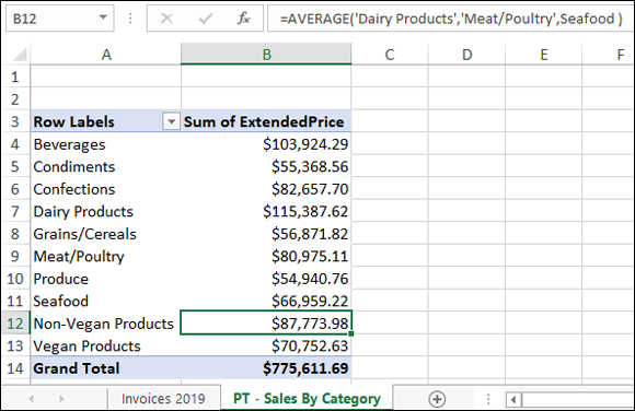
FIGURE 8-15: Two custom calculated items added to the row area.

Editing a Custom Calculation

When you add a custom calculation to a PivotTable, Excel first checks the formula to make sure that it contains no syntax errors — such as a missing comma or parenthesis — or illegal operands — such as cell addresses, unknown field or item names, or functions not supported by custom calculations. If Excel finds an error, it displays a dialog box to scold you and refuses to add the custom calculation to the PivotTable.

However, just because a formula contains no syntax errors or illegal operands doesn’t necessarily mean that its results are correct. In a calculated field, you might have used the wrong function for the result you’re seeking. In a calculated item involving several field items, you might have accidentally missed an item.

Alternatively, your formula may be working perfectly, but it may no longer be the result you need if your data analysis needs have changed. For example, you might have a calculated field that determines whether employees get paid a bonus by looking for sales greater than $50,000. If that threshold changes to $75,000, your calculated field will no longer produce the results you want.

Whether your custom calculation contains an error or your data analysis needs have changed, Excel enables you to edit the formula to produce the result you want. Here’s how to edit a custom calculation:

1. To edit a calculated field, select any cell inside the PivotTable’s data area.

   To edit a calculated item, select any cell inside the field that contains the calculated item.

2. Choose Analyze ⇒ Fields, Items, & Sets  ⇒ Calculated Field.

   The Insert Calculated Field dialog box appears.

   To edit a calculated item instead, choose Analyze ⇒ Fields, Items, & Sets ⇒ Calculated Item to open the Insert Calculated Item dialog box.

3. In the Name list, select the calculation that you want to delete.
4. Edit the formula.
5. Click Modify.

6. Click OK.

   Excel updates the custom calculation’s results.

   You can also edit a calculated item by selecting the item’s result. The formula appears in Excel’s Formula bar, and you can edit it from there.

Deleting a Custom Calculation

Custom calculations don’t always remain a permanent part of a PivotTable report. For example, it’s common to add a calculated field or item temporarily to the PivotTable to test the data or get a number to use elsewhere. Similarly, you may find that you create several versions of a custom calculation and want to keep only the final version. Finally, although custom calculations are a powerful tool, they can’t do everything, so you may find that a calculation does not provide the answer you seek or help you with your data analysis.

For all these situations, Excel enables you to delete those calculated fields or items that you no longer need by following these steps:

1. Select any cell in the PivotTable.

2. To delete a calculated field, choose Analyze ⇒ Fields, Items, & Sets ⇒ Calculated Field.

   The Insert Calculated Field dialog box appears.

   To delete a calculated item instead, choose Analyze ⇒ Fields, Items, & Sets ⇒ Calculated Item to open the Insert Calculated Item dialog box.

3. In the Name list, select the calculation that you want to delete.
4. Click Delete.

5. Click OK.

   Excel removes the custom calculation.