Chapter 3: The Interrupted Gene

3.1 Introduction

The simplest form of a gene is a length of DNA that directly corresponds to its polypeptide product. Bacterial genes are almost always of this type, in which a continuous sequence of 3N bases encodes a polypeptide of N amino acids. However, in eukaryotes, ribosomal RNAs (rRNAs), transfer RNAs (tRNAs), and most messenger RNAs (mRNAs) are first synthesized as long precursor transcripts that are subsequently shortened (see the chapter titled RNA Splicing and Processing). Thus, eukaryotic genes are usually much longer than the functional transcripts they produce. It is reasonable to assume that the shortening involved a trimming of additional, perhaps regulatory, sequences at the 5′ and/or 3′ end of transcripts, leaving the rRNA or protein-encoding sequence of the precursor intact.

However, a eukaryotic gene can include additional sequences that lie both within and outside the region that is operational with respect to phenotype. Protein-encoding sequences can be interrupted, as can the 5′ and 3′ sequences (UTRs) that flank the protein-encoding sequences within mRNA. The interrupting sequences are removed from the primary (RNA) transcript (or pre-mRNA) during gene expression, generating an mRNA that includes a continuous base sequence corresponding to the polypeptide product as determined by the genetic code. The sequences of DNA comprising an interrupted protein-encoding gene are divided into the two categories (see FIGURE 3.1):

FIGURE 3.1 Interrupted genes are expressed via a precursor RNA. Introns are removed when the exons are spliced together. The mature mRNA has only the sequences of the exons.

Exons are the sequences retained in the mature RNA product. A mature transcript begins and ends with exons that correspond to the 5′ and 3′ ends of the RNA.
Introns are the intervening sequences that are removed when the primary RNA transcript is processed to give the mature RNA product.

The exon sequences are in the same order in the gene and in the RNA, but an interrupted gene is longer than its mature RNA product because of the presence of the introns.

The processing of interrupted genes requires an additional step that is not necessary in uninterrupted genes. The DNA of an interrupted gene is transcribed to an RNA copy (a transcript) that is exactly complementary to the original DNA sequence. This RNA is only a precursor, though; it cannot yet be used to produce a polypeptide. First, the introns must be removed from the RNA to give an mRNA that consists only of a series of exons. This process is called RNA splicing (see the chapter titled Genes Are DNA and Encode RNAs and Polypeptides) and involves precisely deleting the introns from the primary transcript and then joining the ends of the RNA on either side of each intron to form a covalently intact molecule (see the chapter titled RNA Splicing and Processing).

The original eukaryotic gene comprises the region in the genome between points corresponding to the 5′ and 3′ terminal bases of mature RNA. We know that transcription begins at the DNA template corresponding to the 5′ end of the mRNA and usually extends beyond the complement to the 3′ end of the mature RNA, which is generated by cleavage of the 3′ extension. The gene is also considered to include the regulatory regions on both sides of the gene that are required for the initiation and (sometimes) termination of transcription.

3.2 An Interrupted Gene Has Exons and Introns

How does the existence of introns change our view of the gene? During splicing, the exons are always joined together in the same order they are found in the original DNA, so the correspondence between the gene and polypeptide sequences is maintained. FIGURE 3.2 shows that the order of exons in a gene remains the same as the order of exons in the processed mRNA, but the distances between sites in the gene do not correspond to the distances between sites in the processed mRNA. The length of a gene is defined by the length of the primary mRNA transcript instead of the length of the mature mRNA. All exons of a gene are on one RNA molecule, and their splicing together is an intramolecular reaction. There is usually no joining of exons carried by different RNA molecules, so there is rarely cross-splicing of sequences. (However, in a process known as trans-splicing, sequences from different mRNAs are ligated together into a single molecule for translation.)

FIGURE 3.2 Exons remain in the same order in mRNA as in DNA, but distances along the gene do not correspond to distances along the mRNA or polypeptide products. The distance from A–B in the gene is smaller than the distance from B–C, but the distance from A–B in the mRNA (and polypeptide) is greater than the distance from B–C.

Mutations that directly affect the sequence of a polypeptide must occur in exons. What are the effects of mutations in the introns? The introns are not part of the mature mRNA, so mutations in them cannot directly affect the polypeptide sequence. However, they can affect the processing of the mRNA production by inhibiting the splicing of exons. A mutation of this sort acts only on the allele that carries it.

Mutations that affect splicing are usually deleterious. The majority are single-base substitutions at the junctions between introns and exons. They might cause an exon to be left out of the product, cause an intron to be included, or make splicing occur at a different site. The most common outcome is a termination codon that shortens the polypeptide sequence. Thus, intron mutations can affect not only the production of a polypeptide but also its sequence. About 15% of the point mutations that cause human diseases disrupt splicing.

Some eukaryotic genes are not interrupted and, like prokaryotic genes, correspond directly with the polypeptide product. In the yeast Saccharomyces cerevisiae, most genes are uninterrupted. In multicellular eukaryotes most genes are interrupted, and the introns are usually much longer than exons so that genes are considerably larger than their coding regions.

3.3 Exon and Intron Base Compositions Differ

In the 1940s, Erwin Chargaff initiated studies of DNA base composition that led to four “rules,” beginning with the first parity rule for duplex DNA (see the chapter titled Genes Are DNA and Encode RNAs and Polypeptides). This rule applies to most regions of DNA, including both exons and introns. Base A in one strand of the duplex is matched by a complementary base (T) in the other strand, and base G in one strand of the duplex is matched by a complementary base (C) in the other strand. By extension, the rule applies not only to single bases but also to dinucleotides, trinucleotides, and oligonucleotides. Thus, GT pairs with its reverse complement AC, and ATG pairs with its reverse complement CAT. In addition to the well-known first parity rule, later work by Chargaff led him to propose a second parity rule. The little-known second parity rule is that, to a close approximation, there are equal amounts of A and T, and equal amounts of C and G, in each single strand of the duplex. Like the first parity rule, this extends to oligonucleotide sequences: For example, in a very long strand there are approximately equal numbers of AC and TG dinucleotides. The reasons for the existence of this rule are not clear, but sequencing of many genomes has shown it to be nearly universally true. The second parity rule applies more closely to introns than to exons, partly due to a further rule—purines tend to cluster on one DNA strand and pyrimidines tend to cluster on the other. This cluster rule as applied to exons is that the purines, A and G, tended to be clustered in one DNA strand of the DNA duplex (usually the nontemplate strand) and these are complemented by clusters of the pyrimidines, T and C, in the template strand.

The fact that in single-stranded DNA an oligonucleotide is accompanied in series by equal quantities of its reverse complementary oligonucleotide suggests that duplex DNA has the potential to extrude folded stem-loop structures, the stems of which can display base parity and the loops of which can display some degree of base clustering. Indeed, the potential for such secondary structure is found to be greater in introns than in exons, especially in exons under positive selection pressure (see the section “Exon Sequences Under Positive Selection Vary but Introns Are Conserved” later in this chapter).

Finally, there is the GC rule, which is that the overall proportion of G+C in a genome (GC content) tends to be a species-specific character (although individual genes within that genome tend to have distinctive values). The GC content tends to be greater in exons than in introns. Chargaff’s four rules are seen to relate to characters or “pressures” that are intrinsic to the genome, contributing to what was termed the genome phenotype (see the section There Are Many Forms of Information in DNA later in this chapter).

3.4 Organization of Interrupted Genes Can Be Conserved

When a gene is uninterrupted, the map of its DNA corresponds with the map of its mRNA. When a gene possesses an intron, the map at each end of the gene corresponds to the map at each end of the message sequence. Within the gene, however, the maps diverge because additional regions that are found in the gene are not represented in the mature mRNA. Each such region corresponds to an intron. The example in FIGURE 3.3 compares the restriction maps of a β-globin gene and its mRNA. There are two introns, each of which contains a series of restriction sites that are absent from the complementary DNA (cDNA). The pattern of restriction sites in the exons is the same in both the cDNA and the gene. The finer comparison of the base sequences of a gene and its mRNA permits precise identification of introns. An intron usually has no open reading frame. An intact reading frame is created in an mRNA sequence by the removal of the introns from the primary transcript.

FIGURE 3.3 Comparison of the restriction maps of cDNA and genomic DNA for mouse βb-globin shows that the gene has two introns that are not present in the cDNA. The exons can be aligned exactly between cDNA and the gene.

The structures of eukaryotic genes show extensive variation. Some genes are uninterrupted and their sequences are colinear with those of the corresponding mRNAs. Most multicellular eukaryotic genes are interrupted, but the introns vary enormously in both number and size.

Genes encoding polypeptides, rRNA, or tRNA can all have introns. Introns also are found in mitochondrial genes of plants, fungi, protists, and one metazoan (a sea anemone), as well as in chloroplast genes. Genes with introns have been found in every class of eukaryotes, Archaea, bacteria, and bacteriophages, although they are extremely rare in prokaryotic genomes.

Some interrupted genes have only one or a few introns. The globin genes provide a much-studied example (see the section Members of a Gene Family Have a Common Organization later in this chapter). The two general classes of globin gene, α and β, share a common organization: They originated from an ancient gene duplication event and are described as paralogous genes or paralogs. The consistent structure of mammalian globin genes is evident from the “generic” globin gene presented in FIGURE 3.4.

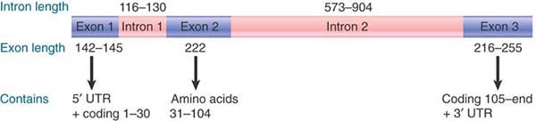
FIGURE 3.4 All functional globin genes have an interrupted structure with three exons. The lengths indicated in the figure apply to the mammalian βb-globin genes.

Introns are found at homologous positions (relative to the coding sequence) in all known active globin genes, including those of mammals, birds, and frogs. Although intron lengths vary, the first intron is always fairly short and the second is usually longer. Most of the variation in the lengths of different globin genes results from length variation in the second intron. For example, the second intron in the mouse α-globin gene is only 150 base pairs (bp) of the total 850 bp of the gene, whereas the homologous intron in the mouse major β-globin gene is 585 bp of the total 1,382 bp. The difference in length of the genes is much greater than that of their mRNAs (α-globin mRNA = 585 bases; β-globin mRNA = 620 bases).

The example of the gene for the enzyme dihydrofolate reductase (DHFR), a somewhat larger gene, is shown in FIGURE 3.5. The mammalian DHFR gene is organized into six exons that correspond to a 2,000-base mRNA. The gene itself is long because the introns are very long. In three mammal species the exons are essentially the same and the relative positions of the introns are unaltered, but the lengths of individual introns vary extensively, resulting in a variation in the length of the gene from 25 to 31 kilobases (kb).

FIGURE 3.5 Mammalian genes for DHFR have the same relative organization of rather short exons and very long introns, but vary extensively in the lengths of introns.

The globin and DHFR genes are examples of a general phenomenon: genes that share a common ancestry have similar organizations with conservation of the positions (of at least some) of the introns.

3.5 Exon Sequences Under Negative Selection Are Conserved but Introns Vary

Is a single-copy structural gene completely unique among other genes in its genome? The answer depends on how “completely unique” is defined. Considered as a whole, the gene is unique, but its exons might be related to those of other genes. As a general rule, when two genes are related, the relationship between their exons is closer than the relationship between their introns. In an extreme case, the exons of two genes might encode the same polypeptide sequence, whereas the introns are different. This situation can result from the duplication of a common ancestral gene followed by unique base substitutions in both copies, with substitutions restricted in the exons by the need to encode a functional polypeptide.

As we will see in the chapter titled Genome Sequences and Evolution, where we consider the evolution of the genome, exons can be considered basic building blocks that may be assembled in various combinations. It is possible for a gene to have some exons related to those of another gene, with the remaining exons unrelated. Usually, in such cases, the introns are not related at all. Such homologies between genes can result from duplication and translocation of individual exons.

We can plot the homology between two genes in the form of a dot matrix comparison, as in FIGURE 3.6. A dot is placed in each position that is identical in both genes. The dots form a solid line on the diagonal of the matrix if the two sequences are completely identical. If they are not identical, the line is broken by gaps that lack homology and is displaced laterally or vertically by nucleotide deletions or insertions in one or the other sequence.

FIGURE 3.6 The sequences of the mouse bβ^maj- and bβ^min-globin genes are closely related in coding regions but differ in the flanking UTRs and the long intron.

Data provided by Philip Leder, Harvard Medical School.

When the two mouse β-globin genes are compared in this way, a line of homology extends through the three exons and the small intron. The line disappears in the flanking UTRs and in the large intron. This is a typical pattern in related genes; the coding sequences and areas of introns adjacent to exons retain their similarity, but there is greater divergence in longer introns and in the regions on either side of the coding sequence.

The overall degree of divergence between two homologous exons in related genes corresponds to the differences between the polypeptides. It is mostly a result of base substitutions. In the translated regions, changes in exon sequences are constrained by selection against mutations that alter or destroy the function of the polypeptide. In other words, the exon sequences are conserved by the negative selection of individuals in which the sequences have changed (have not been conserved) to result in a phenotype that is less able to survive and produce fertile progeny. For example, if a mutation in an exon of a gene encoding a crucial enzyme destroys the function of that enzyme, those individuals that carry the mutation (if diploid, then in homozygous form) either do not survive or are otherwise severely affected. The new mutation does not persist.

Many of the preserved changes do not affect codon meanings because they change a codon into another for the same amino acid (i.e., they are synonymous substitutions). In this case, the polypeptide will not change and negative selection will not operate on the phenotype conferred by the polypeptide. Similarly, there are higher rates of change in untranslated regions of the gene (specifically, those that are transcribed to the 5′ UTR [leader] and 3′ UTR [trailer] of the mRNA).

In homologous introns, the pattern of divergence involves both changes in length (due to deletions and insertions) and base substitutions. Introns evolve much more rapidly than exons when the exons are under negative selection pressure. When a gene is compared among different species, there are instances in which its exons are homologous but its introns have diverged so much that very little homology is retained. Although mutations in certain intron sequences (branch site, splicing junctions, and perhaps other sequences influencing splicing) will be subject to selection, most intron mutations are expected to be selectively neutral.

In general, mutations occur at the same rate in both exons and introns, but exon mutations are eliminated more effectively by selection. However, because of the low level of functional constraints, introns can more freely accumulate point substitutions and other changes. Indeed, it is sometimes possible to locate exons in uncharted sequences by virtue of their conservation relative to introns (see the chapter The Content of the Genome). From this description it is all too easy to conclude that introns do not have a sequence-specific function. Genes under positive selection, however, cast a different light on the problem.

3.6 Exon Sequences Under Positive Selection Vary but Introns Are Conserved

A mutation that confers a more advantageous phenotype to an organism, relative to individuals in the same population without the mutation, can result in the preferential survival (positive selection) of that organism. Pathogenic bacteria are killed by an antibiotic, but a bacterium with a mutation that confers antibiotic resistance survives (i.e., is positively selected). Mutations conferring venom resistance to prey of venomous snakes can result in the positive selection of that prey relative to its fellows that succumb to the poison (i.e., are negatively selected). Likewise, a snake that, when confronted by a venom-resistant prey population, has a mutation that enhances the power of its venom will be positively selected. This can trigger an attack–defense cycle—an “arms race” between two protagonist species.

In such situations the pattern of exon conservation and intron variation seen in genes under negative selection can be reversed because exons evolve faster than introns. Thus, a plot similar to FIGURE 3.6 will have lines in introns and gaps in exons.

What is being conserved in introns? First, intron sequences needed for RNA splicing—the 5′ and 3′ splice sites and the branch site—are conserved (see the chapter titled RNA Splicing and Processing). In addition to these, base order has been adapted to promote the potential of the duplex DNA in the region to extrude stem-loop structures (fold potential). Thus, base order-dependent fold potential along the length of the gene (measured in negative units) is high (more negative) in introns, and low (more positive) in exons. This reciprocal relationship between substitution frequency and the contribution of base order to fold potential is a characteristic of DNA sequences under positive selection. Indeed, the low (more positive) value of fold potential in an exon provides evaluation of the extent to which it has been under positive selection, without the need to compare two sequences (the classic way of determining if selection is positive or negative).

3.7 Genes Show a Wide Distribution of Sizes Due Primarily to Intron Size and Number Variation

FIGURE 3.7 compares the organization of genes in a yeast, an insect, and mammals. In the yeast Saccharomyces cerevisiae, the majority of genes (more than 96%) are uninterrupted, and those that have exons generally have three or fewer. There are virtually no S. cerevisiae genes with more than four exons.

FIGURE 3.7 Most genes are uninterrupted in yeast, but most genes are interrupted in flies and mammals. (Uninterrupted genes have only one exon and are totaled in the leftmost column in blue.)

In insects and mammals, the situation is reversed. Only a few genes have uninterrupted coding sequences (6% in mammals). Insect genes tend to have a small number of exons, typically fewer than 10. Mammalian genes are split into more pieces and some have more than 60 exons. Approximately 50% of mammalian genes have more than 10 introns. If we examine the effect of intron number variation on the total size of genes, we see in FIGURE 3.8 that there is a striking difference between yeast and multicellular eukaryotes. The average yeast gene is 1.4 kb long, and very few are longer than 5 kb. The predominance of interrupted genes in multicellular eukaryotes, however, means that the gene can be much larger than the sum total of the exon lengths. Only a small percentage of genes in flies or mammals are shorter than 2 kb, and most have lengths between 5 kb and 100 kb. The average human gene is 27 kb long. The gene encoding Caspr2, with a length of 2,300 kb, is the longest known human gene (it encompasses nearly 1.5% of the entire length of human chromosome 7!).

FIGURE 3.8 Yeast genes are short, but genes in flies and mammals have a dispersed bimodal distribution extending to very long sizes.

The switch from largely uninterrupted to largely interrupted genes seems to have occurred with the evolution of multicellular eukaryotes. In fungi other than S. cerevisiae, the majority of genes are interrupted, but they have a relatively small number of exons (fewer than 6) and are fairly short (less than 5 kb). In the fruit fly, gene sizes have a bimodal distribution—many are short but some are quite long. With this increase in the length of the gene due to the increased number of introns, the correlation between genome size and organism complexity becomes weak.

FIGURE 3.9 shows that exons encoding stretches of protein tend to be fairly small. In multicellular eukaryotes, the average exon codes for about 50 amino acids, and the general distribution is consistent with the hypothesis that genes have evolved by the gradual addition of exon units that encode short, functionally independent protein domains (see the Genome Sequences and Evolution chapter). There is no significant difference in the average size of exons in different multicellular eukaryotes, although the size range is smaller in vertebrates for which there are few exons longer than 200 bp. In yeast, there are some longer exons that represent uninterrupted genes for which the coding sequence is intact. There is a tendency for exons containing untranslated 5′ and 3′ regions to be longer than those that encode proteins.

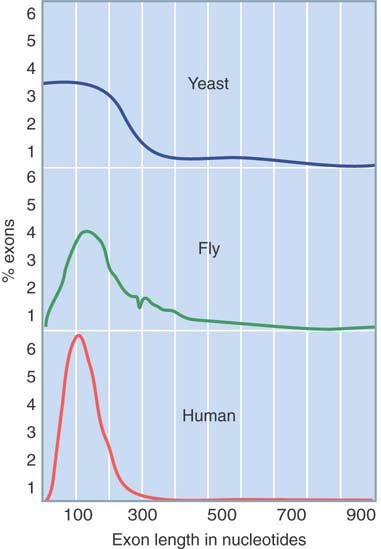
FIGURE 3.9 Exons encoding polypeptides are usually short.

FIGURE 3.10 shows that introns vary widely in size among multicellular eukaryotes. (Note that the scale of the x-axis differs from that of Figure 3.9.) In worms and flies, the average intron is no longer than the exons. There are no very long introns in worms, but flies contain many. In vertebrates, the size distribution is much wider, extending from approximately the same length as the exons (less than 200 bp) up to 60 kb in extreme cases. (Some fish, such as fugu [pufferfish], have compressed genomes with shorter introns and intergenic regions than mammals have.)

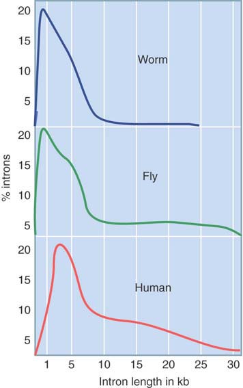
FIGURE 3.10 Introns range from very short to very long.

Very long genes are the result of very long introns, not the result of encoding longer products. There is no correlation between total gene size and total exon size in multicellular eukaryotes, nor is there a good correlation between gene size and number of exons. The size of a gene is therefore determined primarily by the lengths of its individual introns. In mammals and insects, the “average” gene is approximately 5 times that of the total length of its exons.

3.8 Some DNA Sequences Encode More Than One Polypeptide

Many structural genes consist of a sequence that encodes a single polypeptide, although the gene can include noncoding regions at both ends and introns within the coding region. However, there are some cases in which a single sequence of DNA encodes more than one polypeptide.

In one simple example, a single DNA sequence can have two alternative start codons in the same reading frame (see FIGURE 3.11). Thus, under different conditions one or the other of the start codons might be used, allowing the production of either a short form of the polypeptide or a full-length form, where the short form is the last portion of the full-length form.

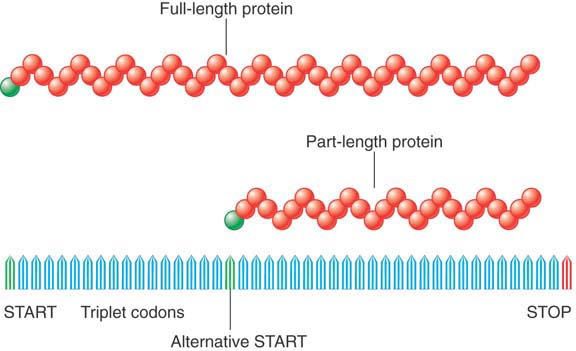
FIGURE 3.11 Two proteins can be generated from a single gene by starting (or terminating) expression at different points.

An actual overlapping gene occurs when the same sequence of DNA encodes two nonhomologous proteins because it uses more than one reading frame. Usually, a coding DNA sequence is read in only one of the three potential reading frames. In some viral and mitochondrial genes, however, there is some overlap between two adjacent genes that are read in different reading frames, as illustrated in FIGURE 3.12. The length of overlap is usually short, so that most of the DNA sequence encodes a unique polypeptide sequence.

FIGURE 3.12 Two genes might overlap by reading the same DNA sequence in different frames.

In some cases, genes can be nested. This occurs when a complete gene is found within the intron of a larger “host” gene. Nested genes often lie on the strand opposite that of the host gene.

In some genes there are switches in the pathway for splicing the exons that result in alternative patterns of gene expression. A single gene might generate a variety of mRNA products that differ in their exon content. Certain exons might be optional; in other words, they might be included or spliced out. There also might be a pair of exons treated as mutually exclusive—one or the other is included in the mature transcript, but not both. The alternative proteins have one part in common and one unique part.

In some cases, the alternative means of expression do not affect the sequence of the polypeptide. For example, changes that affect the 5′ UTR or the 3′ UTR might have regulatory consequences, but the same polypeptide is made. In other cases, one exon is substituted for another, as in FIGURE 3.13. In this example, the polypeptides produced by the two mRNAs contain sequences that overlap extensively, but are different within the alternatively spliced region. The 3′ half of the troponin T gene of rat muscle contains five exons, but only four are used to construct an individual mRNA. Three exons (W, X, and Z) are included in all mRNAs. However, in one alternative splicing pattern, the α exon is included between X and Z, whereas in the other pattern it is replaced by the β exon. The α and β forms of troponin T therefore differ in the sequence of the amino acids between W and Z, depending on which of the alternative exons (α or β) is used. Either one of the α and β exons can be used in an individual mRNA, but both cannot be used in the same mRNA.

FIGURE 3.13 Alternative splicing generates the a and b variants of troponin T.

FIGURE 3.14 shows that alternative splicing can lead to the inclusion of an exon in some mRNAs, whereas it leaves it out of others. A single primary transcript can be spliced in either of two ways. In the first (more standard) pathway, two introns are spliced out and the three exons are joined together. In the second pathway, the second exon is excluded as if a single large intron is spliced out. This intron consists of intron 1 + exon 2 + intron 2. In effect, exon 2 has been treated in this pathway as if it were part of a single intron. The pathways produce two polypeptides that are the same at their ends, but one has an additional sequence in the middle. (Other types of combinations that are produced by alternative splicing are discussed in the RNA Splicing and Processing chapter.)

FIGURE 3.14 Alternative splicing uses the same pre-mRNA to generate mRNAs that have different combinations of exons.

Sometimes two alternative splicing pathways operate simultaneously, with a certain proportion of the primary RNA transcripts being spliced in each way. However, sometimes the pathways are alternatives that are expressed under different conditions; for example, one in one cell type and one in another cell type.

So, alternative (or differential) splicing can generate different polypeptides with related sequences from a single stretch of DNA. It is curious that the multicellular eukaryotic genome is often extremely large with long genes that are often widely dispersed along a chromosome, but at the same time there might be multiple products from a single locus. Due to alternative splicing, there are about 15% more polypeptides than genes in flies and worms, but it is estimated that the majority of human genes are alternatively spliced (see the chapter titled Genome Sequences and Evolution).

3.9 Some Exons Correspond to Protein Functional Domains

The issue of the evolution of interrupted genes is more fully considered in the Genome Sequences and Evolution chapter. If proteins evolve by recombining parts of ancestral proteins that were originally separate, the accumulation of protein domains is likely to have occurred sequentially, with one exon added at a time. Each addition would need to improve upon the advantages of prior additions in a sequence of positive selection events. Are the different function-encoding segments from which these genes might have originally been pieced together reflected in their present structures? If a protein sequence were randomly interrupted, sometimes the interruption would intersect a domain and sometimes it would lie between domains. If we can associate the functional domains of current proteins with the individual exons of the corresponding genes, this would suggest selective interdomain interruptions rather than random ones.

In some cases, there is a clear relationship between the structures of a gene and its protein product, but these might be special cases. The example par excellence is provided by the immunoglobulin (antibody) proteins—an extracellular system for self-/nonself-discrimination that aids in the elimination of foreign pathogens. Immunoglobulins are encoded by genes in which every exon corresponds exactly to a known functional protein domain. Banks of alternate sequence domains are tapped so that each cell acquires the ability to secrete a cell-specific immunoglobulin with distinctive binding capacity for a foreign antigen that the organism might someday encounter again (see the chapter titled Somatic DNA Recombination and Hypermutation in the Immune System). FIGURE 3.15 compares the structure of an immunoglobulin with its gene.

FIGURE 3.15 Immunoglobulin light chains and heavy chains are encoded by genes whose structures (in their expressed forms) correspond to the distinct domains in the protein. Each protein domain corresponds to an exon; introns are numbered I1 to I5.

An immunoglobulin is a tetramer of two light chains and two heavy chains that covalently bond to generate a protein with several distinct domains. Light chains and heavy chains differ in structure, and there are several types of heavy chains. Each type of chain is produced from a gene that has a series of exons corresponding to the structural domains of the protein.

In many instances, some of the exons of a gene can be identified with particular functions. In secretory proteins, such as insulin, the first exon that encodes the N-terminal region of the polypeptide often specifies a signal sequence needed for transfer across a membrane.

The view that exons are the functional building blocks of genes is supported by cases in which two genes can share some related exons but also have unique exons. FIGURE 3.16 summarizes the relationship between the receptor for human plasma low-density lipoprotein (LDL) and other proteins. The LDL receptor gene has a series of exons related to the exons of the epidermal growth factor (EGF) precursor gene and another series of exons related to those of the blood protein complement factor C9. Apparently, the LDL receptor gene evolved by the assembly of modules for its various functions. These modules are also used in different combinations in other proteins.

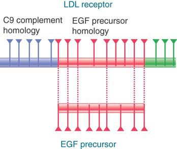
FIGURE 3.16 The LDL receptor gene consists of 18 exons, some of which are related to EGF precursor exons and some of which are related to the C9 blood complement gene. Triangles mark the positions of introns.

Exons tend to be fairly small—around the size of the smallest polypeptide that can assume a stable folded structure (approximately 20 to 40 residues). It might be that proteins were originally assembled from rather small modules. Each individual module need not correspond to a current function; several modules could have combined to generate a new functional unit. Larger genes tend to have more exons, which is consistent with the view that proteins acquire multiple functions by successively adding appropriate modules.

This suggestion might explain another aspect of protein structure: it appears that the sites represented at exon-intron boundaries often are located at the surface of a protein. As modules are added to a protein, the connections—at least of the most recently added modules—could tend to lie at the surface.

3.10 Members of a Gene Family Have a Common Organization

Many genes in a multicellular eukaryotic genome are related to others in the same genome, either in series (nonallelic) or in parallel (allelic). A gene family is defined as a group of genes that encode related or identical products as a result of gene duplication events. After the first duplication event, the two copies are identical, but then they diverge as different mutations accumulate in them. Further duplications and divergences extend the family. The globin genes are an example of a family that can be divided into two subfamilies (α globin and β globin), but all of its members have the same basic structure and function (see the Genome Sequences and Evolution chapter). In some cases, we can find genes that are more distantly related but that still can be recognized as having common ancestry. Such a group of gene families is called a superfamily.

A fascinating case of evolutionary conservation is presented by the α and β globins and two other proteins related to them. Myoglobin is a monomeric oxygen-binding protein in animals. Its amino acid sequence suggests a common (though ancient) origin with α and β globins. Leghemoglobins are oxygen-binding proteins present in legume plants; like myoglobin, they are monomeric and share a common origin with the other heme-binding proteins. Together, the globins, myoglobins, and leghemoglobins make up the globin superfamily—a set of gene families all descended from an ancient common ancestor.

Both α- and β-globin genes have three exons and two introns in conserved positions (see Figure 3.4). The central exon represents the heme-binding domain of the globin chain. There is a single myoglobin gene in the human genome and its structure is essentially the same as that of the globin genes. The conserved three-exon structure therefore predates the common ancestor of the myoglobin and globin genes.

Leghemoglobin genes contain three introns, the first and last of which are homologous to the two introns in the globin genes. This remarkable similarity suggests an exceedingly ancient origin for the interrupted structure of heme-binding proteins, as illustrated in FIGURE 3.17. The central intron of leghemoglobin separates two exons that together encode the sequence corresponding to the single central exon in globin; the functional heme-binding domain is split into two by an intron. Could the central exon of the globin gene have been derived by a fusion of two central exons in the ancestral gene? Or, is the single central exon the ancestral form? In this case, an intron must have been inserted into it early in plant evolution.

FIGURE 3.17 The exon structure of globin genes corresponds to protein function, but leghemoglobin has an extra intron in the central domain.

Orthologous genes, or orthologs, are genes that are homologous (homologs) due to speciation; in other words, they are related genes in different species. Comparison of orthologs that differ in structure might provide information about their evolution. An example is insulin. Mammals and birds have only one gene for insulin, except for rodents, which have two. FIGURE 3.18 illustrates the structures of these genes.

FIGURE 3.18 The rat insulin gene with one intron evolved by loss of an intron from an ancestor with two introns.

We use the principle of parsimony in comparing the organization of orthologous genes by assuming that a common feature predates the evolutionary separation of the two species. In chickens, the single insulin gene has two introns; one of the two homologous rat genes has the same structure. The common structure implies that the ancestral insulin gene had two introns. However, because the second rat gene has only one intron, it must have evolved by a gene duplication in rodents that was followed by the precise removal of one intron from one of the homologs.

The organizations of some orthologs show extensive discrepancies between species. In these cases, there must have been extensive deletion or insertion of introns during evolution. A well characterized case is that of the actin genes. The common features of actin genes are an untranslated leader of fewer than 100 bases, a coding region of about 1,200 bases, and a trailer of about 200 bases. Most actin genes have introns, and their positions can be aligned with regard to the coding sequence (except for a single intron sometimes found in the leader).

FIGURE 3.19 shows that almost every actin gene is different in its pattern of intron positions. Among all the genes being compared, introns occur at 19 different sites. However, the range of intron number per gene is zero to six. How did this situation arise? If we suppose that the ancestral actin gene had introns, and that all current actin genes are related to it by loss of introns, different introns have been lost in each evolutionary branch. Probably some introns have been lost entirely, so the ancestral gene could well have had 20 introns or more. The alternative is to suppose that a process of intron insertion continued independently in the different lineages.

FIGURE 3.19 Actin genes vary widely in their organization. The sites of introns are indicated by dark boxes. The bar at the top summarizes all the intron positions among the different orthologs.

Whether introns were present in actin genes early or late, there appears to have been no consistent influence from actin protein domains or subdomains as to where introns should be located. On the other hand, when exons are under negative selection (resulting in homology conservation), in-series recombination between members of an expanding gene family (that could cause a contraction in family size) would be decreased by intron diversification (resulting in loss of some homology), and introns would come to reside where this could best be achieved.

Alleles would have similar exons and introns, so in-parallel interallelic recombination (as in meiosis) would be unimpaired until speciation occurred—a process that could be accompanied by intron relocations. The relationships between the intron locations among different species could then be used to construct a phylogenetic tree illustrating the evolution of the actin gene.

The relationship between individual exons and functional protein domains is somewhat erratic. In some cases, there is a clear one-to-one relationship; in others, no pattern can be discerned. One possibility is that the removal of introns has fused the previously adjacent exons. This means that the intron must have been precisely removed without changing the integrity of the coding region. An alternative is that some introns arose by insertion into an exon encoding a single domain. Together with the variations that we see in exon placement in cases such as the actin genes, the conclusion is that intron positions can evolve.

The correspondence of at least some exons with protein domains and the presence of related exons in different proteins leave no doubt that the duplication and juxtaposition of exons have played important roles in evolution. It is possible that the number of ancestral exons—from which all proteins have been derived by duplication, variation, and recombination—could be relatively small, perhaps as little as a few thousand. The idea that exons are the building blocks of new genes is consistent with the “introns early” model for the origin of genes encoding proteins (see the Genome Sequences and Evolution chapter).

3.11 There Are Many Forms of Information in DNA

The term genetic information can include all information that passes “vertically” through the germ line, not just genic information. The word “gene” and its adjective “genic” have different meanings in different contexts, but in most circumstances there is little confusion when context is considered. For situations in which a sequence of DNA is responsible for production of one particular polypeptide, current usage regards the entire sequence of DNA—from the first point represented in the messenger RNA to the last point corresponding to its end—as comprising the “gene”: exons, introns, and all.

When sequences encoding polypeptides overlap or have alternative forms of expression, we can reverse the usual description of the gene. Instead of saying “one gene–one polypeptide,” we can describe the relationship as “one polypeptide–one gene.” So we regard the sequence involved in production of the polypeptide (including introns and exons) as constituting the gene, while recognizing that part of this same sequence also belongs to the gene of another polypeptide. This allows the use of descriptions such as “overlapping” or “alternative” genes.

We can now see how far we have come from the one gene–one enzyme hypothesis of the 20th century. The driving question at that time was the nature of the gene. It was thought that genes represented “ferments” (enzymes), but what was the fundamental nature of ferments? After it was discovered that most genes encode proteins, the paradigm became fixed as the concept that every genetic unit functions through the synthesis of a particular protein. Either directly or indirectly, protein-encoding pressure was responsible for what we can now refer to as the conventional phenotype. We now recognize that genetic units encoding polypeptides can also include information corresponding to the genome phenotype, manifestations of which include fold pressure, purine-loading (AG) pressure, and GC pressure. There can be conflict between different pressures, such as competition for space in the gamete that will transfer genomic information to the next generation. For example, a protein might function most efficiently with the basic amino acid lysine (codon AAA) in a certain position, but GC pressure might require the substitution of another basic amino acid, such as arginine (codon CGG). Alternatively, fold pressure might require the corresponding nucleic acid to fold into a stem-loop structure in which CCG would pair with the antiparallel arginine codon. A lysine codon in this position would disrupt the structure, so again a less efficient polypeptide would need to suffice.

The conventional phenotype, however, remains the central paradigm of molecular biology: a genic DNA sequence either directly encodes a particular polypeptide or is adjacent to the segment that actually encodes that polypeptide. How far does this paradigm take us beyond explaining the basic relationship between genes and proteins?

The development of multicellular organisms required the use of different genes to generate the different cell phenotypes of each tissue. The expression of genes is determined by a regulatory network that takes the form of a cascade. Expression of the first set of genes at the beginning of embryonic development leads to expression of the genes involved in the next stage of development, which in turn leads to a further stage, and so on, until all of the tissues of the adult are formed and functioning. The molecular nature of this regulatory network is still under investigation, but we see that it consists of genes that encode products (often protein, but sometimes RNA) that can influence the expression of other genes.

Although such a series of interactions is almost certainly the means by which the developmental program is executed, we can ask whether it is entirely sufficient. One specific question concerns the nature and role of positional information. We know that all parts of a fertilized egg are not equal; one of the features responsible for development of different tissue parts from different regions of the egg is location of information (presumably specific macromolecules) within the cell.

We do not fully understand how these particular regions are formed, though particular examples have been well studied (see the mRNA Stability and Localization chapter). We assume, however, that the existence of positional information in the egg leads to the differential expression of genes in the cells making up the tissues formed from these regions. This leads to the development of the adult organism, which in the next generation leads to the development of an egg with the appropriate positional information.

This possibility of positional information suggests that some information needed for development of the organism is contained in a form that we cannot directly attribute to a sequence of DNA (although the expression of particular sequences might be needed to perpetuate the positional information). Put in a more general way, we might ask the following: If we have the entire sequence of DNA comprising the genome of some organism and interpret it in terms of proteins and regulatory regions, could we in principle construct an organism (or even a single living cell) by controlled expression of the proper genes?

After tissues and organs have developed, they not only must be maintained but also protected against potential pathogens. Groups of variable genes have diversified in the germ line, and continue to diversify somatically, to allow multicellular organisms to (1) respond extracellularly by the synthesis of immunoglobulin antibodies directed against pathogens, and (2) “remember” past pathogens so that future responses will be faster and stronger (immunological memory; see the chapter titled Somatic DNA Recombination and Hypermutation in the Immune System). Should it escape such extracellular defenses, though, the nucleic acid of a pathogenic virus could gain entry to cells and intracellular defenses would be needed.

We know that in bacteria infected by bacteriophages (see the chapter titled Phage Strategies), host defenses include rapid local or genome-wide transcription of DNA (which has been documented in eukaryotes in response to environmental insult or infection) to produce “antisense” transcripts that are capable of base-pairing with pathogen “sense” transcripts to form double-stranded RNAs. These RNAs then act as an alarm signal to trigger secondary defenses (see the example of bacterial CRISPRs discussed in the Regulatory RNA chapter). The host could store a “memory” of previous intracellular invaders by converting some pathogen transcripts into DNA through reverse transcription and inserting them into its genome in an inactive form for future rapid transcription of antisense RNAs in times of active infection by that pathogen. Thus, some pathogen nucleic acid might enter the germline “horizontally” (within a generation) and the parental memory of the pathogen could subsequently be transferred “vertically” to offspring. The diversity of some elements found within introns and extragenic DNA (see the chapter titled Transposable Elements and Retroviruses) could in part reflect such past pathogen attacks. There is recent evidence of such inherited antiviral immunity in several animal and plant species.

Summary

Most eukaryotic genomes contain genes that are interrupted by intron sequences. The proportion of interrupted genes is low in some fungi, but few genes are uninterrupted in multicellular eukaryotes. The size of a gene is determined primarily by the lengths of its introns. The range of gene sizes in mammals is generally from 1 to 100 kb, but there are some that are even larger.
Introns are found in all classes of eukaryotic genes, both those encoding protein products and those encoding independently functioning RNAs. The structure of an interrupted gene is the same in all tissues: Exons are spliced together in RNA in the same order as they are found in DNA, and the introns, which usually have no coding function, are removed from RNA by splicing. Some genes are expressed by alternative splicing patterns, in which a particular sequence is removed as an intron in some situations but retained as an exon in others.
Often, when the organizations of orthologous genes are compared, the positions of introns are conserved. In genes under negative selection pressure, intron sequences vary—and might even appear unrelated—although exon sequences remain closely related. We can use this conservation of exons, which allows the conservation of important phenotypic characters, to identify related genes in different species. In genes under positive selection pressure, however, exon sequences vary, although intron sequences can remain more similar. This conservation of introns relates to characters corresponding to the genome phenotype, such as fold pressure, which might relate to error correction in DNA.
Some genes share only some of their exons with other genes, suggesting that they have been assembled by addition of exons representing functional “modular units” of the protein. Such modular exons might have been incorporated into a variety of different proteins and sometimes correspond to functional domains of those proteins. The idea that genes have been assembled by sequential addition of exons is consistent with the hypothesis that introns were present in the genes of ancestral organisms, thus facilitating the assembly process. We can explain some of the relationships between homologous genes by loss of introns from the ancestral genes, with different introns being lost in different lines of descent.

References

3.1 Introduction

Reviews

Crick, F. (1979). Split genes and RNA splicing. Science 204, 264–271.
Harris, H. (1994). An RNA heresy in the fifties. Trends Biochem. Sci. 19, 303–305.
Hong, X., Schofield, D. G., and Lynch, M. (2006). Intron size, abundance, and distribution within untranslated regions of genes. Mol. Biol. Evol. 2, 2392–2404.

Research

Glover, D. M., and Hogness, D. S. (1977). A novel arrangement of the 8S and 28S sequences in a repeating unit of D. melanogaster rDNA. Cell 10, 167–176.
Scherrer, K., et al. (1970). Nuclear and cytoplasmic messenger-like RNAs and their relation to the active messenger RNA in polyribosomes of HeLa cells. Cold Spring Harb. Symp. Quant. Biol. 35, 539–554.

3.2 An Interrupted Gene Has Exons and Introns

Review

Forsdyke, D. R. (2011). Exons and introns. In Evolutionary Bioinformatics, 2nd ed. New York: Springer, pp. 249–266. (See also http://post.queensu.ca/~forsdyke/introns.htm.)

3.3 Exon and Intron Base Compositions Differ

Reviews

Forsdyke, D. R., and Bell, S. J. (2004). Purine-loading, stem-loops, and Chargaff’s second parity rule: a discussion of the application of elementary principles to early chemical observations. Applied Bioinformatics 3, 3–8. (See http://post.queensu.ca/~forsdyke/bioinfo5.htm.)
Forsdyke, D. R., and Mortimer, J. R. (2000). Chargaff’s legacy. Gene. 261, 127–137. (See http://post.queensu.ca/~forsdyke/bioinfo2.htm.)

Research

Babak, T., Blencowe, B. J., and Hughes, T. R. (2007). Considerations in the identification of functional RNA structural elements in genomic alignments. BMC. Bioinf. 8, article number 33.
Bechtel, J. M., et al. (2008). Genomic mid-range inhomogeneity correlates with an abundance of RNA secondary structure. BMC. Genomics. 9, article number 284.
Bultrini, E., et al. (2003). Pentamer vocabularies characterizing introns and intron-like intergenic tracts from Caenorhabditis elegans and Drosophila melanogaster. Gene. 304, 183–192.
Ko, C. H., et al. (1998). U-richness is a defining feature of plant introns and may function as an intron recognition signal in maize. Plant. Mol. Biol. 36, 573–583.
Zhang, C., Li, W. H., Krainer, A. R., and Zhang, M. Q. (2008). RNA landscape of evolution for optimal exon and intron discrimination. Proc. Natl. Acad. Sci. USA 105, 5797–5802.

3.4 Organization of Interrupted Genes May Be Conserved

Review

Fedoroff, N. V. (1979). On spacers. Cell 16, 697–710.

Research

Berget, S. M., Moore, C., and Sharp, P. (1977). Spliced segments at the 5′ terminus of adenovirus 2 late mRNA. Proc. Natl. Acad. Sci. USA 74, 3171–3175.
Chow, L. T., Gelinas, R. E., Broker, T. R., and Roberts, R. J. (1977). An amazing sequence arrangement at the 5′ ends of adenovirus 2 mRNA. Cell 12, 1–8.
Jeffreys, A. J., and Flavell, R. A. (1977). The rabbit β-globin gene contains a large insert in the coding sequence. Cell 12, 1097–1108.

3.6 Exon Sequences Under Positive Selection Vary but Introns Are Conserved

Forsdyke, D. R. (1995). Conservation of stem-loop potential in introns of snake venom phospholipase A2 genes: an application of FORS-D analysis. Mol. Biol. Evol. 12, 1157–1165.
Forsdyke, D. R. (1995). Reciprocal relationship between stem-loop potential and substitution density in retroviral quasispecies under positive Darwinian selection. J. Mol. Evol. 41, 1022–1037. (See http://post.queensu.ca/~forsdyke/hiv01.htm.)
Forsdyke, D. R. (1996). Stem-loop potential in MHC genes: a new way of evaluating positive Darwinian selection. Immunogenetics 43, 182–189.

3.7 Genes Show a Wide Distribution of Sizes Due Primarily to Intron Size and Number Variation

Hawkins, J. D. (1988). A survey of intron and exon lengths. Nucleic. Acids. Res. 16, 9893–9905.
Naora, H., and Deacon, N. J. (1982). Relationship between the total size of exons and introns in protein-coding genes of higher eukaryotes. Proc. Natl. Acad. Sci. USA 79, 6196–6200.

3.8 Some DNA Sequences Encode More Than One Polypeptide

Review

Chen, M., and Manley, J. L. (2009). Mechanisms of alternative splicing regulation: insights from molecular and genomics approaches. Nat. Rev. Mol. Cell. Biol. 10, 741–754.

Research

Pan, Q., et al. (2008). Deep surveying of alternative splicing complexity in the human transcriptome by high-throughput sequencing. Nature Genetics 40, 1413–1415.
Sultan, M., et al. (2008). A global view of gene activity and alternative splicing by deep sequencing of the human transcriptome. Science 321, 956–960.

3.9 Some Exons Correspond to Protein Functional Domains

Reviews

Blake, C. C. (1985). Exons and the evolution of proteins. Int. Rev. Cytol. 93, 149–185.
Doolittle, R. F. (1985). The genealogy of some recently evolved vertebrate proteins. Trends Biochem. Sci. 10, 233–237.

3.10 Members of a Gene Family Have a Common Organization

Review

Dixon, B., and Pohajdek, B. (1992). Did the ancestral globin gene of plants and animals contain only two introns? Trends Biochem. Sci. 17, 486–488.

Research

Matsuo, K., et al. (1994). Short introns interrupting the Oct-2 POU domain may prevent recombination between POU family members without interfering with potential POU domain ‘shuffling’ in evolution. Biol. Chem. Hopp-Seyler 375, 675–683.
Weber, K., and Kabsch, W. (1994). Intron positions in actin genes seem unrelated to the secondary structure of the protein. EMBO. J. 13, 1280–1286.

3.11 There Are Many Forms of Information in DNA

Reviews

Barrangou, R., et al. (2007). CRISPR provides acquired resistance against viruses in prokaryotes. Science 315, 1709–1712.
Bernardi, G., and Bernardi, G. (1986). Compositional constraints and genome evolution. J. Mol. Evol. 24, 1–11.
Forsdyke, D. R. (2011). Evolutionary Bioinformatics, 2nd ed. New York: Springer.
Forsdyke, D. R., Madill, C. A., and Smith, S. D. (2002). Immunity as a function of the unicellular state: implications of emerging genomic data. Trends Immunol. 23, 575–579. (See http://post.queensu.ca/~forsdyke/theorimm.htm.)
Jeffares, D. C, Penkett, C. J., and Bähler, J. (2008). Rapidly regulated genes are intron poor. Trends in Genetics 24, 375–378.

Research

Bertsch, C., Beuve, M., Dolja, V. V., Wirth, M., Pelsy, F., Herrbach, E., and Lemaire, O. (2009). Retention of the virus-derived sequences in the nuclear genome of grapevine as a potential pathway to virus resistance. Biology Direct 4, 21.
Flegel, T. W. (2009). Hypothesis for heritable, antiviral immunity in crustaceans and insects. Biology Direct 4, 32.
Saleh, M. C, Tassetto, M., van Rij, R. P., Goic, B., Gausson, V., Berry, B., Jacquier, C., Antoniewski, C., and Andino, R. (2009). Antiviral immunity in Drosophila requires systemic RNA interference spread. Nature 458, 346–350.