
Top texture: © Laguna Design / Science Source;
Chapter 4: The Content of the Genome
Chapter Opener: © cdascher/Getty Images.
4.1 Introduction
One key question about any genome is how many genes it contains. However, there’s an even more fundamental question: “What is a gene?” Clearly, genes cannot be defined solely as a sequence of DNA that encodes a polypeptide, because many genes encode multiple polypeptides and many encode RNAs that serve other functions. Given the variety of RNA functions and the complexities of gene expression, it seems prudent to focus on the gene as a unit of transcription. However, large areas of chromosomes previously thought to be devoid of genes now appear to be extensively transcribed, so at present the definition of a “gene” is a moving target.
We can attempt to characterize both the total number of genes and the number of protein-coding genes at four levels, which correspond to successive stages in gene expression:
The genome is the complete set of genes of an organism. Ultimately, it is defined by the complete DNA sequence, although as a practical matter it might not be possible to identify every gene unequivocally solely on the basis of sequence.
The transcriptome is the complete set of genes expressed under particular conditions. It is defined in terms of the set of RNA molecules present in a single cell type, a more complex assembly of cells, or a complete organism. Because some genes generate multiple messenger RNAs (mRNAs), the transcriptome is likely to be larger than the actual number of genes in the genome. The transcriptome includes noncoding RNAs such as transfer RNAs (tRNAs), ribosomal RNAs (rRNAs), microRNAs (miRNAs), and others (see the chapters titled Noncoding RNA and Regulatory RNA), as well as mRNAs.
The proteome is the complete set of polypeptides encoded by the whole genome or produced in any particular cell or tissue. It should correspond to the mRNAs in the transcriptome, although there can be differences of detail reflecting changes in the relative abundance or stabilities of mRNAs and proteins. There might also be posttranslational modifications to proteins that allow more than one protein to be produced from a single transcript (this is called protein splicing; see the Catalytic RNA chapter).
Proteins can function independently or as part of multiprotein or multimolecular complexes, such as holoenzymes and metabolic pathways where enzymes are clustered together. The RNA polymerase holoenzyme (see the Prokaryotic Transcription chapter) and the spliceosome (see the RNA Splicing and Processing chapter) are two examples. If we could identify all protein–protein interactions, we could define the total number of independent complexes of proteins. This is sometimes referred to as the interactome.
The maximum number of polypeptide-encoding genes in the genome can be identified directly by characterizing open reading frames (ORFs). Large-scale analysis of this nature is complicated by the fact that interrupted genes might consist of many separated ORFs, and alternative splicing can result in the use of variously combined portions of these ORFs. We do not necessarily have information about the functions of the polypeptide products—or indeed proof that they are expressed at all—so this approach is restricted to defining the potential of the genome. However, it is presumed that any conserved ORF is likely to be expressed.
Another approach is to define the number of genes directly in terms of the transcriptome (by directly identifying all the RNAs) or proteome (by directly identifying all the polypeptides). This gives an assurance that we are dealing with bona fide genes that are expressed under known circumstances. It allows us to ask how many genes are expressed in a particular tissue or cell type, what variation exists in the relative levels of expression, and how many of the genes expressed in one particular cell are unique to that cell or are also expressed elsewhere. In addition, analysis of the transcriptome can reveal how many different mRNAs (e.g., mRNAs containing different combinations of exons) are generated from a particular gene.
Also, we might ask whether a particular gene is essential: What is the phenotypic effect of a null mutation in that gene? If a null mutation is lethal or the organism has a clear defect, we can conclude that the gene is essential or at least beneficial. However, the functions of some genes can be eliminated without apparent effect on the phenotype. Are these genes really dispensable, or does a selective disadvantage result from the absence of the gene, perhaps in other circumstances or over longer periods of time? In some cases, the absence of the functions of these genes could be offset by a redundant mechanism, such as a gene duplication, providing a backup for an essential function.
4.2 Genome Mapping Reveals That Individual Genomes Show Extensive Variation
Defining the contents of a genome essentially means mapping and sequencing the genetic loci found on the organism’s chromosome(s). Prior to the modern technological ease and low cost of DNA sequencing, there were several low-resolution genome mapping techniques. A linkage map shows the distance between loci in units based on recombination frequencies; it is limited by its dependence on the observation of recombination between variable markers that are either directly visible (e.g., phenotypic traits) or that can otherwise be visualized (e.g., by electrophoresis). A restriction map is constructed by cutting DNA into fragments with restriction enzymes and measuring the physical distances, in terms of the length of DNA in base pairs (determined by migration on an electrophoretic gel) between the cut sites.
Today, a genomic map is constructed by sequencing the DNA of the genome. From the sequence, we can identify genes and the distances between them. By analyzing the protein-coding potential of a sequence of the DNA, we can hypothesize about its function. The basic assumption is that natural selection prevents the accumulation of deleterious mutations in sequences that encode functional products. Reversing the argument, we can assume that an intact coding sequence with accompanying transcription signals is likely to produce a functional polypeptide.
By comparing a wild-type DNA sequence with that of a mutant allele, researchers can determine the nature of a mutation and its exact location in the sequence. This provides a way to determine the relationship between the linkage map (based entirely on variable sites) and the physical map (based on, or even comprising, the sequence of DNA).
Researchers use similar techniques to identify and sequence genes and to map the genome, although there is, of course, a difference of scale. In each case, the approach is to characterize a series of overlapping fragments of DNA that can be connected into a continuous map. The crucial feature is that each segment is identified as adjacent to the next segment on the map by the overlap between them, so that we can be sure no segments are missing. This principle is applied both at the level of assembling large fragments into a map and in connecting the sequences that make up the fragments.
The original Mendelian view of the genome classified alleles as either wild type or mutant. Subsequently, the existence of multiple alleles for a gene in a population has been recognized, each with a different effect on the phenotype. In some cases, it might not even be appropriate to define any one allele as wild type.
The coexistence of multiple alleles at a locus in a population is called genetic polymorphism. Any site at which multiple alleles exist as stable components of the population is by definition polymorphic. A locus is usually defined as polymorphic if two or more alleles are present at a frequency of more than 1% in the population. Human eye color is a good example of phenotypic polymorphism resulting from underlying genetic polymorphism. There is no single “normal” eye color; many different colors are found among different individuals, with little or no differences in visual function among them.
What is the basis for the polymorphism among the varying alleles? They possess different mutations that might alter their product’s function, thus producing changes in phenotype. The population dynamics of these different alleles are partly determined by their selective effects on phenotype. If we compare the restriction maps or the DNA sequences of these alleles, they will also be polymorphic in the sense that each map or sequence will be different from the others.
Although not evident from the phenotype, the wild type might itself be polymorphic. Multiple versions of the wild-type allele can be distinguished by differences in sequence that do not affect their function and therefore do not produce phenotypic variants. A population can have extensive polymorphism at the level of the genotype. Many different sequence variants can exist at a particular locus; some of them are evident because they affect the phenotype, but others are “hidden” because they have no visible effect. These mutant alleles are usually selectively neutral, with their population dynamics mainly a result of random genetic drift.
There can be a variety of changes at a locus, including those that change the DNA sequence but do not change the sequence of the polypeptide product, those that change the polypeptide sequence without changing its function, those that result in polypeptides with different functions, and those that result in altered polypeptides that are nonfunctional.
When alleles of the same locus are compared, a difference in a single nucleotide is called a single nucleotide polymorphism (SNP). On average, one SNP occurs for approximately every 1,330 bases in the human genome. Defined by SNPs, every human being is unique. SNPs can be detected by direct comparisons of sequences from different individuals.
One aim of genetic mapping is to obtain a catalog of common variants. The observed frequency of SNPs per genome predicts that, in the human population as a whole (considering the genomes of all living human individuals), there should be more than 10 million SNPs that occur at a frequency of more than 1% (i.e., are polymorphic). (As of the end of 2015, more than 100 million human SNPs have been identified, though most of these do not fit the definition of polymorphic.)
The sequencing of complete individual genomes is now possible and allows the assessment of individual DNA-level variations, both neutral SNPs and those linked to diseases or disease susceptibilities. Although the sequencing of “celebrity” genomes (e.g., those of James Watson and Craig Venter) receive more press coverage, rapid genome sequencing of anonymous individuals is potentially more informative. Hundreds of individual human genomes of all major racial groups have now been sequenced, including those of Denisovans (a Paleolithic Homo species that lived more than 30,000 years ago) and Neanderthals (more than 25,000 years old). The 1,000 Genomes Project ran from 2008 to 2015 with the goal of identifying common human genetic variants by deep sequencing at least 1,000 human genomes; the final number was actually 2,504 anonymous human genome sequences representing 26 human populations. There is now a baseline dataset that can be expanded to include individuals from populations that were not represented in the original sample.
4.3 SNPs Can Be Associated with Genetic Disorders
Genetic markers are not limited to those genetic changes that affect the phenotype; as a result, they provide the basis for an extremely powerful technique for identifying genetic variants at the molecular level. A typical problem concerns a mutation with known effects on the phenotype, where the relevant genetic locus can be placed on a genetic map but for which we have no knowledge about the corresponding gene or its product. Many damaging or fatal human diseases fall into this category. For example, cystic fibrosis shows recessive Mendelian inheritance, but the molecular nature of the mutant function was unknown until it could be identified as a result of characterizing the gene.
If SNPs occur at random in the genome, there should be some near or within any particular target gene. Researchers can identify such markers by virtue of their close linkage to the gene responsible for the mutant phenotype. If we compare the DNA from patients suffering from a disorder with the DNA of healthy people, we might find that particular markers are always present (or always absent) from the patients.
A hypothetical example is shown in FIGURE 4.1. This shows the basic approach of a genome-wide association study (GWAS) in which entire genomes of both patients and nonpatients are scanned for SNPs (see the chapter titled Methods in Molecular Biology and Genetic Engineering) and those SNPs that are associated with the disorder are identified. The disorder does not need to be determined by a single gene; it can be a polygenic or multifactorial (with nongenetic influences) disorder, as well. Although some associated SNPs might have no functional relevance to the disorder, others might.

FIGURE 4.1 In a genome-wide association study, both patients and nonpatient controls for a particular disorder (such as heart disease, schizophrenia, or a single-gene disorder) are screened for SNPs across their genomes. Those SNPs that are statistically more frequently found in patients than in nonpatients can be identified.
The identification of such markers has two important consequences:
It might offer a diagnostic procedure for detecting the disorder or susceptibility to it. Some of the human diseases that have a known inheritance pattern but are not well defined in molecular terms cannot be easily diagnosed. If an SNP is associated with the phenotype, healthcare providers can use its presence to diagnose the probability of developing the disorder.
It might lead to isolation of specific genes influencing the disorder.
The large proportion of polymorphic sites means that every individual has a unique set of SNPs. The particular combination of sites found in a specific region is called a haplotype and represents a small portion of the complete genotype. The term haplotype was originally introduced to describe the genetic content of the human major histocompatibility locus, a region specifying proteins of importance in the immune system (see the chapter titled Somatic Recombination and Hypermutation in the Immune System). The term has now been extended to describe the particular combination of alleles or any other genetic markers present in some defined area of the genome. Using SNPs, a detailed haplotype map of the human genome has been made; this enables researchers to map disease-causing genes more easily.
The existence of certain highly polymorphic sites in the genome provides the basis for a technique to establish unequivocal parent–offspring relationships, or to associate a DNA sample with a specific individual. For cases in which parentage is in doubt, a comparison of the haplotype in a suitable genomic region between potential parents and child allows verification of the relationship. The use of DNA analysis to identify individuals has been called DNA profiling or DNA forensics. Analysis of highly variable “minisatellite” sequences is often used in this technique (see the Clusters and Repeats chapter).
4.4 Eukaryotic Genomes Contain Nonrepetitive and Repetitive DNA Sequences
The general nature of the eukaryotic genome can be assessed by the kinetics of reassociation of denatured DNA. Researchers used this technique extensively before large-scale DNA sequencing became possible.
Reassociation kinetics identifies two general types of genomic sequences:
Nonrepetitive DNA consists of sequences that are unique: there is only one copy in a haploid genome.
Repetitive DNA consists of sequences that are present in more than one copy in each haploid genome.
We can divide repetitive DNA into two general types:
Moderately repetitive DNA consists of relatively short sequences that are repeated typically 10 to 1,000 times in the genome. The sequences are dispersed throughout the genome and are responsible for the high degree of secondary structure formation in pre-mRNA when inverted repeats in the introns pair to form duplex regions. Genes for tRNAs and rRNAs are also moderately repetitive.
Highly repetitive DNA consists of very short sequences (typically fewer than 100 base pairs [bp]) that are present many thousands of times in the genome, often organized as long regions of tandem repeats (see the Clusters and Repeats chapter). Neither class is found in exons.
The proportion of the genome occupied by nonrepetitive DNA varies widely among taxonomic groups. FIGURE 4.2 summarizes the genome organization of some representative organisms. Prokaryotes contain nonrepetitive DNA almost exclusively. For unicellular eukaryotes, most of the DNA is nonrepetitive: less than 20% fall into one or more moderately repetitive components. In animal cells, up to half of the DNA is represented by moderately and highly repetitive components. In plants and amphibians, the moderately and highly repetitive components can account for up to 80% of the genome, so that the nonrepetitive DNA is reduced to a small component.

FIGURE 4.2 The proportions of different sequence components vary in eukaryotic genomes. The absolute content of nonrepetitive DNA increases with genome size but reaches a plateau at about 2 × 10⁹ bp.
A significant part of the moderately repetitive DNA consists of transposons, short sequences of DNA (up to about 5 kilobases [kb]) that have the ability to move to new locations in the genome and/or to make additional copies of themselves (see the Transposable Elements and Retroviruses chapter). In some multicellular eukaryotic genomes they may even occupy more than half of the genome (see the Genome Sequences and Evolution chapter).
Transposons were historically viewed as selfish DNA, which is defined as sequences that propagate themselves within a genome without contributing to the development and functioning of the organism. Transposons are not necessarily “selfish,” because they can cause genome rearrangements, which could confer selective advantages. It is fair to say, though, that we do not really understand why selective forces do not act against transposons becoming such a large proportion of the eukaryotic genome. It might be that they are selectively neutral as long as they do not interrupt or delete coding or regulatory regions. Many organisms have active cellular transposition suppression mechanisms, perhaps because in some cases deleterious chromosome breakages result. Another term used to describe the apparent excess of DNA in some genomes is junk DNA, meaning genomic sequences without any apparent function, though this name might simply reflect our failure to understand the functions of many of these sequences. Of course, it is likely that there is a balance in the genome between the generation of new sequences and the elimination of unneeded sequences, and some proportion of DNA that apparently lacks function might be destined to be eliminated.
The length of the nonrepetitive DNA component tends to increase with overall genome size up to a total genome size of about 3 × 10⁹ bp (characteristic of mammals). However, further increases in genome size generally reflect an increase in the amount and proportion of the repetitive components, so that it is rare for an organism to have a nonrepetitive DNA component greater than 2 × 10⁹ bp. Therefore, the nonrepetitive DNA content of genomes is a better indication of the relative complexity of the organism. Escherichia coli (a prokaryote) has 4.2 × 10⁶ bp of nonrepetitive DNA; Caenorhabditis elegans (a multicellular eukaryote) has an order of magnitude more at 6.6 × 10⁷ bp; Drosophila melanogaster has about 108 bp; and mammals have yet another order of magnitude more, at about 2 × 10⁹ bp.
What type of DNA corresponds to polypeptide-coding genes? Reassociation kinetics typically shows that mRNA is transcribed from nonrepetitive DNA. Therefore, the amount of nonrepetitive DNA is a better indication of the coding potential than is the size of the genome. (However, more detailed analysis based on genomic sequences shows that many exons have related sequences in other exons [see the chapter titled The Interrupted Gene]. Such exons evolve by duplication to result in copies that initially are identical but that then diverge in sequence during evolution.)
4.5 Eukaryotic Protein-Coding Genes Can Be Identified by the Conservation of Exons and of Genome Organization
Some major approaches to identifying eukaryotic protein-coding genes are based on the contrast between the conservation of exons and the variation of introns. In a region containing a gene whose function has been conserved among a range of species, the sequence representing the polypeptide should have two distinctive properties:
It must have an open reading frame.
It is likely to have a related (orthologous) sequence in other species.
Researchers can use these features to identify functional genes.
After we have determined the sequence of a genome, we still need to identify the genes within it. Coding sequences represent a very small fraction of the total genome. Potential exons can be identified as uninterrupted ORFs flanked by appropriate sequences. What criteria need to be satisfied to identify a functional (intact) gene from a series of exons?
FIGURE 4.3 shows that a functional gene should consist of a series of exons in which the first exon (containing an initiation codon) immediately follows a promoter, the internal exons are flanked by appropriate splicing junctions, and the last exon has the termination codon and is followed by 3′ processing signals; therefore, a single ORF starting with an initiation codon and ending with a termination codon can be deduced by joining the exons together. Internal exons can be identified as ORFs flanked by splicing junctions. In the simplest cases, the first and last exons contain the beginning and end of the coding region, respectively (as well as the 5′ and 3′ untranslated regions). In more complex cases, the first or last exons might have only untranslated regions and can therefore be more difficult to identify.
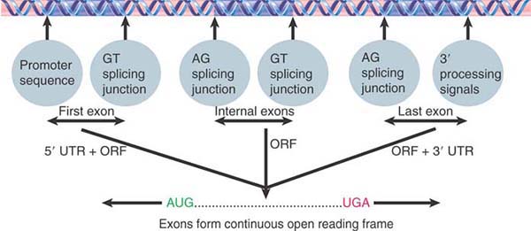
FIGURE 4.3 Exons of protein-coding genes are identified as coding sequences flanked by appropriate signals (with untranslated regions at both ends). The series of exons must generate an ORF with appropriate initiation and termination codons.
The algorithms that are used to connect exons are not completely effective when the gene is very large and the exons might be separated by very large distances. For example, the initial analysis of the human genome mapped 170,000 exons into 32,000 genes. This is incorrect because it gives an average of 5.3 exons per gene, whereas the average of individual genes that have been fully characterized is 10.2. Either we have missed many exons, or they should be connected differently into a smaller number of genes in the entire genome sequence.
Even when the organization of a gene is correctly identified, there is the problem of distinguishing functional genes from pseudogenes. Many pseudogenes can be recognized by obvious defects in the form of multiple mutations that result in nonfunctional coding sequences. Pseudogenes that have originated more recently have not accumulated so many mutations and thus may be more difficult to identify. In an extreme example, the mouse has only one functional encoding glyceraldehyde phosphate dehydrogenase gene (GAPDH), but has about 400 homologous pseudogenes. Approximately 100 of these pseudogenes initially appeared to be functional in the mouse genome sequence, and individual examination was necessary to exclude them from the list of functional genes. Pseudogenes with relatively intact coding sequences but mutated transcription signals are more difficult to identify. (Some pseudogenes encode functional RNAs that play a role in gene regulation; see the Regulatory RNA chapter.)
How can suspected protein-coding genes be verified? If it can be shown that a DNA sequence is transcribed and processed into a translatable mRNA, it is assumed that it is functional. One technique for doing this is reverse transcription polymerase chain reaction (RT-PCR) (see the Methods in Molecular Biology and Genetic Engineering chapter), in which RNA isolated from cells is reverse transcribed to DNA and subsequently amplified to many copies using the polymerase chain reaction. The amplified DNA products can then be sequenced or otherwise analyzed to see if they have the appropriate structural features of a mature transcript.
RT-PCR can also be used for quantitative assessment of gene expression, although there are now better techniques for this purpose. High throughput sequencing of reverse-transcribed RNAs from a cell sample (known as deep RNA sequencing or RNA-seq) allows rapid analysis and quantitation of the sample’s transcriptome. The application of this technique to the genetic model organisms Drosophila and C. elegans has revealed details about gene expression across the genome and the characterization of regulatory networks during development.
Confidence that a gene is functional can be increased by comparing regions of the genomes of different species. There has been extensive overall reorganization of sequences between the mouse and human genomes, as seen in the simple fact that there are 23 chromosomes in the human haploid genome and 20 chromosomes in the mouse haploid genome. However, at the level of individual chromosomal regions, the order of genes is generally the same: When pairs of human and mouse homologs are compared, the genes located on either side also tend to be homologs. This relationship is called synteny.
FIGURE 4.4 shows the relationship between mouse chromosome 1 and the human chromosomal set. Twenty-one segments in this mouse chromosome that have syntenic counterparts in human chromosomes have been identified. The extent of reshuffling that has occurred between the genomes is shown by the fact that the segments are spread among six different human chromosomes. The same types of relationships are found in all mouse chromosomes except for the X chromosome, which is syntenic only with the human X chromosome. This is explained by the fact that the X is a special case, subject to dosage compensation to adjust for the difference between the one copy of males and the two copies of females (see the chapter titled Epigenetics II). This restriction can apply selective pressure against the translocation of genes to and from the X chromosome.
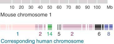
FIGURE 4.4 Mouse chromosome 1 has 21 segments between 1 and 25 Mb in length that are syntenic with regions corresponding to parts of six human chromosomes.
Comparison of the mouse and human genome sequences shows that more than 90% of each genome lies in syntenic blocks that range widely in size from 300 kb to 65 megabases (Mb). There is a total of 342 syntenic segments, with an average length of 7 Mb (0.3% of the genome). Ninety-nine percent of mouse genes have a homolog in the human genome; for 96% that homolog is in a syntenic region.
Comparison of genomes provides interesting information about the evolution of species. The number of gene families in the mouse and human genomes is the same, and a major difference between the species is the differential expansion of particular families in the mouse genome. This is especially noticeable in genes that affect phenotypic features that are unique to the species. Of 25 families for which the size has been expanded in the mouse genome, 14 contain genes specifically involved in rodent reproduction, and 5 contain genes specific to the immune system.
A validation of the importance of the identification of syntenic blocks comes from pairwise comparisons of the genes within them. For example, a gene that is not in a syntenic location (i.e., its context is different in the two species being compared) is twice as likely to be a pseudogene. Put another way, gene translocation away from the original locus tends to be associated with the formation of pseudogenes. Therefore, the lack of a related gene in a syntenic position is grounds for suspecting that an apparent gene might really be a pseudogene. Overall, more than 10% of the genes that are initially identified by analysis of the genome are likely to turn out to be pseudogenes.
As a general rule, comparisons between genomes add significantly to the effectiveness of gene prediction. When sequence features indicating functional genes are conserved—for example, between human and mouse genomes—there is an increased probability that they identify functional orthologs.
Identifying genes encoding RNAs other than mRNA is more difficult because researchers cannot use the criterion of the ORF. It is certainly true that the comparative genome analysis described earlier has increased the rigor of the analysis. For example, analysis of either the human or the mouse genome alone identifies about 500 genes encoding tRNAs, but comparison of their features suggests that fewer than 350 of these genes are in fact functional in each genome.
Researchers can locate a functional gene through the use of an expressed sequence tag (EST), a short portion of a transcribed sequence usually obtained from sequencing one or both ends of a cloned fragment from a cDNA library. An EST can confirm that a suspected gene is actually transcribed or help identify genes that influence particular disorders. Through the use of a physical mapping technique such as in situ hybridization (see the Clusters and Repeats chapter), researchers can determine the chromosomal location of an EST. (In situ hybridization is a technique that identifies the chromosomal location of a specific DNA sequence. We also can use it to determine the number of copies of a sequence in a cell, so it can detect whether there is an abnormal number of a specific chromosome. In this way, it is helpful in identifying cancerous cells, which often have extra copies of some chromosomes. It is also commonly used to diagnose suspected genetic disorders.)
4.6 Some Eukaryotic Organelles Have DNA
The first evidence for the presence of genes outside the nucleus was provided by non-Mendelian inheritance in plants (observed in the early years of the 20th century, just after the rediscovery of Mendelian inheritance). Non-Mendelian inheritance is defined by the failure of the offspring of a mating to display Mendelian segregation for parental characters, therefore indicating the presence of genes that are outside the nucleus and are not distributed to gametes or to daughter cells by segregation on the meiotic or mitotic spindles. FIGURE 4.5 shows that this happens when the mitochondria are inherited from both male and female parents and they have different alleles, so that a daughter cell can receive an unbalanced distribution of mitochondria from only one parent (see the Extrachromosomal Replicons chapter). This is also true of chloroplasts in some plants; both mitochondria and chloroplasts contain genomes with functional genes.

FIGURE 4.5 When mitochondria are inherited from both parents and paternal and maternal mitochondrial alleles differ, a cell has two sets of mitochondrial DNAs. Mitosis usually generates daughter cells with both sets. Somatic variation can result if unequal segregation generates daughter cells with only one set.
The extreme form of non-Mendelian inheritance is uniparental inheritance, which occurs when the genotype of only one parent is inherited and that of the other parent is not passed on to the offspring. In less extreme examples, one parental genotype exceeds the other genotype in the offspring. In animals and most plants, it is the mother whose genotype is preferentially (or solely) inherited. This effect is sometimes described as maternal inheritance. The important point is that the organellar genotype contributed by the parent of one particular sex predominates, as seen in abnormal segregation ratios when a cross is made between mutant and wild type. This contrasts with the expected Mendelian pattern, which occurs when reciprocal crosses show the contributions of both parents to be equally inherited.
Leber’s hereditary optic neuropathy (LHON) is a human disease that shows maternal inheritance. It results from a point mutation in an NADH dehydrogenase subunit gene carried on mitochondrial DNA (mtDNA), a genome that is inherited only maternally, from mothers to both male and female offspring but not from fathers to any children. LHON is characterized by an abrupt loss of vision, usually in both eyes, in young adulthood.
In non-Mendelian inheritance, the bias in parental genotypes is established at, or soon after, the formation of a zygote. There are various possible causes. The contribution of maternal or paternal information to the organelles of the zygote might be unequal; in the most extreme case, only one parent contributes. In other cases, the contributions are equal, but the information provided by one parent does not persist. Combinations of both effects are possible. Whatever the cause, the unequal representation of the information from the two parents contrasts with nuclear genetic information, which derives equally from each parent.
Some non-Mendelian inheritance results from the presence of DNA genomes that are inherited independently of nuclear genes, in mitochondria and chloroplasts. In effect, the organelle genome is a DNA molecule that has been physically sequestered in an isolated part of the cell and is subject to its own form of expression and regulation. An organelle genome can encode some or all of the tRNAs and rRNAs used within that organelle, but encodes only some of the polypeptides needed for normal functioning of the organelle. The other polypeptides are encoded in the nucleus, expressed via the cytoplasmic protein synthetic apparatus, and imported into the organelle.
Genes not residing within the nucleus are generally described as extranuclear genes; they are transcribed and translated in the same organelle compartment (mitochondrion or chloroplast) in which they are carried. By contrast, nuclear genes are expressed by means of cytoplasmic protein synthesis. (The term cytoplasmic inheritance sometimes is used to describe the inheritance of genes in organelles. We will not use this term here because it is important to distinguish between processes in the general cytosol and those in specific organelles.)
Animals show maternal inheritance of mitochondria, which can be explained if the mitochondria are contributed entirely by the ovum and not at all by the sperm. FIGURE 4.6 shows that the sperm contributes only copies of the nuclear chromosomes. Thus the mitochondrial genes are inherited exclusively from the mother, and males do not pass these genes to their offspring. Chloroplasts are generally also maternally inherited, though some plant taxonomic groups (such as some Passiflora [passion flower] species) show paternal or biparental inheritance of chloroplasts.

FIGURE 4.6 In animals, DNA from the sperm enters the oocyte to form the male pronucleus in the fertilized egg, but all the mitochondria are provided by the oocyte.
The chemical environment of organelles is different from that of the nucleus; therefore, organelle DNA evolves at its own distinct rate. If inheritance is uniparental, there can be no recombination between parental genomes. In fact, recombination usually does not occur in those cases in which organelle genomes are inherited from both parents. Organelle DNA has a different replication system from that of the nucleus; as a result, the error rate during replication might be different. Mitochondrial DNA accumulates mutations more rapidly than nuclear DNA in mammals, but in plants the accumulation of mutations in the mitochondrial DNA is slower than in nuclear DNA; chloroplast DNA has an intermediate mutation rate.
One consequence of maternal inheritance is that the sequence variation in mitochondrial DNA is more sensitive than nuclear DNA to reductions in the size of the breeding population. Comparisons of mitochondrial DNA sequences in a range of human populations allow a phylogenetic “tree,” showing the branching lineages of mitochondrial DNA variants over time, to be constructed. The divergence among human mitochondrial DNAs spans 0.57%. A tree can be constructed in which the mitochondrial variants diverged from a common (African) ancestor. The rate at which mammalian mitochondrial DNA accumulates mutations is 2% to 4% per million years, which is more than 10 times faster than the rate for (nuclear) globin gene substitutions. Such a rate would generate the observed divergence over an evolutionary period of 140,000 to 280,000 years. This implies that human mitochondrial DNA is descended from a single population that lived in Africa approximately 200,000 years ago. This cannot be interpreted as evidence that there was only a single population at that time, however; there might have been many populations, and some or all of them might have contributed to modern human nuclear genetic variation.
4.7 Organelle Genomes Are Circular DNAs That Encode Organelle Proteins
Most organelle genomes take the form of a single circular molecule of DNA of unique sequence (denoted mtDNA in the mitochondrion and ctDNA or cpDNA in the chloroplast). There are a few exceptions in unicellular eukaryotes for which mitochondrial DNA is a linear molecule.
Usually there are several copies of the genome in the individual organelle. There are multiple organelles per cell; therefore, there are many organelle genomes per cell, so the organelle genome can be considered a repetitive sequence.
Chloroplast genomes are relatively large, usually about 140 kb in higher plants and less than 200 kb in unicellular eukaryotes. This is comparable to the size of a large bacteriophage genome, such as that of T4 at about 165 kb. There are multiple copies of the genome per organelle, typically 20 to 40 in a higher plant, and multiple copies of the organelle per cell, typically 20 to 40.
Mitochondrial genomes vary in total size by more than an order of magnitude. Animal cells have small mitochondrial genomes (approximately 16.6 kb in mammals). There are several hundred mitochondria per cell and each mitochondrion has multiple copies of the DNA. The total amount of mitochondrial DNA relative to nuclear DNA is small; it is estimated to be less than 1%.
In yeast, the mitochondrial genome is much larger. In Saccharomyces cerevisiae, the exact size varies among different strains but averages about 80 kb. There are about 22 mitochondria per cell, which corresponds to about 4 genomes per organelle. In dividing cells, the proportion of mitochondrial DNA can be as high as 18%. See TABLE 4.1 and FIGURE 4.7 for information about the content of the mitochondrial genome and a map of the human mitochondrial genome.

FIGURE 4.7 Human mitochondrial DNA has 22 tRNA genes, 2 rRNA genes, and 13 protein-coding regions. Fourteen of the 15 protein-coding and rRNA-coding regions are transcribed in the same direction. Fourteen of the tRNA genes are expressed in the clockwise direction and 8 are read counterclockwise.
TABLE 4.1 Mitochondrial genomes have genes encoding (mostly complex I–IV) proteins, rRNAs, and tRNAs.
| Species | Size (kb) | Protein-Coding Genes | RNA-Coding Genes |
|---|---|---|---|
| Fungi | 19–100 | 8–14 | 10–28 |
| Protists | 6–100 | 3–62 | 2–29 |
| Plants | 186–366 | 27–34 | 21–30 |
| Animals | 16–17 | 13 | 4–24 |
Plants show an extremely wide range of variation in mitochondrial DNA size, with a minimum size of about 100 kb. The size of the genome makes it difficult to isolate, but restriction mapping in several plants suggests that the mitochondrial genome is usually a single sequence that is organized as a circle. Within this circle there are multiple copies of short homologous sequences. Recombination between these elements generates smaller, subgenomic circular molecules that coexist with the complete “master” genome—a good example of the apparent complexity of plant mitochondrial DNAs.
With mitochondrial genomes sequenced from many organisms, we can now see some general patterns in the representation of functions in mitochondrial DNA. Table 4.1 summarizes the distribution of genes in mitochondrial genomes. The total number of protein-coding genes is rather small and does not correlate with the size of the genome. The 16.6-kb mammalian mitochondrial genomes encode 13 proteins, whereas the 60- to 80-kb yeast mitochondrial genomes encode as few as 8 proteins. The much larger plant mitochondrial genomes encode more proteins. Introns are found in most mitochondrial genes, although not in the very small mammalian genomes.
The two major rRNAs are always encoded by the mitochondrial genome. The number of tRNAs encoded by the mitochondrial genome varies from none to the full complement (25 to 26 in mitochondria). This accounts for the variation in Table 4.1.
The major part of the protein-coding activity is devoted to the components of the multisubunit assemblies of respiration complexes I–IV. Many ribosomal proteins are encoded in protist and plant mitochondrial genomes, but there are few or none in fungi and animal genomes. There are genes encoding proteins involved in cytoplasm-to-mitochondrion import in many protist mitochondrial genomes.
Animal mitochondrial DNA is extremely compact. There are extensive differences in the detailed gene organization found in different animal taxonomic groups, but the general principle of a small genome encoding a restricted number of functions is maintained. In mammalian mitochondria, the genome is particularly compact. There are no introns, some genes actually overlap, and almost every base pair can be assigned to a gene. With the exception of the D-loop, a region involved with the initiation of DNA replication, no more than 87 of the 16,569 bp of the human mitochondrial genome lie in intergenic regions.
The complete nucleotide sequences of animal mitochondrial genomes show extensive homology in organization. The map of the human mitochondrial genome is shown in Figure 4.7. There are 13 protein-coding regions. All of the proteins are components of the electron transfer system of cellular respiration. These include cytochrome b, three subunits of cytochrome oxidase, one of the subunits of ATPase, and seven subunits (or associated proteins) of NADH dehydrogenase.
The fivefold discrepancy in size between the S. cerevisiae (84 kb) and mammalian (16.6 kb) mitochondrial genomes alone alerts us to the fact that there must be a great difference in their genetic organization in spite of their common function. The number of endogenously synthesized products concerned with mitochondrial enzymatic functions appears to be similar. Does the additional genetic material in yeast mitochondria encode other proteins, perhaps concerned with regulation, or is it unexpressed?
The map in FIGURE 4.8 accounts for the major RNA and protein products of the yeast mitochondrion. The most notable feature is the dispersion of loci on the map.
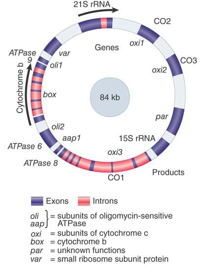
FIGURE 4.8 The mitochondrial genome of S. cerevisiae contains both interrupted and uninterrupted protein-coding genes, rRNA genes, and tRNA genes (positions not indicated). Arrows indicate direction of transcription.
The two largest loci are the interrupted genes box (encoding cytochrome b) and oxi3 (encoding subunit 1 of cytochrome oxidase). Together these two genes are almost as long as the entire mitochondrial genome in mammals! Many of the long introns in these genes have ORFs in register with the preceding exon (see the Catalytic RNA chapter). This adds several proteins, all synthesized in low amounts, to the complement of the yeast mitochondrion.
The remaining genes are uninterrupted. They correspond to the other two subunits of cytochrome oxidase encoded by the mitochondrion, to the subunit(s) of the ATPase, and (in the case of var1) to a mitochondrial ribosomal protein. The total number of yeast mitochondrial protein-coding genes is unlikely to exceed about 25.
4.8 The Chloroplast Genome Encodes Many Proteins and RNAs
What genes are carried by chloroplasts? Chloroplast DNAs vary in length from about 120 to 217 kb (the largest in geranium). The sequenced chloroplast genomes (more than 200 in total) have 87 to 183 genes. TABLE 4.2 summarizes the functions encoded by the chloroplast genome in land plants. There is more variation in the chloroplast genomes of algae.
TABLE 4.2 The chloroplast genome in land plants encodes 4 rRNAs, 30 tRNAs, and about 60 proteins.
| Genes | Types |
|---|---|
| RNA coding | |
| 16S rRNA | 1 |
| 23S rRNA | 1 |
| 4.5S rRNA | 1 |
| 5S rRNA | 1 |
| tRNA | 30–32 |
| Gene expression | |
| Proteins | 20–21 |
| RNA polymerase | 3 |
| Others | 2 |
| Chloroplast functions | |
| Rubisco and thylakoids | 31–32 |
| NADH dehydrogenase | 11 |
| Total | 105–113 |
The chloroplast genome is generally similar to that of mitochondria, except that there are more genes. The chloroplast genome encodes all the rRNAs and tRNAs needed for protein synthesis in the chloroplast. The ribosome includes two small rRNAs in addition to the major ones. The tRNA set can include all of the necessary genes. The chloroplast genome encodes about 50 proteins, including RNA polymerase and ribosomal proteins. Again, the rule is that organelle genes are transcribed and translated within the organelle. About half of the chloroplast genes encode proteins involved in protein synthesis.
Introns in chloroplasts fall into two general classes. Those in tRNA genes are usually (although not inevitably) located in the anticodon loop, like the introns found in yeast nuclear tRNA genes (see the RNA Splicing and Processing chapter). Those in protein-coding genes resemble the introns of mitochondrial genes (see the Catalytic RNA chapter). This places the endosymbiotic event at a time in evolution before the separation of prokaryotes with uninterrupted genes.
The chloroplast is the site of photosynthesis. Many of its genes encode proteins of photosynthetic complexes located in the thylakoid membranes. The constitution of these complexes shows a different balance from that of mitochondrial complexes. Although some complexes are like mitochondrial complexes in that they have some subunits encoded by the organelle genome and some by the nuclear genome, other chloroplast complexes are encoded entirely by one genome. For example, the gene for the large subunit of ribulose bisphosphate carboxylase (RuBisCO, which catalyzes the carbon fixation reaction of the Calvin cycle), rbcL, is contained in the chloroplast genome; variation in this gene is frequently used as a basis for reconstructing plant phylogenies. However, the gene for the small RuBisCO subunit, rbcS, is usually carried in the nuclear genome. On the other hand, genes for photosystem protein complexes are found on the chloroplast genome, whereas those for the light-harvesting complex (LHC) proteins are nuclear encoded.
4.9 Mitochondria and Chloroplasts Evolved by Endosymbiosis
How is it that an organelle evolved so that it contains genetic information for some of its functions, whereas the information for other functions is encoded in the nucleus? FIGURE 4.9 shows the endosymbiotic hypothesis for mitochondrial evolution, in which primitive cells captured bacteria that provided the function of cellular respiration and over time evolved into mitochondria. At first, the proto-organelle must have contained all of the genes needed to specify its functions. A similar mechanism has been proposed for the origin of chloroplasts.
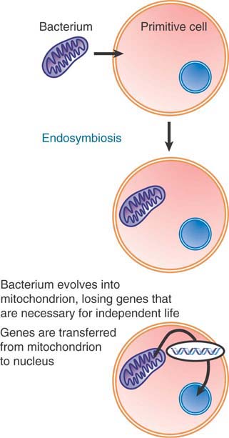
FIGURE 4.9 Mitochondria originated by an endosymbiotic event when a bacterium was captured by a eukaryotic cell.
Sequence homologies suggest that mitochondria and chloroplasts evolved separately from lineages that are common with different eubacteria, with mitochondria sharing an origin with α-purple bacteria and chloroplasts sharing an origin with cyanobacteria. The closest known relative of mitochondria among the bacteria is Rickettsia (the causative agent of typhus, Rocky Mountain spotted fever, and several other infectious diseases carried by arthropod vectors), which is an obligate intracellular parasite that is probably descended from free-living bacteria. This reinforces the idea that mitochondria originated in an endosymbiotic event involving an ancestor that is also common to Rickettsia.
The endosymbiotic origin of the chloroplast is emphasized by the relationships between its genes and their counterparts in bacteria. The organization of the rRNA genes in particular is closely related to that of a cyanobacterium, which pins down more precisely the last common ancestor between chloroplasts and bacteria. Not surprisingly, cyanobacteria are photosynthetic.
At least two changes must have occurred as the bacterium became integrated into the recipient cell and evolved into the mitochondrion (or chloroplast). The organelles have far fewer genes than an independent bacterium and have lost many of the gene functions that are necessary for independent life (such as metabolic pathways). The majority of genes encoding organelle functions are in fact now located in the nucleus, so these genes must have been transferred there from the organelle.
Transfer of DNA between an organelle and the nucleus has occurred over evolutionary history and still continues. The rate of transfer can be measured directly by introducing a gene that can function only in the nucleus (because it contains a nuclear intron, or because the protein must function in the cytosol) into an organelle. In terms of providing the material for evolution, the transfer rates from organelle to nucleus are roughly equivalent to the rate of single gene mutation. DNA introduced into mitochondria is transferred to the nucleus at a rate of 2 × 10⁻⁵ per generation. Experiments to measure transfer in the reverse direction, from nucleus to mitochondrion, suggest that the rate is much lower, less than 10−10. When a nuclear-specific antibiotic resistance gene is introduced into chloroplasts, its transfer to the nucleus and successful expression can be detected by screening seedlings for resistance to the antibiotic. This shows that transfer occurs at a rate of 1 in 16,000 seedlings, or 6 × 10⁻⁵ per generation.
Transfer of a gene from an organelle to the nucleus requires physical movement of the DNA, of course, but successful expression also requires changes in the coding sequence. Organelle proteins that are encoded by nuclear genes have special sequences that allow them to be imported into the organelle after they have been synthesized in the cytoplasm. These sequences are not required by proteins that are synthesized within the organelle. Perhaps the process of effective gene transfer occurred at a period when compartments were less rigidly defined, so that it was easier both for the DNA to be relocated and for the proteins to be incorporated into the organelle regardless of the site of synthesis.
Phylogenetic analyses show that gene transfers have occurred independently in many different lineages. It appears that transfers of mitochondrial genes to the nucleus occurred only early in animal cell evolution, but it is possible that the process is still continuing in plant cells. The number of transfers can be large; there are more than 800 nuclear genes in Arabidopsis, whose sequences are related to genes in the chloroplasts of other plants. These genes are candidates for evolution from genes that originated in the chloroplast.
Summary
The DNA sequences composing a eukaryotic genome can be classified into three groups:
Nonrepetitive sequences that are unique
Moderately repetitive sequences that are dispersed and repeated a small number of times, with some copies not being identical
Highly repetitive sequences that are short and usually repeated as tandem arrays
The proportions of these types of sequences are characteristic for each genome, although larger genomes tend to have a smaller proportion of nonrepetitive DNA. Almost 50% of the human genome consists of repetitive sequences, the majority corresponding to transposon sequences. Most structural genes are located in nonrepetitive DNA. The amount of nonrepetitive DNA is a better reflection of the complexity of the organism than the total genome size; the greatest amount of nonrepetitive DNA in genomes is about 2 × 10⁹ bp.
Non-Mendelian inheritance is explained by the presence of DNA in organelles in the cytoplasm. Mitochondria and chloroplasts are membrane-bound systems in which some proteins are synthesized within the organelle, whereas others are imported. The organelle genome is usually a circular DNA that encodes all the RNAs and some of the proteins required by the organelle.
Mitochondrial genomes vary greatly in size, from the small 16.6-kb mammalian genome to the 570-kb genome of higher plants. The larger genomes might encode additional functions. Chloroplast genomes range in size from about 120 to 217 kb. Those that have been sequenced have similar organizations and coding functions. In both mitochondria and chloroplasts, many of the major proteins contain some subunits synthesized in the organelle and some subunits imported from the cytosol. Transfers of DNA have occurred between chloroplasts or mitochondria and nuclear genomes.
References
4.2 Genome Mapping Reveals That Individual Genomes Show Extensive Variation
Review
Levy, S., and Strausberg, R. L. (2008). Human genetics: individual genomes diversify. Nature 456, 49–51.
Research
The 1000 Genomes Project Consortium. (2015). A global reference for human genetic variation. Nature 526, 68–74.
Altshuler, D., et al. (2005). A haplotype map of the human genome. Nature 437, 1299–1320.
Altshuler, D., et al. (2000). An SNP map of the human genome generated by reduced representation shotgun sequencing. Nature 407, 513–516.
Mullikin, J. C, et al. (2000). An SNP map of human chromosome 22. Nature 407, 516–520.
Sudmant, P. H., and 82 others. (2015). An integrated map of structural variation in 2,504 human genomes. Nature 526, 75–81.
4.3 SNPs Can Be Associated with Genetic Disorders
Reviews
Bush, W. S., and Moore, J. H. (2012). Genome-wide association studies. PLoS. Comput. Biol. 8, e1002822.
Gusella, J. F. (1986). DNA polymorphism and human disease. Annu. Rev. Biochem. 55, 831–854.
Research
Altshuler, D., et al. (2005). A haplotype map of the human genome. Nature 437, 1299–1320.
Dib, C., et al. (1996). A comprehensive genetic map of the human genome based on 5,264 microsatellites. Nature 380, 152–154.
Dietrich, W. F., et al. (1996). A comprehensive genetic map of the mouse genome. Nature 380, 149–152.
Hinds, D. A., et al. (2005). Whole-genome patterns of common DNA variation in three human populations. Science 307, 1072–1079.
Sachidanandam, R., et al. (2001). A map of human genome sequence variation containing 1.42 million single nucleotide polymorphisms. The International SNP Map Working Group. Nature 409, 928–933.
4.4 Eukaryotic Genomes Contain Nonrepetitive and Repetitive DNA Sequences
Reviews
Britten, R. J., and Davidson, E. H. (1971). Repetitive and nonrepetitive DNA sequences and a speculation on the origins of evolutionary novelty. Q. Rev. Biol. 46, 111–133.
Davidson, E. H., and Britten, R. J. (1973). Organization, transcription, and regulation in the animal genome. Q. Rev. Biol. 48, 565–613.
4.5 Eukaryotic Protein-Coding Genes Can Be Identified by the Conservation of Exons and of Genome Organization
Research
Buckler, A. J., et al. (1991). Exon amplification: a strategy to isolate mammalian genes based on RNA splicing. Proc. Natl. Acad. Sci. USA 88, 4005–4009.
Gerstein, M. B., et al. (2010). Integrative analysis of the Caenorhabditis elegans genome by the modENCODE Project. Science 330, 1775–1787.
Kunkel, L. M., et al. (1985). Specific cloning of DNA fragments absent from the DNA of a male patient with an X chromosome deletion. Proc. Natl. Acad. Sci. USA 82, 4778–4782.
Monaco, A. P., et al. (1985). Detection of deletions spanning the Duchenne muscular dystrophy locus using a tightly linked DNA segment. Nature 316, 842–845.
Su, A. I., et al. (2004). A gene atlas of the mouse and human protein-encoding transcriptome. Proc. Natl. Acad. Sci. USA 101, 6062–6067.
The modENCODE Consortium, et al. (2010). Identification of functional elements and regulatory circuits by Drosophila modENCODE. Science 330, 1787–1797.
4.6 Some Eukaryotic Organelles Have DNA
Research
Cann, R. L., et al. (1987). Mitochondrial DNA and human evolution. Nature 325, 31–36.
4.7 Organelle Genomes Are Circular DNAs That Encode Organelle Proteins
Reviews
Attardi, G. (1985). Animal mitochondrial DNA: an extreme example of economy. Int. Rev. Cytol. 93, 93–146.
Boore, J. L. (1999). Animal mitochondrial genomes. Nucleic. Acids. Res. 27, 1767–1780.
Clayton, D. A. (1984). Transcription of the mammalian mitochondrial genome. Annu. Rev. Biochem. 53, 573–594.
Gray, M. W. (1989). Origin and evolution of mitochondrial DNA. Annu. Rev. Cell Biol. 5, 25–50.
Lang, B. F., et al. (1999). Mitochondrial genome evolution and the origin of eukaryotes. Annu. Rev. Genet. 33, 351–397.
Research
Anderson, S., Bankier, A. T., Barrell, B. G., et al. (1981). Sequence and organization of the human mitochondrial genome. Nature 290, 457–465.
4.8 The Chloroplast Genome Encodes Many Proteins and RNAs
Reviews
Palmer, J. D. (1985). Comparative organization of chloroplast genomes. Annu. Rev. Genet. 19, 325–354.
Shimada, H., and Sugiura, M. (1991). Fine structural features of the chloroplast genome: comparison of the sequenced chloroplast genomes. Nucleic. Acids. Res. 11, 983–995.
Sugiura, M., et al. (1998). Evolution and mechanism of translation in chloroplasts. Annu. Rev. Genet. 32, 437–459.
4.9 Mitochondria and Chloroplasts Evolved by Endosymbiosis
Review
Lang, B. F., et al. (1999). Mitochondrial genome evolution and the origin of eukaryotes. Annu. Rev. Genet. 33, 351–397.
Research
Adams, K. L., et al. (2000). Repeated, recent and diverse transfers of a mitochondrial gene to the nucleus in flowering plants. Nature 408, 354–357.
Arabidopsis Initiative (2000). Analysis of the genome sequence of the flowering plant Arabidopsis thaliana. Nature 408, 796–815.
Huang, C. Y., et al. (2003). Direct measurement of the transfer rate of chloroplast DNA into the nucleus. Nature 422, 72–76.
Thorsness, P. E., and Fox, T. D. (1990). Escape of DNA from mitochondria to the nucleus in S. cerevisiae. Nature 346,376–379.