After completing this chapter, you should be able to
• Define a hard disk drive, describe the various types of hard disk interfaces, and list the components of a hard disk
• Explain solid-state drives, CD-ROM/DVD file systems, RAID storage systems, and RAID levels
• Describe disk partitions and provide an overview of the physical and logical structures of a hard disk
• Describe file systems; explain the various types of file systems; provide an overview of Windows, Linux, Mac OS X, and Solaris 10 file systems; and explain file system analysis using the Sleuth Kit
• Explain how to recover deleted partitions and deleted files in Windows, Mac, and Linux, as well as how to identify the creation date, last accessed date of a file, and deleted subdirectories
• List partition recovery tools and file recovery tools for Windows, Mac OS X, and Linux
• Summarize steganography and its types, list the various applications of steganography, and discuss various digital steganography techniques
• Define steganalysis and explain how to detect steganography
• List various steganography detection tools and picture viewer and graphics file forensic tools, describe how to compress data, and describe how to process forensic images using MATLAB
• Explain Windows and Mac OS X boot processes
Now that we have created a forensically sound copy of a device’s persistent storage, it’s time to begin our forensic analysis of that data. We are still in the extraction phase, however, in that we are still in the process of extracting evidence from the raw materials we’ve collected. We won’t start our actual analysis until we’ve extracted all the binary objects that will provide information that help us determine which of these digital objects has evidentiary value.
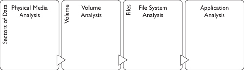
Brian Carrier, in his book File System Forensic Analysis details a path from the physical medium all the way through application analysis, as detailed in Figure 6-1.1 Our discussion of persistent storage parallels this model and helps make sense out of the seemingly random stream of bits that we have in our forensic copy.
Figure 6-1 Levels of abstraction in disk analysis (Adapted from Carrier, B. File System Forensic Analysis (NJ: Pearson, 2005), p. 10.)
As a digital forensics investigator (DFI), you need to understand how persistent storage is organized. While it would be convenient to focus just on files and file systems, you need to understand the physical layout of the disk drive in order to understand how data can be hidden on the disk so that it’s not accessible via a file system interface.

NOTE Since I’m sure you’re wondering, “spinning rust” is a nickname for disk drives, based on the color of the individual disk platters.
At this time, there are two kinds of disk drives available: the regular kind of hard disk drives (HDD) and the new solid-state drives (SSDs). You may still find the plastic-covered 3¼” drives (diskettes) shown in Figure 6-2, and you need to have a drive capable of reading those disks.

Figure 6-2 3.5”, 2/5”, 3¼” floppy drive, and USB stick
Reading these disks may require an external driver (mine has a universal serial bus [USB] interface), since most computers manufactured in the last five years or so haven’t included a so-called floppy drive (it’s been replaced by an optical drive, or in some cases, an optical drive and a floppy drive that can be switched in and out). The original 8” floppy disks (and they were floppy—you could bend them in half), as well as the 5.5” floppies, are even rarer birds.

TIP You may not need to own an 8.5” floppy drive or a 3.5” drive, but it’s prudent to do enough research to know where to find one in a hurry.
When we think of nonvolatile storage, our first thought is hard disk drives (HDDs). These hard disk drives are usually complex compared to floppy disks. These days, the most common sizes of hard disks are the 2.5-inch form factor for notebooks and laptops, and a 3.5-inch form factor for larger PCs. Inside a PC, if there are two disks and the interface is integrated drive electronics (IDE) or parallel advanced technology attachment (PATA), then one of the disks is designated as the primary and one is secondary, although you may hear them referred to as master and slave. (As an aside, the original spec never mentions master and slave. The devices are referred to as device0 and device1.) The terms device0 and device1 aren’t used with current serial advanced technology attachment (SATA) drives.
A hard disk drive is a form of nonvolatile storage that uses magnetic media and can maintain data even in the absence of electricity. Another term for this is persistent storage. While the original definition of a hard disk was useful to compare and distinguish it from other forms of digital media (magnetic tape, floppy disks), nowadays, defining a hard disk is based on a particular interface specification and the protocols to which the storage medium responds. We’ll learn later in this chapter that a solid-state drive (SSD) supports a standard interface and can be treated as if it was a hard disk drive, even though the technology used is vastly different from the earlier technologies.
First, a hard disk consists of a spindle, upon which are stacked disk platters. Data are stored on those platters in concentric circles called tracks, and each track consists of some number of disk sectors (usually 512 bytes per sector). Read/write heads, driven by an actuator motor, can move across the surfaces of the platters to read from each track. Each prescribed stopping place for the read/write heads is called a cylinder. Figure 6-3 shows the different parts of an HDD.2
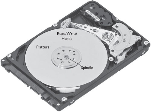
Figure 6-3 Disk drive internals
There are 1,024 tracks per platter, numbered from 0 (the outermost track on the platter) to 1,023 (the innermost track on the platter), and a given number of sectors per track. Computing the total capacity of a drive is a function of the number of tracks, sectors per track, bytes per sector, and the number of read/write heads supported by the device. The resulting formula looks like this:
Total disk capacity = (bytes/sector) * (sectors/track) * (tracks/surface) * # of surfaces
We can simplify that formula to be
Total disk capacity = (bytes/sector) * (sectors/track) * (total tracks)
One 2.5” drive I have lists the following specifications: 13,424 cylinders, 15 heads, 63 sectors/track. Calculating the capacity is 512 * 63 * 13424 * 15 = 6.49 gigabytes (GB), which fortunately corresponds to the amount stated on the drive.
The computer identifies the location of the desired sector by using a sector address. The earliest form of addressing was CHS (cylinder, head, and sector). The address of the first sector on the disk would be (0, 0, 1). The first sector on the second header would be (0, 1, 1). CHS turned out to be unwieldy to use, as well as limiting the size of the disk that could be addressed, and was replaced by Logical Block Addressing (LBA). Here, the first sector of the disk is numbered 0, which is the same as CHS (0, 0, 1). LBA 2 is CHS (0, 0, 2).
One more thing: Although the size of a disk sector is usually fixed by the manufacturer, formatting the disk will allow you to specify the file system block size. The file system block size is a multiple of the sector size: 1,024, 4,028, and higher are common sizes. These file system blocks are also referred to as clusters (another overused word). The key point here is that the cluster size determines how much disk space is allocated to a single file. If the cluster size is 1,024 and the file size is 24, there are 1,000 bytes unused; this unused space is referred to as slack space. Slack space isn’t the same as unallocated space, which refers to clusters that aren’t assigned to any file (sometimes referred to as being on the “free list”). Unallocated space also isn’t the same as clusters that are marked as associated with a file but no such file exists. These clusters are called orphans or lost clusters because they are unavailable to the operating system (OS) for allocation to another file… indeed, a waste of space.
The OS uses a particular protocol to send commands to the disk controller that manages read/write activity as well as using seek() commands to position the read/write heads. Communicating from the OS to the disk controller, as well as transferring data, depends on the physical interface of the device. Common interface types are
• ATA (PATA), SATA
• IDE, EIDE
• Fibre Channel (F-C)
• SCSI (small computer system interface)
Hard disks attach to the computer using a particular kind of interface. ATA stood for advanced technology attachment, and came to be called PATA (parallel ATA). SATA (serial ATA) cut down the number of pins needed in the attachment cable, as well as increasing the speed of the interface. SATA appeared in the ATA-7 specification that was released in 2003: The latest version is ATAPI-8, draft 2, released in 2006.
IDE is an acronym for integrated drive electronics, and EIDE is an acronym for enhanced IDE. Both of these interfaces actually use the ATA specification, but IDE indicated that the device controller was actually built into the drive’s logic board. IDE corresponded to ATA-1, while EIDE contained some capabilities that were defined in the soon-to-be-published ATA-2 standard.
USB is short for Universal Serial Bus. It supports many different peripherals, including keyboards, mice, digital cameras, and digital audio devices. With the help of a USB hub, up to 227 devices can be connected to a single computer at one time. USB also provides an interface for hard disks that can be mounted in cases that provide a USB connection and that plugs into a USB port on the computer. The current standard for USB is 2.0, but it is backward compatible with the earlier 1.0 and 1.1 standards. USB 3.0 has appeared recently and promises to become the new standard for USB drives.
SCSI stands for small computer system interface, and provides faster transfer than IDE/EIDE. You can add a SCSI disk by adding a SCSI controller card and an expansion slot onto a computer. SCSI daisy-chains the disks together and allows for 16 disks (numbered 0 through 15).
Last, Fibre Channel is yet another American National Standards Institute (ANSI) standard that uses optical fiber to connect a device to storage devices. You won’t usually encounter Fibre Channel interfaces outside of a data center. Fibre Channel technology once was the workhorse of storage area networks (SANs), although these days you may find SANs using iSCSI interfaces (SCSI over IP) as well as Fibre Channel over IP (FCIP). Gigabit Ethernet has come to challenge Fibre Channel as the medium of choice within data centers, primarily because of cost.
NOTE It’s the SCSI protocol that actually provides the commands to the disk controller; Fibre Channel and IP are the network protocols that send it on its way.
The physical structure of an HDD consists of sectors, tracks, and cylinders. Although a DFI needs to understand these structures and may find it necessary to work at that level using appropriate tools, higher-level abstractions make the problem of working with disk drives more tractable.
The Host-Protected Area and the Device Configuration Overlay
Before we leave the subject of the physical structure of a hard disk, there are two areas on an HDD that aren’t usually accessible by ordinary user commands. These are the host-protected area (HPA), introduced in ATA-4, and the device configuration overlay (DCO), introduced in ATA-6. The intent of the HPA was to create a space on the disk where a vendor could locate information that wouldn’t be overwritten if the device were physically formatted. The intent of the DCO was to allow configuration changes that would limit the capabilities of the disk in some ways, such as showing a smaller size or indicating that certain features were unimplemented. The DCO can hide sectors allocated to itself and to the HPA, if one exists. On a 40GB hard disk with a 1-GB DCO and a 1-GB HPA, the DCO would show the size of the disk to be 38GB. The reason a DFI needs to know this is that these areas can contain hidden data, executable files, or both. However, this requires that the suspect has access to tools that can actually access these areas on the disk and that the suspect has appropriate permissions to do so.
Partitions A partition is logical structure overlaid on a physical HDD, and is represented as a series of entries in a table that indicate a starting block and a length. Following Brian Carrier,3 I’m going to make the distinction between partitions and volumes. A partition has all its sectors on one physical disk, whereas a volume may have sectors on multiple physical disks. Unless it’s necessary, I’ll follow the convention of using the word “partition” to indicate a volume on a single physical disk and the word “volume” to indicate a volume defined across multiple physical drives.

EXAM TIP A partition will refer to a single volume unless specified otherwise.
Figure 6-4 shows the format of an MS-DOS partition table that is contained in the master boot record (MBR) of a disk specified as a boot disk. The first two entries are primary partitions (as opposed to extended), one labeled as a recovery partition and one labeled as the primary partition that contains the OS. Partition 0 is an extended partition that covers the rest of the disk and contains two logical partitions.
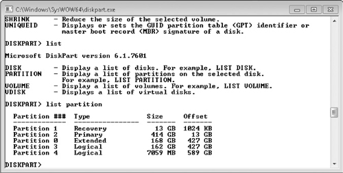
Figure 6-4 Diskpart display of partitions on disk 0
Figure 6-5 shows the same information but in a much friendlier format. Right-clicking the icon in the topmost window brings up a menu that, among other things, will allow you to delete that particular volume.

Figure 6-5 Disk Management window
Notice that the graphic in the lower portion of the screen doesn’t indicate the extended partition; rather, we only see the two logical partitions, both marked as primary.
We’ve mentioned USB drives previously based on their hardware connection to a digital device. Both USB drives and SSDs differ markedly from the technologies that we’re used to in the HDD world. Both of these device types use flash memory chips instead of magnetic surfaces to record data. Both require memory chips that don’t lose data when disconnected from a power supply.
Flash Memory Cards The cards, or “sticks,” come in form factors, such as SD and microSD, with storage from 2GB all the way up to 64GB and more. All of these devices require a card reader of the appropriate type to actually read the contents of the card. Common uses of these cards include removable storage for cameras or handheld devices (old-school personal digital assistants [PDAs] and now smart phones, tablet computers, and netbooks).
USB Drives Like flash memory cards, USB (Universal Serial Bus) drives (sometimes called pen drives since they are small enough to be installed in the head of a ballpoint pen) use flash memory for storage, but they also contain a controller such that they can be plugged directly into a USB connector on a digital device. Capacity varies from 64MB to 64GB and more.
Both flash memory cards and USB drives usually have a physical switch that puts the device into read-only mode, which is useful for acquiring data from the drive. USB drives can also be configured as boot devices; I personally have an 8GB drive that loads the Samurai Web Testing Framework from InGuardians. Larger bootable drives (4GB+) allow the OS to save configuration information on local storage between uses.
Another use for USB drives is for portable software—software that is packaged to run from the USB drive and save all configuration and personal data to that USB drive. This differs from the previously mentioned use of a USB drive because the drive requires an OS to actually run the files (the software from www.portableapps.com requires a Windows OS). If a suspect has been using this kind of device, certain log and history files may be stored on the USB drive and not on the HDD of the desktop or laptop computer.
SSD Drives The advent of solid-state drives (SSDs) has caused some consternation within the forensics community due to the way that data are managed on the SSD drive. Because of issues of wear (NAND memory can only be written to approximately 100,000 times), the drive controller will move a logical disk block from memory block to memory block as a way of wear-leveling access to each memory block. The sequential nature of block allocation on HDD doesn’t apply to SSD drives.
Two issues further complicate retrieving data. Many manufacturers provide a SECURE ERASE function that will either automatically erase the entire drive or, in the case of encrypted driver, delete the encryption key. A second issue is how memory blocks are freed (marked as reusable). In order to inform the controller that a block marked as “Not In Use” is ready to be reused, applications can ask the controller to TRIM these blocks, with the result that these blocks are placed on a queue for the garbage collection (GC) process to erase (overwritten with all 1’s) and marked as free.
All of this depends on whether the OS in question actually supports the TRIM command. Some older SSDs do not support this command, and the TRIM command is only fully supported for NT File System (NTFS) partitions and not for File Allocation Table (FAT) partitions.4
CD-ROM (Compact Disc Read-Only Memory) (usually abbreviated to CD) and DVD (Digital Video Disc) are different specifications for optical drives. CDs are capable of storing about 700MB, while a DVD can store up to 4GBs (8GBs if recorded double-sided). CD/DVD media are usually formatted according to the ISO 9660 standard. Common extensions to that standard are Rock Ridge, which supports long filenames (128 characters) for Unix; Joliet extensions, which support 64-character filenames for Windows; and the El Torito extensions, which allow a CD/DVD to be used as a boot device.
We mentioned earlier that one of the things to avoid when transporting or storing digital devices was electromagnetic radiation (such as speakers). Fortunately, we don’t have to be concerned with that for CD or DVDS, since they are electro-optical media and aren’t affected by electromagnetic radiation. But since they are not encased when in use, they can be altered by scratches, especially scratches that follow the single data track that begins at the center of the platter and grows outward to the outside edge of the disk.
Blu-ray is a more recent recording technique for optical media that utilizes a blue laser instead of a red laser. Blue lasers can be focused more precisely, which allows for increased packing density. Blu-ray discs can store anywhere from 25GB (single layer) to 50GB (dual layer). In order to support the increased density, Blu-ray relies on newer hard-coating technologies to prevent scratches. Combined with improved error-correction algorithms, this means that Blu-ray disks are increasingly resistant to damage from scratches.
RAID originally stood for “redundant array of inexpensive disks,” although the acronym is usually expanded nowadays as “redundant array of independent disks,” perhaps because of the expense of several commercial RAID systems. The idea behind it is strikingly simple: Instead of buying ever-increasing capacity on single drives, spread the storage load across multiple drives, which appear to the host OS as a single volume. RAID uses three strategies to achieve its goal:
• Mirroring, in which a write to a disk block on one drive is copied (mirrored) to a disk block on a second drive.
• Striping, where a byte or a block is written across multiple drives in stripes.
• Parity, where parity blocks are replicated across multiple drives. Parity is defined as a value that is computed such that the value of one of the elements that make up the calculations can be lost, but it’s possible to recompute that value based on the parity settings.
Here’s an example of how parity works. Imagine we have three values: A is 1, B is 0, and C is 0. We use the binary operation XOR (exclusive OR) to compute the parity. A xor B is 1 and 1 xor C is 1, so the parity calculation for these values is 1. If we lost C, we still have A and B. A xor B is 1, and parity is 1. Given how the xor function works, we know that C must have the value 0 if the parity is set to 1.
NOTE xor is defined as 1 if A is 1 or B is 1, but not both, and as 0 if A and B are both 0 or both 1. Another fun fact is that A xor B xor B = A, which makes cryptographers very happy.
All RAID types are based on these three strategies: mirroring with striping, striping with mirroring, and interspersed parity (either single-disk parity or multiple-disk parity). RAID technologies are characterized by multiple levels:
• RAID-0 Data is striped across multiple drives. There is no parity checking and no mirroring. If you lose one disk of many, you lose the entire volume. You trade off improved performance and additional storage space for fault tolerance.
• RAID-1 Data is mirrored from one drive to another, without parity or striping. Reads are served from the fastest device, and writes are acknowledged only after both disks have been updated (which means that your writes are gated by your slowest device). The RAID array will function as long as one drive is operating.
NOTE I’m a fan of RAID-1 after I lost a disk containing years of historical data (pictures, e-mail, papers, and so forth). With RAID-1, it was a simple matter of purchasing a new drive, slotting it into the chassis, and restarting the device. Data from the surviving disk was copied to the new disk, and I was ready to go.
• RAID-2 Bit-level striping with parity. In this design, each bit is written to a different drive, and parity is computed for each byte and stored on a single drive that is part of the RAID set. I’ve never encountered one of these in the wild.
• RAID-3 Byte-level striping with dedicated parity. Bytes are striped across all drives, and parity is stored on a dedicated drive.
• RAID-4 Block striping with dedicated parity, but the parity is stored on a single drive instead of distributed across multiple drives. Each drive operates independently, and input/output (I/O) requests can be performed in parallel.
• RAID-5 Block-level striping with dedicated parity. In this case, however, parity is distributed along with the data. All drives but one must be present for the array to work, and there must be at least three drives (for the mathematically inclined, N > 3, N – 1 drives available). If one drive is unavailable, a read can be satisfied by using the remaining drive and the distributed parity.
• RAID-6 Block-level striping with distributed parity. This arrangement provides fault tolerance for up to two failed drives (N – 2), although failure of a single drive will affect performance until the failed drive is replaced and its data rebuilt from the parity blocks and the rest of the drives in the array.
Now comes the good part. RAID arrays can be nested, thereby creating hybrid arrays. Nested RAID types are again based on the three strategies mentioned earlier: mirroring with striping, striping with mirroring, and interspersed parity (single-disk parity or multiple-disk parity). Different RAID technologies are characterized by combining the levels described earlier:
• RAID 0+1 A mirror of stripes (data are striped, stripes are mirrored).
• RAID 1+0 (aka RAID 10) A stripe of mirrors. Data are mirrored; each mirror is striped across multiple drives.
• RAID 100 (RAID 1+0+0) A stripe of RAID 10s.
• RAID 0+3 Provides a dedicated parity array across striped disks.
• RAID 30 Supports striping of dedicated parity arrays (a combination of RAID level 3 and RAID level 0).
• RAID 50 This strategy combines level 0 striping with the RAID-5 distributed parity. RAID-5 requires at least six drives (four data drives and two parity drives).
Encountering a RAID system can be a “flusterating” experience (both frustrating and flustering) for a DFI. Logical volumes created on RAID arrays are measured in gigabytes, terabytes, or larger, and the larger the volume, the longer it takes to acquire, and the larger the space needed to store that data. In these cases, creating a sparse copy may be the best strategy for acquiring data. RAID is an example of an instance where we need to refer to a volume instead of a partition, since a RAID volume can involve multiple physical drives in bewildering arrangements.
EXAM TIP Know your RAID levels and combinations.
In RAID, you are at least one level removed from the actual physical drive. You no longer have access to the individual disk as you would on a laptop or desktop system: Instead, you are writing data that are intercepted by at least the disk controller for the RAID array, if not intervening hardware and software systems as well. Writing to hidden areas of the drives that make up the array is less likely, and the same situation arises when accessing network file systems using CIFS (Common Internet File System) or NFS (Network File System). A user simply doesn’t have access to the tools or the permissions to make these kinds of modifications (and it’s not clear that a storage administrator has that capability either).
In all cases, though, remember that these logical volumes will be configured with a particular file system, and any rules regarding file systems construction will apply to a logical volume as well.
Our next level of abstraction concerning persistent storage is the file system. A file system is an abstraction overlaid on disk partitions, consisting of a set of data structures describing the various kinds of objects that a file system can contain, as well as a set of algorithms that determine where and how information is stored on that disk drive.
The usual procedure for creating a file system is relatively simple. On Linux systems, the command would be
mkfs.ext3 /dev/sda2 # creates an ext3 file system
that simply asks the OS to create an ext3 (extended file system 3) on the partition identified as /dev/sda2. The same command on Windows would be
format D: /FS:ntfs
Most modern file systems treat everything as a file, although some files are more special than others. Most file systems provide a hierarchical view of the world where there are regular files and special files called directories that contain files and other (sub) directories. There are two general kinds of file systems: journaled and nonjournaled. Journaled file systems maintain a separate data structure to which all modifications to the disk are appended. After this journal is successfully updated, the actual data are written to disk. If the write fails, the disk can be constructed using the information provided in the journal file. Journaled file systems are faster to restore after a crash, since the entire file system doesn’t have to be checked for consistency.
Many, many different kinds of files systems are in use, not to mention those that have fallen by the wayside and are seen infrequently, if at all. We’ll cover the most likely ones that a DFI would encounter on Windows, Mac, Linux, and Sun Solaris machines.
The Windows FAT File System Windows provides two different types of file systems: variations of the FAT file system, and NTFS that originally debuted with Windows NT. FAT file systems come in different flavors: FAT, FAT16, VFAT, and FAT32. FAT32 is the most commonly used today, and many optical drives such as USB drives or SD Cards are formatted using FAT32 (most operating systems can read a FAT32 file system). Table 6-1 lists pertinent information about the various flavors of FAT file systems.
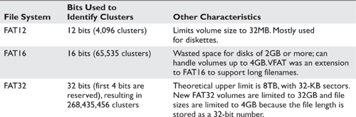
Table 6-1 FAT File System Characteristics (Source: FAT File System. Retrieved from http://technet.microsoft.com/en-us/library/cc938438.aspx.)
EXAM TIP Because of the inefficient use of space, some claim that FAT16 can only handle volumes up to 2GB.
NTFS NTFS (once “New Technology File System,” but now just plain ol’ NTFS) is fully supported only by Windows, although there are tools on Linux and Max OS X that will read from and write to NTFS file systems. NTFS supports 64-bit cluster numbers, and when combined with a 64-KB cluster allows volumes up to 16 exabytes (16 billion gigabytes), although practical implementations are effectively limited to 32-bit cluster numbers. The default cluster size for NTFS is 4KB when the volume size is over 2GB.
The heart of NTFS is the Master File Table (MFT). An MFT is constructed for each volume configured with an NTFS file system. Among its other capabilities, NTFS can compress files and encrypt single files or entire directory hierarchies.
Table 6-2 lists the elements of the MFT.5
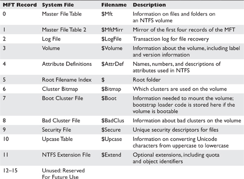
Table 6-2 NTFS Master File Table
Mac File Systems Mac OS X uses the Hierarchical File System (HFS) and HFS+. HFS+ was a modification to HFS that supported larger volumes sizes. HFS itself uses seven different data structures on disk to manage its file systems:
• The Volume Header starts after the first 1,024 bytes of the volume. It contains information about the date and time the volume was created and the number of files on the volume.
• The Allocation File indicates whether a particular block is allocated or free.
• The Extents Overflow File contains file extents (allocated file blocks) if a file is larger than eight extents, which are stored in the volume’s catalog file. A list of bad blocks is also kept in this file.
• The Catalog File describes the folder and file hierarchy. It is stored as a B-tree to allow speedy searches. It stores the file and folder names (up to 255 characters).
• The Attributes File stores additional file attributes.
• The Startup File is used to boot non–Mac OS machines from an HFS+ volume.
The end of the volume contains a second volume header that precedes the last 512 bytes of the volume—those bytes are reserved.
One thing to remember about Mac file systems is that files are composed of two “forks”: a data fork and a resource fork. The data fork stores what we normally think of as the contents of the file, while the resource fork stores such things as font files, language translation files, icons, and so forth. This file format has been superseded on other systems by a file type that appears as a single file, but is in fact an archive of files, each containing some aspect of the complete files. An example of this is the Microsoft Word .docx file. This file actually consists of several other files containing the text of the document and other information.
The Windows NTFS file system provides the capability for a user to create an alternate data stream (ADS). This capability allows you to attach one file to another, but the file that is attached is essentially invisible to normal directory listing tools. The file size of the original is the same as it was before the other file was appended.
Earlier versions of Windows (starting with Windows NT and later) would not show these files using normal directory listing tools (Windows Explorer and the dir command). In Windows 7, the dir command has a parameter (/R) that will list alternate data streams. We’ll have more to say about ADS in Chapter 7 when we discuss Windows forensics.
Linux File Systems File systems currently used in the Linux world include ext2, ext3, ext4, ReiserFS, Reiser4, and ZFS. Ext2 was the standard following the .ext file system, and ext3 and ext4 have extended its capabilities. Ext3 added journaling, and ext4 added the ability to address storage up to 1EB (exabyte) of data.
In Linux, a directory entry (dentry) consists of a filename and an inode (many files can refer to a single inode). Other objects in a Linux file system are superblocks, files, and inodes (the original reason for this name has been lost in the mists of time). The superblock is the first block on the disk (inode 1) and contains metadata about the file system. This block is important enough that a copy of it is stored at multiple locations on the partition. The inode holds the file’s metadata as well as a list of data block addresses. Depending on the file size, the inode can point to an indirect block where each entry is the address of a disk block that contains file data. This setup is called an indirect block, and it’s possible to have double- and triple-indirect blocks as well.
NOTE For the curious, the double-indirect block would have pointers to another indirect block that would itself have pointers to the actual data blocks. Triple-indirect blocks would add yet another set of pointers. Whew!
The ZFS File System The ZFS file system had its origins with Sun Microsystems and has recently appeared as an option for Linux computers. ZFS is short for Zettabyte File System, and as you may have guessed, it was created to handle large files. ZFS utilizes zpools that are in turn composed of vdevs that map to one or more physical devices, including RAID devices. Block sizes can range as high as 128KB, with 128 bits to number clusters: For the curious, 2**128 is 3.4028237e + 38, or more more specifically
340,282,366,920,938,463,463,374,607,431,768,211,456
Multiplied by the block size, of course.
The Sleuth Kit (TSK) is a set of open-source digital forensic tools overseen by Brian Carrier at www.sleuthkit.org. As described on their web site:
The Sleuth Kit™ (TSK) is a library and collection of command line tools that allow you to investigate disk images. The core functionality of TSK allows you to analyze volume and file system data. The plug-in framework allows you to incorporate additional modules to analyze file contents and build automated systems. The library can be incorporated into larger digital forensics tools and the command line tools can be directly used to find evidence.6
If you are approaching a file system analysis for the first time, three tools from the TSK stand out. fsstat displays details of a particular file system, including the range of metadata values (inode numbers) and content units (blocks or clusters). The layout for each group is listed, providing the underlying file system supports this notion (FFS and EXTFS). Figure 6-6 shows the output of fsstat when run on an image (istick.img) of a USB drive captured using the dd command.
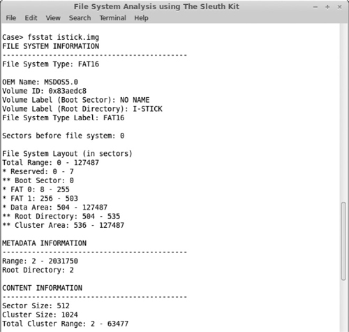
Figure 6-6 fsstat output
The fls tool lists allocated and deleted files in a directory. Figure 6-7 shows the (abbreviated) output of the fls command. Deleted files are highlighted in the listing.
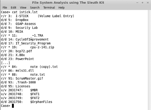
Figure 6-7 fls command output showing deleted files
Once you’ve determined the deleted file that you’re interested in, you can retrieve that file using the icat command, which writes the file to the standard output device (usually the terminal) or a file. Figure 6-8 shows the results of the icat command and the first few lines of the recovered file.
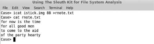
Figure 6-8 icat command output and file listing
How do I know what kind of file it is? Files can be identified by their file extension, by a “magic number” found at the beginning of a file, or by an identifiable pattern in the file structure. Microsoft Windows uses the file extension, whereas Linux looks for a “magic number” within the first file block of the file, or for a particular pattern. The Linux file command utilizes a database of specifications that can identify particular kinds of files.
All operating systems go through a similar process once the power is switched on. “It’s the same thing, only different” was never truer than in this case, and so it’s worth looking at each of the mainstream operating systems to detail the variations in each. “Booting” the system comes from the old adage of “pulling oneself up by your own bootstraps,” and this is exactly what the OS does. The general idea is to execute a small piece of code that exists in read-only memory (ROM) that loads the “bootloader “software. That software, in turn, does a little more and then hands the process off to yet more powerful and capable software, which may be the operating system itself or another bootloader.
The generic version of the boot process goes something like this. After power-on, the central processing unit (CPU) executes code from ROM that performs two steps: validate that all elements of the computer are working normally via a power-on self-test (POST), and load the OS into memory. These goals can be achieved by either a single program or multiple smaller programs (a multistage bootloader). Usually, the user is offered an option to choose a particular boot device or to use the default. Options include a hard disk, a CD-ROM drive, a USB device, or the network, where the local hard disk is the default. Choosing a CD-ROM drive or a USB device enables you to boot a computer using a different OS than what is installed on the machine’s installed drive (HDD or SSD). That drive is still discovered by the booted OS, but is not modified and can be mounted as read-only.
TIP Booting from a nonwriteable media such as a CD makes sense if you suspect that the machine may have some kind of malware installed that could affect the operation of the OS.
The MBR is the first 512 bytes on the chosen boot device and ends with two bytes 0X55AA (a boot sector signature). The MBR contains a master partition table that contains a complete description of the partitions that are contained on the storage device and the master boot code that acts as an OS-independent chained bootloader. Figure 6-9 shows the contents of an MBR on a Linux machine. You can retrieve this information via this command:
dd if=/dev/sda of=mbr.bin bs=512 count=1
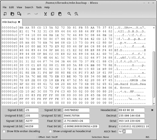
Figure 6-9 Contents of a master boot record
The basic input/output system (BIOS) reads the master boot code from the MBR and executes that code. That code indicates which volume bootloader to use in case the computer is configured to dual- or triple-boot into a different OS. It’s at this point that things start to get interesting.
As a DFI, you will encounter many different operating systems in the field, and many of them will be running some version of Windows. As of this writing, the newest version of Microsoft Windows is 8.1, but you may encounter 7, Vista, and XP Service Pack 3. Windows XP and earlier had one type of boot process; Vista and later versions have another.
Windows XP Service Pack 3 The first stage of the process for booting Windows XP is starting the ntldr program that loads system device drivers so that it can load files from any supported file system type. If a boot.ini file exists, ntldr will read that file and display a menu of options. If the chosen OS is Windows XP, ntldr will load the ntdect.exe file to choose a hardware profile. The second stage is the ntoskrnl, which proceeds as follows:
• Starts all executive subsystems.
• Loads and starts the I/O manager and then starts loading all the system driver files as well as the smss (Session Manager Subsystem).
• The smss loads the win32k.sys device driver. At this point, the screen is switched into graphics mode. The winlogon.exe program starts the login process, and the local security authority (lsass.exe) processes the logon dialog box.
Windows Vista and Later Later versions of the Windows OS have a slightly different procedure. Instead of ntldr, the boot code invokes the Windows Boot Manager (bootmgr) that reads and executes instructions from the boot configuration data file. The first instructions are a set of menu entries that allow the user to choose whether to boot the OS via our old friend winload.exe, resume the OS from hibernation, boot an earlier version of Windows (via ntldr), or execute a volume bootloader. The boot configuration file can be edited by various programs, one of which is bcdedit.exe, and can boot third-party software. This is one point where the suspect could have modified Windows startup to invoke software that would obliterate evidence.
Winload.exe then starts by loading the OS kernel (ntoskrnl.exe) and other device drivers required at this point in the boot process. Once the OS kernel is loaded, the process is much like what happens in Windows XP and earlier.
EXAM TIP The stages of the Windows XP boot process are ntldr, ntoskrnl, smss, WinLogin.exe, and lsass.
MBRs have been around for a good long time, as has the BIOS that provides the bootstrap code. Since 2010, a newer specification, the Unified Extensible Firmware Interface (UEFI), is gradually advancing, driven by Microsoft’s announcement that Windows 8 computers would need to use it. UEFI has several improvements over the BIOS. Microsoft7 describes these advantages as follows:
• Better security by helping to protect the pre-startup—or pre-boot—process against bootkit attacks
• Faster startup times and resuming from hibernation
• Support for drives larger than 2.2TB
• Support for modern, 64-bit firmware device drivers that the system can use to address more than 17.2 billion GB of memory during startup
• Capability to use BIOS with UEFI hardware
The key to understanding the UEFI specification as it relates to persistent storage is the notion of a GUID partition table (GPT). The GPT replaces the MBR for disk partitioning. Some OS tools already understand the structure of the GPT and are able to both recognize and create a partition of this type.
For the DFI, the GPT represents an opportunity for the technically adept suspect to hide data in yet more places, as well as providing more places for malware to hide. Fortunately, it appears that creating a forensic duplicate of a drive using the GPT format will contain all the necessary data as a drive that uses an MBR.
TIP In order to support legacy systems, a drive that uses the GPT format will create an MBR sector that indicates that the drive is full. The experienced DFI will know to check for the presence of the GPT.
Compared to Windows, Linux is simplicity itself. The BIOS reads the master boot record and loads either LILO (Linux Loader) or GRUB (Grand Unified Bootloader), although GRUB 2 is now increasingly common. Either of these will ask the user to choose a particular OS. Once chosen, the boot loader will start the operating system and hand off control. The OS will look for the init program and start it (init is the parent of all processes that start up automatically). init then reads the file /etc/inittab and executes commands listed within that file for a particular OS state called the run level. Successful execution of programs at a particular run level allows the system to transition to a higher run level.
Mac OS X is closer to Linux than to Windows given that at the command line, at least, Mac OS X is based on a Berkeley Systems Division (BSD) version of UNIX.
NOTE Strictly speaking, Mac OS X runs a BSD “personality” on top of the Mach microkernel.
The boot process for Mac OS X is less readily understood because it uses Open Firmware. Open Firmware is the first program executed when the machine is powered on, and is a good place to stop and examine the configuration of the computer (provided you’re familiar with the Open Firmware command set). The firmware loads the BootX loader, which goes through a number of hardware configuration steps, the last of which is to determine if the OS kernel is compressed, whether it is a “fat binary” (contains code for Intel and PowerPC processors), and whether it is Mach binary or an executable and linking format (ELF) binary. If all goes well, BootX will load the OS kernel. The kernel, in turn, starts its init that performs some Mach-specific tasks and then starts the /sbin/init process. The rest of the startup process that follows is virtually identical to the Linux boot rprocess. The last step in this process is to start /sbin/Systemstarter, which starts up configured startup items (/System/Library/StartupItems and /Library/StartupItems). The login application, loginwindow.app, starts, and the user can log in to the running system.
The primary issue with the boot process of any device is determining which programs run during initial system startup. A suspect may include code as part of this sequence that will destroy evidence related to their activities. The autoruns program from the SysInternals folks at Microsoft will list all the programs that are scheduled to run when the system is started. In Linux, it’s easy enough to check the entries in the /etc/rcN.d directories (which in turn should be symbolic links back to programs in the /etc/init.d directory). In Mac OS X, inspecting the files in /Library/StartupItems and /System/Library/StartupItems can provide a hint as to whether additional software has been installed.
Since you can configure a computer to choose a different boot device (a CD-ROM, USB drive, first hard disk, or the network), you can easily boot a device from a CD-ROM or a USB key that can run an alternative operating system. Several forensic distributions are distributed as a “live” distribution that can be run directly from a CD-ROM, with the OS entirely in memory, or from a USB device that offers the ability to save data to that drive. Once the forensic software is operating, the disk of the suspect’s computer could be mounted read-only.
Another technique is to use a forensics distribution provided as a virtual machine image. These images can be executed by VMware Workstation, VMware Player, or VirtualBox. External devices can be attached to these VMs and examined by the forensics software.
We’ve just spent the preceding section talking about the physical and logical layout of a disk drive. We have to take into account what happens when certain elements are removed or deleted from a file system. What happens when someone deletes a partition? What happens when someone deletes a file? Both of these actions can take place intentionally or unintentionally. If a file or partition is deleted accidentally, we’re in the realm of data recovery. If it’s done deliberately, then we’re in the realm of forensic data recovery.
NOTE I recall when a colleague of mine wrote over the partition table of a disk containing another colleague’s Ph.D. thesis research—raw data, results, software developed as part of this research—everything. Although the situation turned out okay (files could be recovered), there were some extremely anxious moments and two very distraught people.
One difference between data recovery and forensic data recovery is that in forensic data recovery, we are much more interested in the modified/accessed/created (MAC) times of the deleted file. Establishing the time at which the file or partition was deleted becomes part of our forensic timeline analysis. For data recovery, we may be interested in a larger block of time (“I deleted that file last Tuesday late in the afternoon—between 4:00 and 6:00 P.M.”).
As we saw earlier, disk partitions are laid out in a partition table that occupies the first 512 bytes at offset 0 of the disk. When a partition is deleted, it means that the space is reallocated to another partition, or effectively becomes unavailable because it is no longer recognized by the host OS. That doesn’t mean that the data on that partition are gone forever; rather, it means that those clusters are now unavailable to the disk as a whole until the partitions are reconfigured.
If a partition is hidden, that partition is no longer visible to the end user. The OS is aware of this partition, but it won’t list it on any of the standard desktop tools. Unhiding a partition is relatively easy using the system tools provided with your OS. For instance, you can unhide a partition by unsetting the “hidden” flag that is set in the partition header on some systems. On Windows, you can hide a partition by using the diskpart program to remove the drive letter assigned to the partition. Select the appropriate drive and issue the command “remove drive e:”. You can also manipulate a registry key, HKEY_CURRENT_USER\Software\Microsoft\Windows\CurrentVersion\Policies\Explore, to indicate which partitions are logically hidden to Windows Explorer and other software. Create a new DWORD value named NoDrives for that key, and enter a value that represents a bit mask to indicate which drive letters should be ignored (drive A is 1, drive B is 2, drive C is 4, drive D is 8, and so on up to drive Z). And yes, you can combine the values: A value of 3 would ignore drives A and B.8
Various programs can manipulate partition tables. One of my favorites is gparted (Gnome Partition Editor), a graphical version of the Linux commands parted and fdisk. Windows offers Partition Magic, a third-party solution, as well as diskpart and diskmgmt.msc (both native Windows software). Figure 6-10 shows the user interface to the gparted command.

Figure 6-10 gparted user interface
Recovering deleted disk partitions is always one of my favorite jobs. Fortunately, there are multiple software tools to help you in that task. The testdisk software is multiplatform, and runs on Windows, Mac, and Linux. It searches for deleted partitions by looking at each physical sector on the disk and determining if it contains a file system. The gpart software is Linux only, but it’s included on several bootable Linux distributions such that it can be applied to an ailing HDD. You can use the Mac’s Disk Utility software to create and delete disk partitions.
Once we have a usable partition, we can anticipate recovering deleted files on that partition. This assumes that we can’t use the simple way: retrieve the file from backup.
TIP Asking about automatic backups of employees’ drives can make file recovery a lot easier. Likewise, check TimeMachine on a Mac and Restore Points or Volume Shadow copies or Volume Shadow copies on a Windows machine.
However, if we’re talking about an individual, it’s a rare bird that actually systematically backs up data to a remote drive or location such as Mozy, Carbonite, Dropbox, or Box, so we’re faced with recovering the file from the storage medium.
When a file is deleted, different things happen, depending on the OS running on the suspect’s computer. In Linux when a file is deleted, the disk blocks associated with the file inode (index node) are returned to the list of free disk blocks for reuse. How the file is represented as deleted may vary: The inode value in the directory may be set to zero, or the entry can be deleted completely from the directory file.
In Windows, what happens depends on the type of file system. If the file system is formatted using some type of FAT file system, then several things happen.9
1. The first character of the filename is changed to 0xEH.
2. The file is moved to the Recovery Bin directory (C:\RECYCLED for FAT file systems, C:\RECYCLER\S-… in NTFS, or $RECYCLE.BIN in Windows 7). For NTFS, each user is provided with a subdirectory in the C:\RECYCLER directory named with the Windows security identifier (SID). On my computer, my SID is S-1-5-21-1145031325…-1005, and I can observe a subdirectory C:\$RECYCLE .BIN\S-1-5-21-114…-1005.
3. The file is moved to the recycle directory and renamed using the following strategy:
a. First letter of the new filename is D.
b. The second letter is the drive letter for the source of the file (say, E:).
c. The next numbers are the sequential number of files that have been deleted from the drive. DE01.pdf would be the second file deleted from the E: drive.
4. Information about the file is written to the file INFO2. The INFO2 file contains the details of the original file, say, E:\documents\Guidance.pdf.
At that point, the file can be deleted from the Recycle Bin, in which case the associated disk blocks are returned to the system for reuse, or the file can be restored to its original location that has been previously saved in the INFO2 file. Mac OS X, via the Finder, operates in a similar manner, with Trash taking the place of the Recycle Bin.
EXAM TIP Understand how files are renamed in the Recycle Bin and what information is stored in the INFO2 file.
So how do we recover a file? The simple answer is that we find the clusters that were allocated to the original file and relink them to a file that we create in a specified location. Moreover, we’d like to do this without changing any of the original file’s metadata in order to preserve our timeline.
Some of the metadata that we’re interested in regarding files are the times when the file was modified, created, or accessed (the MAC times). These times depend on the OS you’re running and the action that you performed. You might think that accessed time would be straightforward: It’s the time I last “read” the file. But does that include the last time you listed the contents of the directory?
Directories (and subdirectories) are also files, although a different kind of file. If I delete a subdirectory, all regular files contained in that directory must be deleted prior to deleting that subdirectory, and all subdirectories must be deleted as well. The user must explicitly request deleting a directory hierarchy, due to the damage that can result (consider the effects of inadvertently typing del Documents in your home directory on a Windows computer).
As expected, there are different tools for different OSs, some that are cross-platform, dozens to choose from, and more developed every day. How to choose? Michael Graves lists four criteria for choosing third-party tools:10
• Accuracy
• Verifiable output
• Consistency
• Usability
Assuming that a tool meets these four criteria, the next consideration is whether the tool meets the tests established by the Daubert11 process. Michael Graves summarizes these tests thusly:12
• Can the evidence presented be, or has it been, tested empirically, and can it be verified?
• Has the approach or technique been the subject of peer review and publication?
• Is the technique generally accepted within the scientific or professional community?
• Does the technique or procedure contain a high known or potential rate of error?
The choice comes down to personal preference and the ease of accessing features you use most often. Frankly, some software tools just seem to “fit” better than others do. I’ve listed my personal favorites next for each of the major operating systems, but they may not be yours.
I’ve used gparted on a live CD to repartition and fix a balky Windows system that mysteriously lost its boot drive. I’ve also used diskmanagement.msc to delete and expand partitions, and I’ve used the Undelete software to manage file deletions on my work computer.
DiskWarrior saved my Mac Mini when I powered off the machine before it had completed shutting down. None of the available Mac recovery tools would work, but DiskWarrior was able to fix the problem, as well as cleaning up other small inconsistencies in the file system.
I’ve used gpart, gparted, and testdisk to recover my HDD when I typed /dev/sdb instead of /dev/sdc, and instead of overwriting the MBR on a USB disk, I overwrote the MBR on the boot disk. Testdisk ultimately came to my rescue.
TIP On Linux, you can create a makeshift Undelete facility by aliasing the rm command to instead mv or cp the selected files to a new directory named Recovery Bin or something similar. If “deleter’s remorse” sets in, it’s easy enough to go to the Recovery Bin and retrieve the mistakenly deleted file.
Regardless of whether we have undeleted or recovered a graphics file, that file can be used to hide information that could be evidence in our investigation. We previously defined a graphics files as a file that can be rendered as a graphic image using appropriate software. Given that “image” is another overloaded word in the computing industry, I’m going to refer to these files as graphics files from now on.
There are multiple graphics file formats from which to choose. A single photographic image can be represented by multiple graphics file formats, although they don’t all offer the same features or quality.
There are two major types of graphics: raster and vector. Raster graphics represent each pixel as a bit-string, organized in rows. Displaying these files requires reading each of the values and reflecting them onto the monitor screen. Vector graphics represent an image as a series of equations, which allows the file to be expanded without losing detail.
Table 6-3 summarizes the most common file formats.
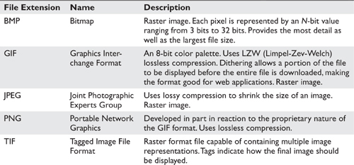
Table 6-3 Graphics File Formats
Metafile graphics files contain both raster and vector images. Enlarging this file will cause the image displayed to lose detail in the raster portion, but the vector images will display at full detail.
All graphics file formats contain metadata. Figure 6-11 shows the metadata associated with a photograph.

Figure 6-11 Photograph metadata
This is a good time to take a small detour to talk about graphics file compression. Graphics files can be large. The greater the number of pixels, the larger the file (one pixel is represented by up to 32 bits of data, allowing over 4 billion colors). Compressing these files can save storage space and decrease the time needed to send these files over a communications network. Unfortunately, compression algorithms are not created equal. Lossless compression means that a compressed file can be restored to an exact representation of the original. Lossy compression means that the file cannot be restored to its original, but can provide a “good enough” representation.
Some graphics file formats already compress the image, using either LZW or Huffman encoding. Huffman encoding is a fixed- to variable-length encoding scheme that provides lossless compression, and does so by assigning short codes to characters that appear frequently and longer codes to characters that appear less frequently. Consider the letter e 0 × 45 which is the most used letter in the English alphabet. Huffman encoding might assign that letter a code of 0b0, while the letter z might be assigned the value of 0b1001011. Compression is thus achieved by replacing common bit strings with shorter ones that shorten the length of the file. LZW is a variable- to fixed-length encoding scheme that also provides lossless compression. It creates a dictionary of nonoverlapping bit strings and then replaces these strings in the file with code that represents the bit strings.
The JPEG format provides lossy compression, in that a file stored as a JPEG image is compressed by ignoring less critical elements of the original image. Vector quantization is a technique whereby certain strings of bits are represented by their average value, analogous to replacing the string of values “123123” with the value 5. Lossy compression is never used on text, since replacing a string of characters with an approximate value results in gibberish, at best, and horrible miscommunication, at worst (consider the effects of changing the “2” to a “5” in the message: “We attack at 2pm tomorrow”).
Image file compression is distinct from file compression. File compression software must be nonloss; examples of file compression software include Zip, 7-Zip, RAR, GZIP, and BZIP. From a privacy perspective, a compressed file is almost as good as an encrypted file, since the compressed data are unintelligible if simply viewed from a binary editor and would be unreadable by a program unless the data are decompressed.
Some file compression software supports encrypting the file as well. This requires that the file be compressed prior to encrypting, since compressing an encrypted file shouldn’t find any repeated character sequences that can be expressed as a value and a length.
As we mentioned earlier when discussing the encrypting file system (EFS) on Windows, if you are running live on the host OS, a compressed file created via that OS will be uncompressed for you when read (and decrypted as well). Running on an image capture of a disk is another matter, since neither the decompression algorithm nor the encryption key may be known to your forensics OS. This is equally true if the file has been encrypted when the file system itself (or portions of it) have been automatically encrypted by the OS.
Recall that we can determine the type of a file via either the file extension or a “magic number” that is embedded into a particular file type. Renaming the file with a different file extension will probably mean that the software that created the file won’t think that it can read the file and various search programs may overlook it, especially when searching for graphics files. We can use this technique to “carve” or “salvage” graphics files from a damaged disk or from unallocated space if the graphics files have been deliberately deleted or corrupted. If the file header has been corrupted, it can be fixed by using a disk/binary file editor by either changing its contents or adding any missing information.
Imagine you’re performing a file system analysis and you retrieve a file with no extension. No software on your computer recognizes the format. How might we go about identifying that file?
The answer is similar to how we locate and recover graphics files. First, we look for file signatures using, say, the Linux file command. The file command uses a set of heuristics to determine what kind of file it might be, and these heuristics are based on fixed patterns in particular kinds of files. The strings command from the Sysinternals suite would let us examine any ASCII or Unicode sequence of characters that might help us identify the file type.
Conversely, if you have a file extension but you have no idea what program created this particular file or how it’s formatted, using a resource like www.filext.com to identify the extension and its creators can save you valuable time. Other software, such as IrfanView and ACDSee, will attempt to determine the actual file format when opening a file. Using a multipurpose viewer like Quick View Plus can also save time and the expense of obtaining the actual software used to create that file.
Steganography is the general practice of “hiding” data within a cover medium, sometimes called a “host file.” This file can be any kind of file, really, although usually it’s a graphics file. While there are different methods of steganography, what they all share is an abstract view of a stegosystem. A stegosystem is composed of a message embedded in the cover medium along with a stegokey. Taken together, these three items create a stegomedium. The recipient of this medium will use the stegokey and the stegomedium to derive the (embedded) message.
NOTE This description sounds very much like encrypting a digital object, and the message sounds a lot like a watermark. We’ll compare all three later on in this chapter.
EC-Council lists two examples of steganography that aren’t malicious.13 Medical records can have a patient ID inserted within them to make sure that the information applies to a particular patient, even if other identifiers were lost or modified. Steganography can be used in the workplace to keep communications private that concern intellectual property: For example, details of a secret project could be communicated among project members without leaving a “paper” trail. Steganography is useful in any circumstance when we wish to incorporate extra information in a particular digital object such that a casual observer wouldn’t know that information is being exchanged.
The EC-Council lists three major methods of steganography: technical, linguistic, and digital.13 Technical steganography uses an outside medium, such as chemicals or liquids, to reveal the hidden message. One example of this kind of steganography is the time-honored technique of writing a message using lemon juice and milk, and then exposing the paper to low heat to reveal the message.
Linguistic steganography consists of two types: semagrams and open codes. Semagrams either can be visual, such as arranging objects to communicate the message, or can use variations in font, spelling, and punctuation to embed the message in a plain text file.
Open codes modify plain text files to send the message. One technique uses argot codes, where information is communicated via a language that only the participants can understand. Another is covered ciphers, where the message is embedded within plain text, but only the receiver knows how to extract the message. The null cipher embeds the text of the message in the host file according to some pattern, such as the first word of each sentence, the first letter of every third word, vertically, horizontally, and so forth. Grille ciphers require a special form or template to be placed over the text that reveals the letters or characters of the message. No grille, no message.
Digital steganography hides messages in a digital medium, which is to say graphics files, audio, video, and so forth. The EC-Council lists the following techniques used in digital steganography:14
• Injection
• Least significant bit (LSB)
• Transform-domain techniques
• Spread-spectrum encoding
• Perceptual masking
• File generation
• Statistical methods
• Distortion technique
We can categorize these techniques as belonging to one of two strategies: insertion, where we include that message with the host file, and substitution, where we replace bits of the host file with bits from the message.
Steganography Methods in Text Files As we might expect, we can apply several steganographic techniques to hide a message within a text file.13
• Open space steganography uses the presence of white space within the text (either blanks or tabs), whether as intersentence spacing, end-of-line spacing, or interword spacing.
• Syntactic steganography uses the presence or absence of punctuation characters to represent one and zero. A comma could represent a one; the absence of a comma could be interpreted as a zero. The sequence “a,b,c a b c” could be decoded as “11000.” In this instance, letters don’t matter, only the punctuation, so we’re left with comma, comma, and three spaces.
• Semantic steganography uses two synonyms, one of which is declared primary and one secondary. The appearance of the primary synonym is read as a 1; the secondary synonym is read as a 0. For example I might use the phrase “party” as the primary synonym and the phrase “event” as the secondary.
As with any steganographic technique, the receiver must know how the secret message is included in the text in order to retrieve it.
Steganography Techniques in Graphics Files Messages can be hidden in graphics files by using LSB insertion, masking and filtering, and algorithmic transformation. The LSB technique is used for other media as well as graphics. In this technique, the LSB of, say, a 24-bit quantity would be replaced with bits from the secret message. In the case of graphic files that utilize 24- or 32-bit color, the resulting changes would not be discernible to the viewer. In contrast to techniques like open space steganography, LSB encoding, algorithmic techniques, masking, and filtering all represent a substitution approach.
Steganography Techniques in Audio Files A suspect can hide messages in audio files using variations on the LSB technique or by manipulating various frequencies. Techniques include phase coding, spread spectrum, and echo data hiding. Phase coding separates the sound into discrete segments and then introduces a reference phase that contains the information. Spread spectrum techniques encode the information across the entire frequency spectrum using direct-sequence spread spectrum (DSSS). Echo data hiding means introducing an echo into the original medium, and properties of the echo are used to represent information.
Steganography Techniques in Video Files Messages can be hidden in video files using any technique that applies to audio or graphic files (a video is an audio stream overlaid on a series of images). One such technique is modifying the coefficients used in the discrete cosine transform (DCT) computation, a technique used to compress JPEG files, so as to hide parts of the messages in areas of the file that will survive expansion and recompression.
Steganographic File Systems Steganographic file systems encrypt and hide files inside of random blocks allocated to that file system, but keep just enough information available to re-create these files when presented with a filename and a password. To an outside observer, the disk seems to be a collection of random bits that appears to be nonsensical when read. One implementation is the StegFS file system for Linux. StegFS is described as
[…] a steganographic file system that [… offers] plausible deniability to owners of protected files. StegFS securely hides user-selected files in a file system so that, without the corresponding access keys, an attacker would not be able to deduce their existence, even if the attacker is thoroughly familiar with the implementation of the file system and has gained full access to it.15
Steganography, watermarking, and cryptography are ways of concealing the content of a message or a file such that only someone who knows the secret can retrieve that information. Nevertheless, there are significant differences among these techniques. Cryptography modifies the file in such a way that the contents are unintelligible to the software that is used to display that file. Steganography, however, inserts the secret contents into a file such that the contents can be extracted or viewed or read by the appropriate software, and the original file can still be read or displayed.
Here’s an example. I want to send to a message to my friend Sam that says, “You and Barbara should meet us at the restaurant at 8:00 P.M. tonight. It’s a surprise party for Helyn.” I don’t want anyone else to view that message (I want to keep the party small), so I encrypt it and send it to Sam. I’ve made the encryption key available to Sam via some other means, so Sam can use the encryption key to decrypt the file and view the message.
However, if I have reason to believe that sending an encrypted file might cause suspicion (or might be specifically forbidden by company policy), I could use steganography to embed that message in the photograph and then send the modified photograph to Sam. Anyone viewing the photograph might see a travel snapshot, but Sam, who has the stegokey, can extract the message from the photograph and hopefully join us in the festivities.
Watermarking and steganography differ in that watermarks can be either visible or invisible. Visible watermarks are meant to be clearly seen and to require a good deal of work to remove. The goal of invisible watermarks is to remain hidden from the receiver, but be visible using software in the possession of the creator, who can make the watermark visible by knowing the watermark password. This technique is used to track illegal copies of documents and to ensure that copyright laws are followed. An example of this technique is to release a set of the same document that contains different watermarks. If the document shows up in the wrong hands, the sender can retrieve the watermark to learn the source of the leak.
The major differences between watermarking and steganography in that watermarking is ultimately meant to be seen, whereas in steganography, the secret message is meant to remain hidden such that only specific individuals will be able to retrieve it from the carrier file. Cryptography is similar to steganography in this regard, but using cryptography means that everyone can tell that the content of the message is hidden, whereas in steganography, the carrier file appears to be normal.
Steganalysis is the practice of analyzing a file to determine if it contains information encoded as part of the data portion of the file. It is the process by which we attempt to determine if steganography is present and, if so, to determine the stegokey and the method used to embed the message in the host file.
Kerckhoff’s principle in cryptography states that the only thing that must be secret is the key itself: The encryption algorithm can be safely published. Steganography, however, needs to keep the stegokey secret, and requires that the sender and recipient must have the same software tool. The presence of steganography software on a suspect’s computer is a good indicator that communications sent or received by the suspect may use steganography. Tools are available that can make an educated guess at whether a particular file contains steganography, but they can’t actually extract the embedded message.
How can we detect steganography? That part is not so easy. In many cases, the naked eye just can’t distinguish between the original graphic and the modified graphic. The simplest way is to obtain a copy of the original image and compare the two files using a simple file comparison utility such as comp on Windows. Differences between the two may indicate the presence of steganography (determining which is the original, however, may be more of a problem), or it can mean a change in file metadata similar to what we saw in the metadata associated with a photograph. Change the location setting in the photograph metadata, and we’ve changed the file signature.
Two general approaches for detecting steganography are the statistical and empirical methods. In statistical analysis, we can use a tool that measures the entropy (variability) of a particular document. Files that contain a hidden message should have more entropy than the original. Empirical approaches involve examining files directly. If we are looking at images, we can look for changes in file size, modified date, or the color palette used. If we are examining text files, we can look for such things as abnormally large payloads (data portions of a message), as well as a lot of extraneous white space.
As a DFI, you’re more interested in viewing the contents of a graphics file than in changing the background to a different color. If that’s all you need, acquiring software like Adobe Photoshop or the GIMP (GNU Image Manipulation Program) would be overkill. There are many software tools that you can use to view images, some free of charge and some commercial. Viewing images is not the same as modifying (editing) those images. Two things that I look for in software is the ability to display different kinds of graphics files as well as displaying file metadata.
IrfanView is a free-as-in-beer software (but the author would appreciate your buying him a virtual beer now and again). Figure 6-12 shows the user interface for the software. Notice that the software is able to extract metadata from the file.
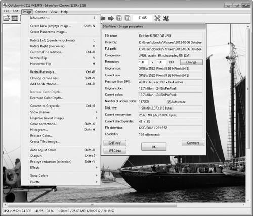
Figure 6-12 IrfanView user interface
QuickView Plus handles multiple image formats as well as popular office documents (the Professional version will even open Microsoft Project files). Although versatile and expansive in terms of the number of file formats it can interpret, QuickView Plus doesn’t provide the capability to inspect file metadata. Get the picture?
Likewise, there are many sources for graphics file forensic tools. Examples include Hex Workshop and Ilook. Figure 6-13 shows Hex Workshop after it’s opened the same file we previously opened with IrfanView. As it happens, IrfanView can be configured to use Hex Workshop (or any other editing tool) to examine the raw bytes comprising that file. The ability to hook individual software programs together or to extend a tool via scripting language is a feature well worth having.
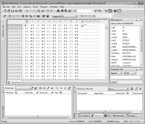
Figure 6-13 Hex Workshop view of the graphics file
Steganography is difficult to detect, and even harder to extract when discovered. Several tools will look for files that have hidden messages, and while they can tell you that a given file may contain hidden content, they usually can’t help you in determining what that content is. Some tools will scan for known steganography software: The very presence of such software may provide a clue for conducting a deeper analysis of files on the suspect’s computer or for files that may have been sent via other means (file transfer, e-mail, text, instant message, and so on).
There is a world of choice for steganographic tools: One web site lists over 100.16 Some of the more noticeable tools are stegdetect and the S-Tools suite. stegdetect can discover several different steganographic techniques, and stegbreak implements a dictionary attack against three of them (Steg-Shell, JPHide, and OutGuess 0.13b). S-Tool is a single program that allows files to be embedded into a .gif, .bmp, or a .wav file. Although the program is getting a bit long in the tooth (the help file talks about running the software in Windows 95!), the software happily inserted a text file into a .gif and restored the text from the modified image.
MATLAB is a “high-level language and interactive environment for numerical computation, visualization, and programming,”17 and has been used for multiple applications, including processing video and images. Over time, the MATLAB software package became used to analyze forensic images. The general case is to utilize specific algorithms that can detect certain kinds of transformation that indicate that the digital image has been modified in some way, either to hide a message (steganograph) or to include or exclude data from the original. One example is using MATLAB to analyze the position of light sources in a photograph to determine if certain elements of the photograph have been added (often referred to as having been PhotoShopped, in recognition of the popular image manipulation software sold by Adobe, Inc). The author of the blog post “MATLAB in Forensic Image Processing”18 makes the claim that MATLAB is a good tool for forensic image processing because you can record every step of your analysis as well as examine the source code for the various algorithms used. This information can then support your analysis if challenged in court.
Hard disk drives consist of a spindle with rotating platters and read/write heads. Each disk has a number of tracks (concentric circles on the disk platter), and each track is divided into sectors. Each sector (block) can be addressed by an LBA; a file system block or cluster is a group of disk sectors that are allocated together for a file. Disks are usually formatted into multiple partitions that provide a logical volume name for a collection of disk blocks. RAID technology supports assigning multiple physical devices to a single logical volume. RAID uses striping, mirroring, and parity to provide availability and response time.
File systems are data structures that present a hierarchical view of storage to the end user. Files are stored in directories that can contain subdirectories. Different file systems support different disk sizes and provide different file metadata, although all provide timestamps that indicate when a file was created, modified, or accessed. File systems include FAT32, NTFS, ext3, ext4, HFS+, and ISO9660 for CD/DVDs.
All computer systems go through a process of “booting” when they are powered on. Although the steps vary, most systems will run a POST test to ensure that configured hardware is present and working, and then load a bootstrap loader that loads and starts various device drivers. The bootstrap loader then reads a second-stage loader into memory, which in turn loads and starts the operating system, which ultimately results in a login prompt or the server becoming operational.
Deleted files and partitions can be recovered by multiple means. In the case of files, disk resources formerly allocated to that file are still available from the unallocated space list. Deleted partitions can be recovered by modifying existing partition tables to reflect the presence of the deleted partition.
Image (graphics) files come in multiple formats, but a graphics file can use vector graphics, bitmapped graphics, or both. Bitmapped graphics are usually lossless, while some vector graphics formats can lose detail (JPEG files).
Steganography is the practice of hiding a message with a cover file by using steganographic software along with a stegokey. The recipient can use the software and the stegokey to retrieve the message from the carrier file. Steganography can be used to embed a message in a text file, a graphics file, a video file, or an audio file. Steganography is difficult to detect and even more difficult to extract the message from the carrier file. Tools exist to analyze files for the presence of steganography, but without the software that was originally used to create the carrier file and the stegokey, it may be too time consuming to continue.
1. Tracks at the same position on each platter create what kind of structure?
A. Clusters
B. File blocks
C. Cylinders
D. Logical volumes
2. What strategy does RAID 10 use?
A. Volume data are striped, and each stripe is mirrored.
B. Logical volumes are mirrored and each mirror is striped.
C. Logical volumes are mirrored, and parity is stored within each disk.
D. Logical volume data are striped with a single parity disk.
3. A file system block or cluster is composed of a number of:
A. Tracks
B. Sectors
C. Cylinders
D. Platters
4. Which FAT version can only support disks up to 2GB in size?
A. FAT12
B. FAT16
C. VFAT
D. FAT32
5. Which of these elements make up the MAC time of a file? (Choose all that apply.)
A. Modified
B. Accessed
C. Created
D. Copied
6. What strategy does the testdisk software use to discover deleted partitions?
A. Compares MBR partition table entries to logical disk blocks
B. Looks for the last cluster in a cluster chain
C. Looks for file systems
D. Looks for partition table signatures
7. Which record in the MTF would have been damaged if I couldn’t tell which file blocks were in use?
A. Volume
B. Cluster bitmap
C. Boot cluster file
D. Root filename index
8. Which of these are methods to detect steganography? (Choose all that apply.)
A. Statistical
B. Empirical
C. Detective
D. Authentication
9. Two techniques used to compress graphics files are Huffman encoding and _______.
A. ZIP encoding
B. LZW encoding
C. 7bit
D. Radix64
10. Which one of these definitions best describes steganalysis?
A. Examining digital objects to discover embedded information
B. Comparing and contrasting the capabilities of steganography software
C. Building personality profiles of criminals who might use steganography
D. Deriving the stegokey from an analysis of the cover file
11. What are legitimate uses of steganography? (Choose all that apply.)
A. Record information in patient records
B. Intraoffice communication
C. Encoding manufacturing formulas for transmission
D. Sending URLs for contraband material
12. In Windows XP, the ______ is responsible for loading the operating system into memory.
A. ntldr
B. Winlogin
C. smss
D. lsass
13. File _____ is the process where we reclaim a graphics file from a raw disk.
A. Analysis
B. Resuscitation
C. Carving
D. Extraction
14. In order to extract the message from the stegomedium, the receiver must have the _____.
A. Symmetric key
B. Stegokey
C. Private key
D. Stegomask
15. The process of detecting the use of steganography is known as ____.
A. Steganalysis
B. Cryptanalysis
C. Stegodetection
D. Cryptography
1. C. Cylinders
2. B. Volume data are mirrored, and each mirror is striped across multiple disks.
3. B. Sectors
4. A. FAT12
5. A, B, C. Modified, accessed, and created
6. C. Looks for file system information
7. B. Cluster bitmap
8. A, B. Statistical and empirical methods
9. B. LZW encoding
10. A. Examining digital objects to discover embedded information
11. A, B. Recording information in patient records and intraoffice communication are both legitimate uses of steganography
12. A. ntldr
13. C. Carving
14. B. Stegokey
15. A. Steganalysis
1. Carrier, B. File System Forensic Analysis (NJ: Pearson, 2005), p. 10.
2. Evan-Amos, http://en.wikipedia.org/wiki/File:Laptop-hard-drive-exposed.jpg, licensed under the Creative-Commons Attribution-Share Alike 3.Unported, http://creativecommons.org/licenses/by-sa/3.0/deed.en.
3. Carrier, p. 70.
4. Afonin, Y. G. Why SSD Drives Destroy Court Evidence, and What Can be Done about It: Part 2. Retrieved from www.dfinews.com/articles/2012/10/why-ssd-drives-destroy-court-evidence-and-what-can-be-done-about-it-part-2.
5. Microsoft, 2010. The NTFS File System. Retrieved from www.technet.microsoft.com/en-us/library/cc976808.aspx.
6. “Overview.” Retrieved from www.sleuthkit.org/overview.
7. What is UEFI. Retrieved from http://windows.microsoft.com/en-us/windows-8/what-uefi.
8. NoDrives. Retrieved from http://technet.microsoft.com/en-us/library/cc938267.aspx.
9. “How the Recycle Bin Stores Files.” Retrieved from https://support.microsoft.com/kb/136517, retrieved June 23, 2014.
10. Graves, M. Digital Archaeology (NJ: Pearson, 2013), p. 399.
11. Daubert v. Merrell Dow Pharmaceuticals, Inc., 509 U.S. 579, 593 (1993).
12. Graves, Digital Archaeology, p. 401.
13. EC-Council. Computer Forensics: Investigating Data and Image Files (MA: Cengage, 2010), p. 1:9.
14. EC-Council. Computer Forensics: Investigating Data and Image Files (NJ: EC-Council, 2010), pp. 1–5.
15. HweeHwa Pang, Kian-Lee Tan, and Xuan Zhou, “StegFS: A Steganographic File System,” 19th International Conference on Data Engineering (ICDE ’03), Bangalore: IEEE Computer Society, 2003, p. 657. Abstract retrieved from www.computer.org/csdl/proceedings/icde/2003/2071/00/20710657-abs.html.
16. Johnson, N. “Steganography Software.” Retrieved from www.jjic.com/Steganography/Tools.htm.
17. Home page. Retrieved from www.matlab.com.
18. Unknown author. MATLAB in Forensic Image Processing. Retrieved from http://draftingschool.org/matlab-in-forensic-image-processing.