4
Water Quality

Claude E. Boyd and Craig S. Tucker

---

CHAPTER MENU

• 4.1 Introduction
• 4.2 Water Quality Variables
• 4.3 Effects of Water Quality on Aquatic Animals
• 4.4 Pond Water‐Quality Management
• 4.5 Effluents
• 4.6 Summary
• References

---

4.1 Introduction

Aquatic animals are healthiest and grow best when environmental conditions are within certain ranges that define, for a particular species, ‘good’ water quality. From the outset, successful aquaculture requires a high‐quality water supply. Water quality in aquaculture systems also deteriorates as an unintended consequence of feeding animals to enhance production. Water must be managed during production to assure good growth and to avoid stress and death of the farmed species. Furthermore, water discharged from aquaculture facilities contains nutrients, organic matter and suspended solids that can pollute receiving water bodies. Many aquaculture facilities must treat water to minimise pollution and comply with effluent discharge regulations. Water quality is therefore the first, last and most important consideration for successful aquaculture.

4.2 Water Quality Variables

Rainfall, the ultimate source of freshwater, is saturated with nitrogen, oxygen, carbon dioxide and other atmospheric gases. It sweeps dust, pollutants and other particles from the air, and these substances dissolve to some extent in rain drops. Rainwater either evaporates, becomes storm runoff, or infiltrates into the earth to become soil moisture or groundwater. Storm runoff suspends and dissolves mineral and organic matter from the land surface. Suspended particles result from erosion, favoured by scarce vegetative cover, disturbed or loosely‐aggregated soil, heavy rainfall and steep slopes. Factors favouring solution of minerals by storm runoff are high temperature, relatively soluble rocks and minerals and long contact time with watershed surfaces. Storm runoff enters streams, ponds and lakes where turbulence and velocity decrease, allowing sedimentation of suspended matter. The retention time of water increases as it flows downstream, allowing more time for dissolution of minerals, concentration of dissolved matter by evaporation and biological effects on water quality. Rivers enter estuaries where they mix with seawater. In estuaries, water quality is influenced by volume of freshwater inflow, tidal action and flushing rate with the sea. The high concentration of cations in estuaries and the sea promotes flocculation and sedimentation of suspended mineral matter. The ocean has a large volume and a very long residence time, and its quality tends to be stable.

Some of the water passing over the land surface infiltrates until it reaches an impermeable layer and stands in formations called aquifers. This water is usually depleted of dissolved oxygen (DO) and supersaturated with carbon dioxide while passing through the root zone. Most underground waters stand in intimate contact with minerals in underground geological formations for long times, ranging from months to eons. Conditions for solubility of minerals are good in aquifers, and the major factor determining the composition of groundwater is the solubility of minerals in the formations.

4.2.1 Solids

Solids are the residue remaining after water evaporates. Solids may be dissolved or suspended, and either inorganic or organic. Solids measurements are useful as a general guide to the suitability of water for particular uses.

Total solids (TS) concentration is the weight of residue remaining after a water sample is evaporated completely. Total solids comprise total dissolved solids (TDS) and total suspended solids (TSS). Total dissolved solids is the weight of residue after complete evaporation of a filtered sample, and consists primarily of inorganic ions, although un‐ionised inorganic substances and organic compounds can constitute a variable proportion. Total suspended solids consists of soil particles, phytoplankton, zooplankton and organic detritus: TSS is measured as the dry weight of material retained on the filter. The weight loss following ignition at 500 °C of the TS residue is the total volatile solids (TVS). Ignition loss from the residue on the filter used for the TSS analysis is the particulate organic matter (POM). Concentrations of solids are typically given in mg/L that is equivalent to parts per million (ppm).

Rainwater may contain only 1 or 2 mg/L TDS in rural, inland regions, but near cities, industrialised areas, or coastal regions, concentration may be 10–30 mg/L. In humid regions, surface water TDS concentration varies from 25–50 mg/L in places with thin, highly‐leached soil to 250–500 mg/L in areas with fertile or calcareous soils. In semi‐arid regions, evaporation concentrates ions, and surface waters often contain 500–1000 mg/L TDS, and even higher TDS concentrations are common in arid regions.

Concentrations of ions also vary greatly in groundwater depending upon the nature of the soil through which the water is infiltrated and the composition of the geological formation containing the aquifer. Water infiltrating through sandy soil into sand or gravel formations often has TDS concentrations <50 mg/L. Water infiltrating through calcareous soil or held in a limestone formations may have 200–500 mg/L TDS. In some regions, aquifers contain salt deposits or ancient seawater. Such aquifers yield saline water, and TDS concentrations from 1000 mg/L to >50 000 mg/L are found in many areas worldwide.

Freshwater is usually considered to have a TDS concentration <1000 mg/L. Thus, all inland waters are not freshwaters. Many arid regions have saline surface waters, and groundwater may be saline even in humid regions.

Salinity is the total concentration of dissolved ions, and TDS and salinity are of similar concentration in most waters, although it is more common to speak of salinity than of TDS in discussions of marine waters. Salinity is often expressed in parts per thousand (1‰ = 1000 mg/L). The average salinity of seawater is 34.5‰, while river water seldom has more than 0.5‰. River water mixes with seawater in estuaries, and salinity varies from near that of river water in the upper ends of estuaries to near that of seawater at the lower ends. Freshwater input dilutes estuaries, and salinity is greater in the dry season than in the wet season. In poorly flushed estuaries near the end of the dry season, salinities may be higher than those of seawater. Salinity also varies with daily tidal action at a given place in an estuary.

4.2.2 Specific Conductance

The ability of water to convey an electrical current increases with increasing ionic concentration. Specific conductance is therefore an index of the degree of mineralisation of water. Specific conductance is reported in microSiemens/cm (μS/cm) or micromhos/cm (µmhos/cm), which are numerically equivalent. Rainwater usually has a specific conductance of 10–20 μS/cm or less. In humid inland regions, specific conductance is seldom >500 μS/cm in surface water, but values >5000 μS/cm may be found in surface water in arid regions. The specific conductance of seawater is about ca. 50 000 μS/cm. The proportionality between specific conductance and TDS concentration varies from 0.55 to 0.9 depending upon the source of water. In many waters, including the ocean, TDS concentration is roughly 0.7 times the specific conductance; e.g., 1500 μS/cm ≈ 1000 mg/L TDS.

4.2.3 Major Ions

The cations, calcium, magnesium, sodium and potassium and the anions, chloride, sulphate, bicarbonate, and carbonate, account for most of the dissolved solids in inland surface water, groundwater and seawater. In humid regions, the dominant ions in surface freshwater are usually calcium, magnesium and bicarbonate (Table 4.1). In arid regions, evaporation concentrates ions resulting in precipitation of alkaline earth carbonates, and waters may contain much greater proportions of sodium, potassium, chloride and sulphate. Seawater is especially high in sodium and chloride. Groundwater is often similar to surface water in proportions of major ions although some have unusual composition. For instance, some groundwaters in coastal areas have high concentrations of bicarbonate but low concentrations of calcium and magnesium resulting from a natural water‐softening process within aquifers that once contained seawater. Some groundwaters are deficient in potassium and magnesium, because these cations, particularly potassium, become fixed within the interlayers of clay minerals. In addition to major ions, freshwaters may contain several mg/L of largely undissociated silicic acid.

Table 4.1 Major ion concentrations (mg/L) for three ponds, trace element concentration in typical freshwater bodies, and chemical composition of normal seawater.

Source: Adapted from Boyd and Tucker (2014).

Variable	Pond in acidic soil in humid region	Pond in basic soil in humid region	Pond in arid region	Normal seawater
Major ions:
Bicarbonate and carbonate (HCO3−/CO32−)	11.6	136	244	142
Chloride (Cl−)	2.6	29	7.6	19 000
Sulfate (SO42−)	1.4	28	64	2700
Calcium (Ca2+)	2.7	41	53	400
Magnesium (Mg2+)	1.4	9.1	15	1350
Potassium (K+)	2.6	1.2	10	380
Sodium (Na+)	1.4	2.2	34	10 500
Bromide (Br−)	—	—	—	65
Trace elements:	Range for typical freshwater
Iron (Fe)	Trace to 1.0			0.01
Manganese (Mg)	Trace to 0.25			0.002
Zinc (Zn)	0.04–0.08			0.01
Copper (Cu)	0.01–0.02			0.003
Boron (B)	0.01–1.0			4.6
Cobalt (Co)	0.0005–0.0015			0.0005
Molybdenum (Mo)	0.0002–0.0008			0.01

4.2.4 Minor Inorganic Constituents

Water also contains ammonium, ammonia, nitrate, nitrite, phosphate, iron, manganese, zinc, copper, boron, cobalt, molybdenum and other dissolved substances. Typical concentrations of some selected trace elements in surface freshwaters in the United States are also provided in Table 4.1. These concentrations are generally greater than those found in seawater. Low pH favours solubility of trace metals. Trace metals form ion pairs, hydrolysis products and chelates with dissolved organic matter (Boyd, 2015). The total concentrations of individual trace metals are usually much greater than the concentrations of the free ionic forms. Freshwaters tend to have greater concentrations of trace metals because they generally have a lower pH and more dissolved organic matter than seawater. Despite their low concentrations relative to those of major ionic constituents, some minor constituents, nitrogen and phosphorus in particular, strongly influence plant growth and water quality. Likewise, relatively small concentrations of certain trace metals can be toxic to aquatic animals.

4.2.5 Dissolved Organic Matter

Dissolved organic matter in natural waters ranges in concentration from <1 to >20 mg/L. Tannins, lignins and other humic substances originate from decay and leaching of plant material. Water bodies receiving runoff from forested watersheds may be deeply stained the colour of tea or coffee by humic substances. In aquaculture systems, dissolved organic matter also originates from organic fertilisers, feed and decay of dead plankton.

4.2.6 Particulate Matter

Water bodies with disturbed watersheds typically have high concentrations of suspended soil particles, and TSS concentrations of these ‘muddy’ waters may reach 100 mg/L or higher. Elevated concentrations of POM are more common in water bodies with moderate or high nitrogen and phosphorus inputs, and an abundance of plankton. In aquaculture ponds, TSS concentration commonly ranges from 20–80 mg/L. Particles comprising TSS are usually about half organic matter; thus, POM concentrations are usually 10–40 mg/L.

Phytoplankton is the source of much of the suspended organic matter in aquaculture ponds and POM concentration may be used as an indicator of phytoplankton abundance. A better indicator is chlorophyll a concentration, which is contained in living algal cells whereas POM may consist of a variable proportion of dead organic matter.

4.2.7 Dissolved Gases

The atmosphere contains about 20.9% oxygen, 78.1% nitrogen, 0.9% argon, about 0.04% carbon dioxide and smaller percentages of other gases. Each gas has a characteristic absorption coefficient in water, and its solubility is also directly proportional to its partial pressure in the atmosphere. Atmospheric gases enter water until equilibrium is reached in which the pressure of each gas in water is equal to its pressure in the atmosphere. The equilibrium concentration of oxygen in water is given in Table 4.2 for a sea level pressure of 101.325 kPa (760 mm Hg) and different temperatures and salinities. The equilibrium (saturation) concentration of dissolved oxygen (DO) decreases with both increasing temperature and rising salinity. The DO concentrations in Table 4.2 may be adjusted for other atmospheric pressures:

Table 4.2 Solubility of oxygen (O₂) (mg/L) as a function of water temperature and salinity in moist air at 1 atmosphere barometric pressure (101.325kPa).

Source: Data from Colt (2012).

	Salinity (‰)
Temp.(°C)	0	5	10	15	20	25	30	35	40
0	14.602	14.112	13.638	13.180	12.737	12.309	11.896	11.497	11.111
5	12.757	12.344	11.944	11.557	11.183	10.820	10.470	10.131	9.802
10	11.277	10.925	10.583	10.252	9.932	9.621	9.321	9.029	8.747
15	10.072	9.768	9.473	9.188	8.911	8.642	8.381	8.129	7.883
20	9.077	8.812	8.556	8.307	8.065	7.831	7.603	7.382	7.167
25	8.244	8.013	7.788	7.569	7.357	7.150	6.950	6.754	6.565
30	7.539	7.335	7.136	6.943	6.755	6.572	6.394	6.221	6.052
35	6.935	6.753	6.577	6.405	6.237	6.074	5.915	5.761	5.610

where DO_s = dissolved oxygen concentration at saturation (mg/L) at a measured atmospheric pressure; DO_t = dissolved oxygen concentration at saturation at sea level (mg/L) from Table 4.2; BP = measured atmospheric pressure (kPa).

For example, DO_s for freshwater at 25 °C and 98.0 kPa is:

Atmospheric pressure does not vary much at a given place. At sea level, a typical high pressure system might cause pressure to increase to 103 kPa, while a fairly strong hurricane might reduce pressure to 98 kPa. Much greater changes in pressure can occur as a result of elevation differences, because pressure declines with increasing elevation. Atmospheric pressure can be measured by a barometer, or the average pressure for a particular elevation may be calculated as follows:

where P = pressure (kPa) and h = altitude (m). By this equation, pressure would be 95.46 kPa at 500 m altitude, 89.87 kPa at 1000 m and 79.49 kPa at 2000 m: much lower pressures than occur at sea level. Such large decreases in pressure can greatly reduce DO concentration. For example, DO concentration at saturation and 20 °C would be 9.092 mg/L at sea level, 8.566 mg/L at 500 m, 8.064 mg/L at 1000 m and 7.133 mg/L at 2000 m.

The total pressure holding oxygen in water at greater depths is atmospheric pressure plus the weight of the water column (hydrostatic pressure). Hydrostatic pressure in freshwater is equal to 9.78 kPa/m at 25 °C. Values for other temperatures and salinities are provided by Colt (2012). At 2 m depth, total pressure would be 120.88 kPa when atmospheric pressure is 101.325 kPa. The concentration of DO_s at 2 m would be:

This is more than 2 mg/L greater than the DO concentration in surface water at the same temperature and atmospheric pressure.

Because of biological activity, DO concentration in natural waters is seldom at saturation. The percentage DO saturation is computed by the equation:

where DO_m = measured DO concentration (mg/L). Surface freshwater at 25 °C and 101.325 kPa atmospheric pressure and containing 10 mg/L DO would be at 121% saturation.

When surface water is below 100% saturation with DO, oxygen diffuses from the air to the water. The reverse occurs when water is supersaturated with DO. Diffusion of oxygen into and out of water bodies occurs through the air‐water surface film. Oxygen transfer is accelerated by waves and other disturbances that increase surface area. Mixing the surface layer with deeper water continuously re‐establishes the surface film, preventing it from becoming saturated with oxygen faster than oxygen can move into the underlying mass of water. Wind is the most important natural factor influencing oxygen exchange at the surface of ponds and lakes. Turbulence created by flowing water favours oxygen exchange; transfer is particularly great where water cascades over rocks. Of course, mechanical aeration is often used in aquaculture to greatly increase the transfer of oxygen from air to water when DO concentrations are low.

Saturation concentrations for carbon dioxide and nitrogen in freshwater at several temperatures are provided in Table 4.3, and more complete data on the solubility of these gases are provided by Colt (2012). Methods used above to calculate saturation concentrations and percentage saturation of DO apply equally to nitrogen and carbon dioxide.

Table 4.3 Solubilities of carbon dioxide (CO₂) and nitrogen (N₂) (mg/L) as a function of water temperature and salinity from moist air at 1 atmosphere barometric pressure (101.325 kPa).

Source: Data from Colt (2012).

	Salinity (‰)
Temperature(°C)	0	10	20	30
Carbon dioxide
0	1.32	1.25	1.19	1.13
10	0.91	0.86	0.82	0.78
20	0.65	0.62	0.60	0.56
30	0.49	0.47	0.45	0.43
40	0.38	0.36	0.35	0.34
Nitrogen
0	23.26	21.59	20.04	18.60
10	18.29	17.09	15.96	14.91
20	15.03	14.11	13.25	12.44
30	12.77	12.04	11.34	10.69
40	11.12	10.50	9.92	9.37

4.2.8 Water Temperature and Light

Water has a large capacity to store heat, and water temperature in large deep lakes often lags behind changes in air temperature. However, aquaculture ponds are relatively small and shallow, with a high ratio of surface area to volume, and water temperature closely follows air temperature. Suspended particulate matter absorbs heat and surface waters of muddy ponds or ponds with plankton blooms become warmer than those of ponds with clear water. Some aquaculture systems have relatively stable water temperatures. For example, flow‐through raceways may be supplied with water from springs with insignificant daily or seasonal change in water temperature. Likewise, recirculating aquaculture systems are usually sited indoors, where water temperature can be closely controlled.

Water bodies receive solar radiation at their surface and surface water warms faster than deeper water. The density of water is at a maximum at ~4 °C. Surface water becomes lighter as it warms and may become so much lighter than deeper water that the two layers do not mix, resulting in a condition called thermal stratification. The surface layer is the epilimnion and the deeper layer is the hypolimnion; between the two is the thermocline, where temperature changes rapidly with depth (Figure 4.1). Thermal stratification occurs in most non‐flowing water bodies deeper than 2 or 3 m average depth. Water bodies, especially small ones, that are sheltered from the wind are especially susceptible to stratification.

Figure 4.1 Thermal stratification of a small lake.

Source: Reproduced with permission from Craig Tucker, 2017.

Thermal stratification persists until wind mixing is strong enough to overcome the density difference between the two layers or until surface water cools. In temperate climates, water bodies stratify and destratify annually, but in the tropics some lakes may stratify for longer periods. Aquaculture ponds are usually shallow, and they stratify and destratify each day rather than seasonally. Moreover, many aquaculture ponds are mechanically aerated and water currents produced by aerators disrupt thermal stratification.

Sunlight is the energy source for photosynthesis. Light intensity quickly diminishes with depth, even in pure water. Suspended particles absorb and reflect light, which increases the quenching rate and contributes to heating of epilimnetic water. Rapid light attenuation also limits photosynthesis to surface waters. The minimum light requirement for phytoplankton growth is about 1% of full summer sunlight and the depth to which 1% sunlight penetrates is the compensation depth (roughly the depth where phytoplankton photosynthesis and respiration are equal). The simplest method for evaluating light penetration is to measure transparency with a Secchi disk (Figure 4.2). The water depth where the disk disappears is the Secchi disk visibility. The compensation depth is about twice the Secchi disk visibility. Natural, unpolluted lakes may have Secchi disk visibilities of 5–10 m, but aquaculture ponds often have values <50 cm.

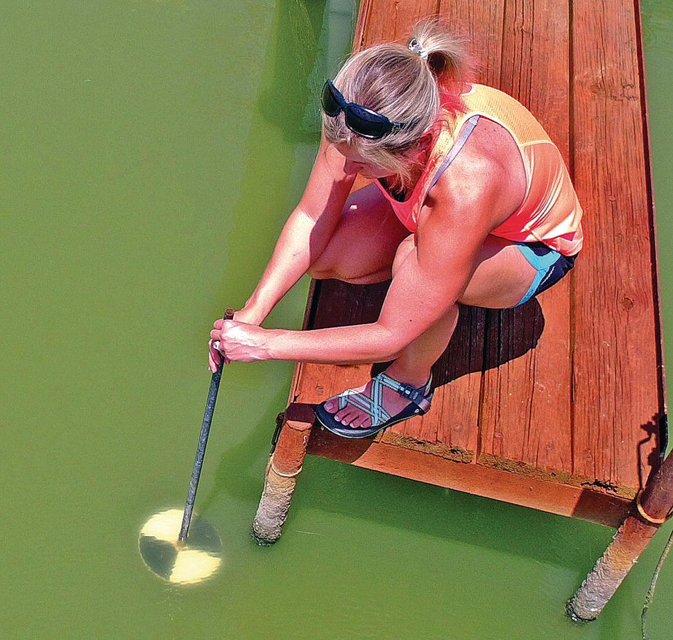
Figure 4.2 A Secchi disk is lowered into pond water to determine the turbidity. Using graduations on the rope (or handle), the turbidity is measured by noting the depth at which the disk is no longer visible.

Source: Reproduced with permission from Danny Oberle, 2017.

4.2.9 pH

The pH is the negative logarithm of the hydrogen ion concentration:

where (H⁺) = molar concentration of hydrogen ion. The pH concept originated in the ionisation of water:

The K_w is the equilibrium constant (K) for the dissociation of water. The value of K is a measure of the equilibrium position of a reaction. For the dissociation of water, K_w is very small (10⁻¹⁴), greatly favoring the reactant H₂O. Hydrogen ion concentration and pH of pure water are calculated as follows:

The pH concept allows hydrogen ion concentration to be expressed as a number between 0 and 14 rather than exponentially or as a small decimal fraction.

Hydrogen ion causes acidity, and pH expresses the degree of acidity. Pure water is neutral, neither basic nor acidic, because (H⁺) = (OH⁻). Waters with pH below 7 are acidic; those with pH above 7 are basic (or alkaline). Acidity increases as pH declines below 7 and declines as pH rises above 7. The opposite is true for basicity.

Because of the logarithmic nature of the pH, some argue that average pH values must be computed by first converting the pH values to hydrogen ion concentrations. These are averaged and then average pH is calculated from the average hydrogen ion concentration. This practice is almost always incorrect for aquaculture purposes and it is best to average pH measurements directly (Boyd et al. 2011).

4.2.10 Carbon Dioxide, Bicarbonate and Carbonate

Rainfall is naturally acidic because it is saturated with carbon dioxide (CO₂):

Carbon dioxide depresses the pH of rainwater to about 5.6. Lower rainfall pH values can be caused by sulphuric acid and other strong acids resulting from air pollution.

Acidity from carbon dioxide in rainwater dissolves limestone and silicate minerals¹:

Reaction of CO₂ with minerals is the source of bicarbonate (HCO₃⁻) in water. Bicarbonate does not occur at pH less than 4.5. At pH values between 4.5 and 8.3, water contains CO₂ and HCO₃⁻ and the proportions of these two substances establish the pH (Figure 4.3).

Figure 4.3 Mole fractions of dissolved inorganic carbon present as dissolved CO₂, HCO₃⁻ and CO₃²⁻ at different pH values.

Source: Reproduced with permission from Craig Tucker, 2017.

The CO₂ concentration is negligible at pH 8.3 and above, and HCO₃⁻ will be in equilibrium with carbonate (CO₃²⁻) instead of carbon dioxide:

The proportions of CO₂, HCO₃⁻ and CO₃²⁻ are related to pH (Figure 4.3) and, for practical purposes, only two of them coexist at a given pH. The two components form a buffer system to resist pH change. If H⁺ is added to water at pH 7.5, it will react with HCO₃⁻ to produce more CO₂, and pH will not change much as long as HCO₃⁻ is available. If OH⁻ is added to water of pH 7.5, it will react with CO₂ to produce more HCO₃⁻. This avoids a sharp rise in pH as long as CO₂ is present. No CO₂ is present at pH 8.3 and above, and HCO₃⁻ and CO₃²⁻ act as a buffer by reacting with added H⁺ and OH⁻.

Many submersed aquatic plants and most freshwater phytoplankton can use either CO₂ or HCO₃⁻ as a carbon source for photosynthesis. Plants that can use only dissolved CO₂ are generally restricted to waters with low HCO₃⁻ concentrations, because species that can use either CO₂ or HCO₃⁻ have a growth advantage in waters with abundant HCO₃⁻. Regardless of whether plants use CO₂, or HCO₃⁻ as a carbon source, the net effect of underwater photosynthesis is to increase water pH. When underwater respiration exceeds photosynthesis (at night, for example), excess CO₂ is produced and pH decreases. Reactions that are responsible for pH changes during photosynthesis and respiration are explained by Boyd et al. (2016).

4.2.11 Total Alkalinity and Total Hardness

• Total alkalinity is the acid‐neutralising capacity of water and includes all bases that are titrated with a strong acid to a pH of about 4.5.
• Total hardness is the concentration of all divalent cations in water; in most waters the major divalent cations are calcium and magnesium.

Total hardness can be measured by titration of divalent cations with the chelating agent ethylenediaminetetraacetic acid (EDTA) or by summing independent measurements of calcium and magnesium. Alkalinity and hardness are expressed in various ways depending on scientific discipline and country, but both are often expressed as equivalent CaCO₃. Concepts of alkalinity and hardness, their measurement and expression of concentration are explained in detail by Boyd et al. (2016).

Total alkalinity of natural water is seldom above 50 mg/L, as CaCO_3, in areas with acidic soils. Areas with neutral or basic soils, especially where soils contain limestone, usually have waters with 50–200 mg/L total alkalinity. Higher concentrations are often found in arid regions. Groundwater from limestone formations may contain up to 500 mg/L total alkalinity, but some groundwater may be very low in alkalinity. The average total alkalinity of seawater is 116 mg/L.

In humid areas, total hardness concentrations in water are normally similar to those of total alkalinity. Hardness may be considerably higher than total alkalinity in arid regions. Naturally softened groundwaters have lower hardness than alkalinity. The total hardness of seawater exceeds 6000 mg/L.

4.2.12 Nutrients

Plants require carbon, hydrogen, oxygen, nitrogen, sulphur, phosphorus, calcium, magnesium, potassium, sodium, iron, manganese, zinc, copper and possibly other elements. However, nitrogen and phosphorus are usually the two most important nutrients regulating plant productivity in aquatic ecosystems. Relatively large amounts of N and P may be added to aquaculture systems in fertilisers or feeds.

Phosphorus occurs in water primarily as phosphate ion (H₂PO₄⁻ or HPO₄²⁻) and in various organic compounds. In sediment, phosphorus forms poorly soluble compounds with iron and aluminium under acidic conditions and with calcium under basic conditions. The phosphorus concentration in water in equilibrium with sediment phosphorus is usually less than 10 µg/L. Most phosphorus in water is in plankton biomass or adsorbed on suspended soil particles. Total phosphorus concentrations are typically 10–20 times greater than concentrations of soluble phosphorus.

Nitrogen occurs in water in several forms: molecular nitrogen (N₂), ammonia (NH₃), ammonium (NH₄⁺), nitrite (NO₂⁻), nitrate (NO₃⁻) and organic nitrogen. Organic nitrogen may be dissolved or particulate, and particulate nitrogen may be in living organisms or in their remains.

The solubility of dinitrogen gas (N₂) in water is presented in Table 4.3. In unpolluted waters, concentrations of ammonia‐nitrogen and nitrate‐nitrogen seldom exceed 0.25 mg/L, and nitrite often is undetectable. Total nitrogen concentration may reach 1 mg/L. However, polluted water and water in aquaculture facilities may contain much greater concentrations of the various nitrogen compounds.

All aspects of the global nitrogen cycle (Figure 4.4) except fertiliser manufacture occur in lakes and ponds. Some bacteria and blue‐green algae can fix molecular nitrogen, and when they die and decompose, nitrogen is released as ammonia and enters the biological cycle. Rainfall contains nitrate because electrical activity in the atmosphere oxidises molecular nitrogen to nitrate. Ammonia is oxidised to nitrate by nitrifying bacteria in a two‐step process:

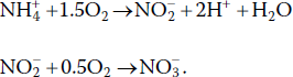
Figure 4.4 The global nitrogen cycle. Industrial fertiliser manufacture from atmospheric nitrogen gas is shown in red arrows.

Source: Reproduced with permission from Craig Tucker, 2017.

In anaerobic sediments and water, denitrifying bacteria reduce nitrate to molecular nitrogen as illustrated below using methanol as a carbon source:

Note the effects of nitrification and denitrification on pH: nitrification produces H⁺ and causes pH to decrease; denitrification produces OH⁻ and causes pH to increase. The effects of nitrogen transformations on pH can be important in aquaculture.

Plants use ammonium and nitrate for making amino acids and proteins. When plants die, their remains are decomposed by microorganisms with mineralisation of ammonia to the surrounding environment. Nitrogen is also contained in organic matter that accumulates in the bottoms of aquatic systems.

Both nitrogen and phosphorus are limiting factors for plant growth in most aquatic ecosystems including aquaculture systems. Excessive nitrogen and phosphorus concentrations in aquatic systems lead to eutrophication and undesirably dense phytoplankton blooms dominated by blue‐green algae.

4.2.13 Microorganisms and Water Quality

Phytoplankton abundance is controlled by availability of light and nutrients. In clear waters of low nutrient status, underwater weeds will flourish because they can obtain nutrients from sediments. Waters with a greater availability of waterborne nutrients will develop phytoplankton blooms unless humic substances or clay turbidity limit light availability.

Plants produce organic matter and release oxygen through photosynthesis:

Organic matter produced in photosynthesis is the base of the food web (Figure 4.5) in aquatic systems. All organisms respire and much of the oxygen produced in photosynthesis is used in respiration by the pond biota (including the phytoplankton and water weeds at night). Respiration, as an ecological process, is essentially the reverse of photosynthesis:

Figure 4.5 The food web of a shrimp pond.

Source: Reproduced with permission from Craig Tucker, 2017.

For our purposes, it is sufficient to note that plants produce organic matter that is either used in their respiration or in making their tissues. Plants become food for animals or substrate for organisms of decay. Phytoplankton remove nutrients from the water, while decomposer organisms recycle them.

Nitrifying and denitrifying bacteria have a major influence on ammonia and nitrate concentrations. High concentrations of nitrite result when the rate of ammonia oxidation to nitrite exceeds the rate of nitrite oxidation to nitrate. Nitrite can also accumulate when denitrifying bacteria produce nitrite instead of nitrogen gas under some conditions.

Dense phytoplankton blooms can cause shallow thermal stratification as cells absorb light and heat surface waters. Dead phytoplankton settles into the hypolimnion, causing DO depletion and the accumulation of potentially toxic microbial metabolites. Sudden destratification of water bodies resulting from high wind, heavy rains or other factors can mix hypolimnetic water with surface water, leading to DO depletion and fish kills.

In the afternoon, DO and pH will be higher in surface water than in deeper water while the opposite occurs with carbon dioxide. In water bodies that do not stratify thermally, oxygen depletion will not usually occur in bottom waters, but anaerobic zones may develop at the sediment‐water interface.

Phytoplankton affect DO, carbon dioxide concentrations and pH of water during the 24‐hr cycle of light and darkness. In daylight, photosynthesis uses carbon dioxide and produces DO faster than respiration releases carbon dioxide and uses oxygen. This results in an increase in DO concentration and a decrease in carbon dioxide concentration. The decrease in carbon dioxide causes pH to increase. At night, photosynthesis stops but respiration continues. Thus, DO declines and pH decreases because carbon dioxide concentration increases. The amount of fluctuation of the three variables increases as phytoplankton abundance increases. Depletion of DO may occur at night in water bodies with dense phytoplankton blooms (Figure 4.6). The likelihood of DO depletion increases during cloudy weather, because daytime DO concentration does not rise as high as usual and nighttime concentration will fall lower than normal.

Figure 4.6 Effect of time of day and plankton density on DO concentration in surface water of aquaculture ponds.

Source: Reproduced with permission from Craig Tucker, 2017.

Dense phytoplankton blooms may suddenly die because of exposure to excessive light or unexplained factors. Decomposition of the dead phytoplankton can result in DO depletion and fish kills.

4.2.14 Bottom Soils and Water Quality

Ponds with acidic bottom soils and filled with runoff water will be of low alkalinity and poorly buffered. Soils have a great affinity for phosphorus, and they control phosphorus concentrations and phytoplankton growth. Organic matter accumulates in pond bottoms, and bacteria degrade this material and recycle the nutrients in it. Bacterial activity uses oxygen faster than it can diffuse or infiltrate into pond bottoms. Below a depth of a few centimeters in oligotrophic water bodies or a few millimeters in eutrophic ones, sediment is anaerobic.

Organic matter is decomposed by fermentation under anaerobic conditions, but this process only partially degrades organic matter. Certain bacteria use oxygen from inorganic compounds in place of molecular oxygen to decompose organic matter completely to CO₂ and H₂O: denitrifying bacteria are an example. Other bacteria can use oxygen from iron and manganese compounds, sulphate and carbon dioxide in decomposing organic matter. These processes result in the release of nitrogen gas and nitrite, ferrous iron, manganous manganese, hydrogen sulphide and methane, respectively. Nitrite and hydrogen sulphide in particular are potentially toxic to aquatic animals. Other than methane and nitrogen gas, reduced substances do not normally diffuse into the water column because the sediment‐water interface tends to be aerobic.

Low pH in most soil results from the following reaction involving aluminium ions adsorbed to soil clay particles:

Liming material (as illustrated with CaCO₃) can be applied to the sediment to neutralise hydrogen ions:

Neutralisation of H⁺ results in release of aluminium ions from the soil to hydrolyze and precipitate as aluminium hydroxide, resulting in production of additional hydrogen ions that continue to be neutralised by calcium carbonate. A calcium ion from the reaction of CaCO₃ and H⁺ replaces Al³⁺ on the soil. This causes soil pH to increase. Enough calcium carbonate or other liming agent is applied to neutralise the acidity that can potentially result from exchangeable aluminium. Replacement of exchangeable aluminium with calcium will raise soil pH to near 7.

4.2.15 Feeding and Water Quality

Unmanaged waters, if unpolluted, may provide an excellent environment for fish but are usually unproductive because food is scarce. Food availability can be increased by using fertilisers to enhance natural productivity. Fertilisation is discussed later, in section 4.4.2. Aquaculture production from fertilised ponds depends on plant growth rate, which is eventually limited by the finite energy available from sunlight. To achieve greater production, food, usually in the form of manufactured feeds, must be imported from outside the culture system.

Only a portion of the feed applied is eaten. Fish quickly ingest feed pellets, and with careful feeding, 90% or more of the feed will be consumed. Shrimp nibble on feed pellets and 20–40% of feed may not be consumed directly. About 80 or 90% of the feed eaten by the farmed species is absorbed across the intestine and the remainder becomes faeces. Absorbed nutrients are used in metabolism and, to a lesser degree, for growth. Water, carbon dioxide, ammonia, phosphate and other compounds are excreted as metabolic wastes (Figure 4.7). A relatively small amount of the nutrients in the original feed input is captured in biomass of harvested animals. In one example, aquacultured shrimp contained only 12.2% of the carbon, 25.8% of the nitrogen and 14.2% of the phosphorus applied in feed. In fish culture, the percentages of feed carbon and nitrogen harvested in fish are similar to those for shrimp. However, unlike shrimp, fish have bones made of calcium phosphate and thus contain more phosphorus than shrimp. The percentage of feed phosphorus removed in fish at harvest is typically around 25–35%.

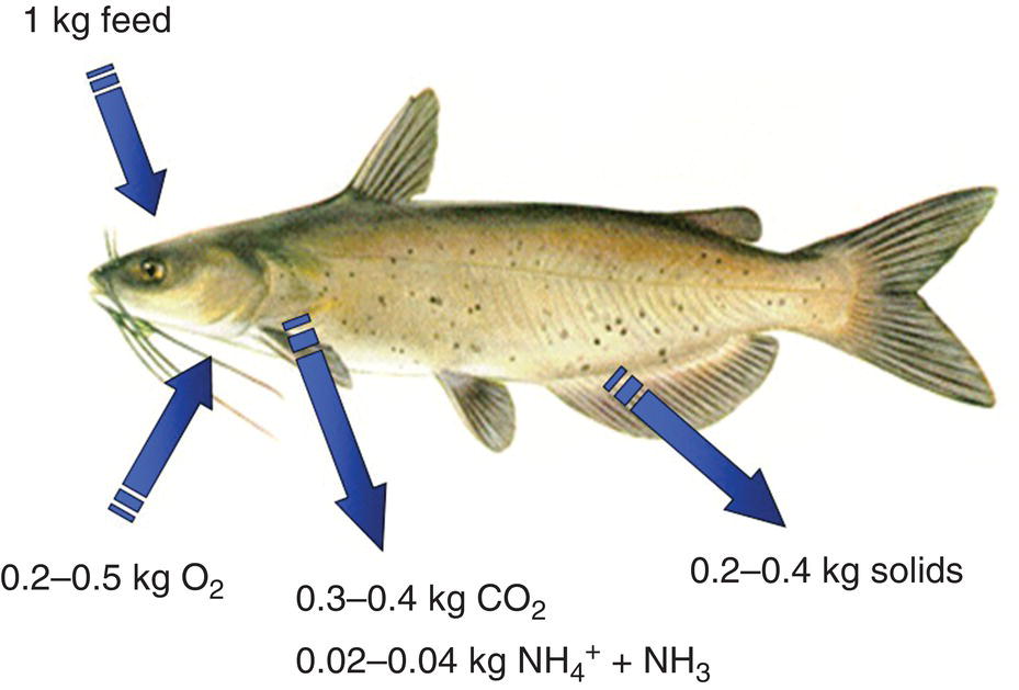
Figure 4.7 Waste production by fish as a result of feeding. Waste generation rates per kg of feed are typical values and will vary depending on fish species and size, food quality, feeding rate, water temperature and other factors.

Source: Reproduced with permission from Craig Tucker, 2017.

Wastes from feeding have a tremendous influence on pond water quality. In addition to ammonia, phosphate and other minerals excreted directly by animals, microorganisms decompose organic matter in uneaten feed and faeces, and release the same substances in the process called mineralisation. This decay process also removes DO from water and releases carbon dioxide.

Ammonia and phosphate stimulate growth of planktonic and benthic algae. Algal abundance in ponds increases as feed inputs increase. Ponds with dense blooms of planktonic algae typically have high DO concentrations during the day, but low DO at night can stress or kill the farmed species (Figure 4.6).

When daily feeding rates exceed 30–40 kg/ha, DO concentration will often fall to less than 3 or 4 mg/L at night. Low DO stresses cultured species, so mechanical aeration is necessary at higher daily feeding rates (section 4.4.3). Dissolved oxygen levels must be monitored, even in ponds with mechanical aeration, to avoid excessive feed input for the amount of aeration applied. Water exchange is sometimes used to flush plankton and nutrients from ponds and improve water quality. However, this practice can lead to water‐quality deterioration in receiving water bodies.

Ponds have a large capacity to assimilate wastes resulting from addition of feeds. As mentioned above, bacteria mineralise organic matter to carbon dioxide, ammonia and phosphate. Ammonia is lost to the atmosphere by volatilisation (diffusion). It is also oxidised to non‐toxic nitrate by nitrifying bacteria. Nitrate can be denitrified to nitrogen gas, which diffuses into the atmosphere. Carbon dioxide is converted to organic carbon by photosynthesis or diffuses from pond waters to the atmosphere. Bacteria can transform carbon dioxide in sediment to methane, which also diffuses to the atmosphere. Sediment usually has a large capacity to fix phosphorus in insoluble iron, aluminium and calcium phosphates. Some of the organic matter in ponds is relatively resistant to microbial decay and accumulates in sediment as stable organic matter. Although the waste‐treatment capacity of ponds is large, many ponds receive greater inputs of nutrients in feed than can be assimilated quickly, and water quality deteriorates. When this happens, the cultured species will be adversely affected and feed conversion efficiency will decline.

When ponds are drained for harvest, organic matter and nutrients in the water are discharged. The decomposition of new organic matter in pond bottoms can be hastened by allowing pond bottoms to dry and crack to facilitate aeration (Figure 22.9). By doing this each time a pond is drained, relatively low organic matter concentrations can be maintained indefinitely in pond bottoms. Of course, pond bottoms may eventually become saturated with phosphorus, which can lead to greater dissolved phosphorus concentrations and denser blooms of algae.

Feed inputs to ponds must not exceed the capacity of ponds to assimilate the resulting wastes. The most reliable way of determining how well a pond is assimilating wastes from feeding is to monitor early morning DO concentrations. Feeding and mechanical aeration rates must be adjusted to maintain DO concentrations above 3–4 mg/L in the early morning when the lowest concentrations occur.

4.3 Effects of Water Quality on Aquatic Animals

The effects of these water‐quality variables tend to follow three patterns (Figure 4.8). In Figure 4.8 ‘Performance’ includes factors such as level of feeding, growth, behaviour, survival, fecundity and immunity.

Figure 4.8 General responses of aquatic animals to increasing levels of environmental variables. (a) A distinct optimum level with decreasing performance at high and low levels. (b) Decreasing performance as levels increase. (c) Increasing performance as levels increase (although performance may decrease at very high level).

Source: Reproduced with permission from Craig Tucker, 2017.

4.3.1 Water Temperature

Temperature is perhaps the most important water‐quality variable because it directly or indirectly affects other water‐quality variables, natural productivity and culture species. Managing water temperature is economically unfeasible in outdoor aquaculture, and farmed species that grow well at the water temperature range of a particular site must be selected.

Increasing temperature increases the rate of physical processes, chemical reactions and metabolism and growth of organisms. Chemical reaction rates double with a 10 °C increase in temperature. This relationship applies to aquatic animal growth within their range of temperature tolerance. The factor of increase is called the Q₁₀, which is usually about 2 for aquatic animals. Of course, if temperature exceeds optimum, the growth of aquatic animals will decline.

Water temperature ranges for some common aquaculture species are provided in Table 4.4. This table gives the lower critical range, the range over which feeding occurs, the optimum range for growth and the upper critical range. To illustrate interpretation of data in the table, tilapia may die at water temperatures near 10 °C and 40 °C. They will not eat at temperatures below about 18 °C or above 35 °C. The best growth is achieved at temperatures of 28–32 °C.

Table 4.4 Critical water temperatures for six representative fish species.

Species	Lower critical1 range (°C)	Optimum2,3 range (°C)	Upper critical range (°C)
Oreochromis mossambicus (Java tilapia)	10–14	18‐(28‐32)‐35	36–42
Sciaenops ocellatus (red drum)	8–15	18‐(22‐28)‐30	34–40
Ictalurus punctatus (channel catfish)	0–10	15‐(25‐30)‐34	35–40
Micropterus salmoides (largemouth bass)	0–10	12‐(25‐30)‐32	32–38
Morone saxatilis (striped bass)	0–6	10‐(14‐24)‐28	30–34
Oncorhynchus mykiss (rainbow trout)	0–4	5‐(10‐16)‐20	22–26

¹ Upper and lower critical temperatures describe the ranges over which significant disturbances in metabolism may occur even if the fish are slowly acclimated to those temperatures. The more extreme value in the range is an approximation of the critical thermal maximum or minimum—the temperature at which only brief survival is expected.

² The optimum range is the temperature range over which feeding occurs.

³ Values in parentheses are the ranges for fastest growth.

The relationship between temperature and disease is complex because temperature affects host and pathogen. The immune system of aquatic animals functions best within the optimum temperature range for growth (Table 4.4). Sudden changes in temperature also impair the effectiveness of the immune system.

4.3.2 Salinity

Aquaculture species have a range of tolerance for salinity, for they must maintain a suitable salinity of internal fluids through osmoregulation or ion regulation. Freshwater fish and crustaceans have body fluids more concentrated in ions than the surrounding water; they are hypersaline or hypertonic to their environment. Saltwater species have body fluids more dilute than the surrounding water; they are hyposaline or hypotonic to their environment. Osmoregulation in freshwater fish involves the uptake of ions from the environment and restriction of ion loss. Freshwater fish tend to accumulate water because it is hypertonic to the environment, so it must excrete water and retain ions. On the other hand, osmoregulation for marine fish requires constant intake of water and excretion of ions. Because marine fish are hypotonic to the environment, they lose water. To replace this water, the fish takes in salt water; but to prevent the accumulation of excess salt, it must excrete salt.

Invertebrates such as decapod crustaceans and bivalves tend to conform to their environmental salinity more than fish. They tend to be isotonic in seawater, although the ion concentrations of their body fluids differ from seawater. Thus, they must regulate the uptake and loss of particular ions across their body surface. Crustaceans and especially bivalves living in freshwater or dilute brackishwater have lower body fluid concentrations than those in seawater. However, they are hypertonic to their environment and must regulate water and ions in the same manner as freshwater fish.

Each species has an optimum salinity range. Outside of this range the animal must expend considerable energy for osmoregulation at the expense of growth and other processes. If salinity deviates too much from the optimum, the animal will die because it cannot maintain internal salt balance.

Many freshwater fish can live in waters with salinities up to 5–10‰, but they may not reproduce or grow well at salinities above 3–4‰. Some species such as tilapia and rainbow trout can tolerate high salinity. Marine species are adapted to growth in ocean water and do not grow well at low salinity. Estuarine species are adapted to a wide range of salinity. Most species of farmed marine shrimp survive and grow well at salinities of 1–2‰ up to 35–40‰. Suboptimum salinity is especially stressful on aquaculture species when temperature also is outside the optimum range.

4.3.3 pH

The optimum pH for growth and health of most freshwater aquatic animals is in the range of 6.5 to 9.0. Acid and alkaline death points are approximately pH 4 and pH 11. Marine fish evolved in highly buffered seawater that is not subject to wide variation in pH. Consequently, most marine animals cannot tolerate as wide a range of environmental pH as freshwater animals, and the optimum pH is usually between pH 7.5 and 8.5. Some species evolved in estuaries where there is typically large variation in pH in response to variations in river discharge and tidal flow. Brackishwater inhabitants are rather tolerant of extremes of pH.

Gills are the primary target of elevated, environmental H⁺ concentration. For freshwater fish, changes in gill structure and function cause reduced ion uptake, increased ion loss, and reduced respiratory efficiency (Boyd and Tucker, 1998). Respiration is further compromised by blood acidosis, which decreases the affinity of haemoglobin for oxygen. Under mild acid stress, animals expend extra metabolic energy for maintenance of gill function at the expense of growth and immune function. Under extreme acid stress, the animal is not capable of maintaining homeostasis and dies.

Acid stress is most common in bodies of water where pH has declined because of human activities. For example, long‐term acidification of lakes because of acid precipitation has disastrous effects on natural fish populations in certain areas of Europe and North America. Low pH in aquaculture systems usually can be controlled through liming.

4.3.4 Dissolved Oxygen

Most of the oxygen carried in fish blood is associated with haemoglobin in red blood cells, although a small fraction dissolves in the plasma. Loading and unloading of haemoglobin with oxygen is governed by oxygen tension. At the gills, oxygen tension in water is higher than in the blood, and oxygen is loaded onto haemoglobin. In the tissues, oxygen is used rapidly and tissue fluids have a lower oxygen tension than blood entering the tissues from the arterial system. So, haemoglobin unloads oxygen to the tissue fluids. Invertebrates do not have haemoglobin in their blood. Most species contain another pigment, haemocyanin, which functions in much the same manner as haemoglobin.

In general, coldwater fish are more sensitive to hypoxia than are warmwater fish. Critical DO concentrations that negatively affect growth are lower than 5–6 mg/L for trout and salmon and 3–4 mg/L for warmwater fish.

As DO concentrations fall below critical levels, fish compensate for decreased availability of oxygen through behavioral and physiological changes. Ventilation volume increases because less oxygen is available in a given amount of water. Fish minimise extraneous activity to reduce metabolic oxygen demand. Certain physiological responses to low DO concentrations increase the capability for gas exchange at the gills. These adaptions and responses allow warmwater pond fish to survive for days even when DO concentrations are as low as 1–2 mg/L. At some point, compensatory responses are no longer sufficient and oxygen demand of tissues exceeds the amount that can be supplied. At about that point, fish swim to the surface in an attempt to exploit oxygen in the surface film. Eventually, the energy requirement for metabolism in the brain is not met and fish die. Adult warmwater fish can live for several hours at DO concentrations as low as 0.3–0.5 mg/L and fingerlings may survive short exposure to lower concentrations. Small fish consume more oxygen per unit weight than large fish because of their higher metabolic rate per unit weight. Small fish are also more effective at using oxygen in surface films than are large fish.

Coldwater fish usually die at a slightly higher oxygen concentration than required to kill warmwater fish. For example, rainbow trout may die at DO concentrations of 2.5–3.5 mg/L, and they do not grow well at DO concentration below 5 mg/L. Crustaceans are remarkably similar to fish in their tolerance to low DO concentrations.

Wide daily fluctuations in DO typically occur in intensive aquaculture ponds. In aquaculture ponds, DO concentrations often exceed 15 mg/L in the afternoon but fall below 5 mg/L by dawn. Usually, growth of most species decreases if DO concentrations before sunrise drop below 25% saturation. Of course, some aquaculture species such as tilapias and, especially, clariid and pangasiid catfishes are particularly tolerant to low DO concentrations. Concentrations of DO above saturation provide little benefit because the oxygen‐transporting pigment will fully load with oxygen when water is saturated with DO.

4.3.5 Carbon Dioxide

Aquatic animals excrete carbon dioxide produced in cellular respiration across their gills. When carbon dioxide concentration in water increases, the rate of excretion decreases leading to accumulation of blood carbon dioxide and a decrease in blood pH. These conditions decrease the affinity of respiratory pigments for oxygen, which reduces respiratory efficiency and decreases the tolerance of animals to low dissolved oxygen concentrations.

Tolerance of fish and crustaceans to environmental dissolved carbon dioxide concentrations varies greatly. Marine fish evolved in environments with stable, low dissolved carbon dioxide concentrations and are intolerant of dissolved carbon dioxide. Long‐term exposure to more than 5 mg/L may reduce growth. An upper limit of 20 mg/L dissolved carbon dioxide has been suggested for the health of salmonids. Warmwater fish evolved in environments where fluctuations in dissolved carbon are more common and, therefore, can tolerate higher concentrations. Concentrations of dissolved carbon dioxide greater than 60 to 80 mg/L have a narcotic effect on aquatic animals and even higher concentrations may cause death.

Most studies have concentrated on the effects of long‐term exposure to specific carbon dioxide concentrations. Such information has application to culture systems where carbon dioxide concentration is relatively stable over time. Carbon dioxide concentrations in ponds may change by an order of magnitude between night and day. No studies have been made of the effects of short‐term exposure of fish or crustaceans to fluctuating carbon dioxide concentrations so it is difficult to assess the overall importance of carbon dioxide to pond aquaculture.

4.3.6 Gas Supersaturation

Water can become supersaturated with gases by several processes: rapid increase in temperature; mixing of air‐saturated water masses of different temperatures; expulsion of air into surrounding water during ice formation; air entrainment by falling water; leaks on suction side of pumps; submerged aerators; photosynthesis (oxygen only); or sudden changes in barometric pressure. Gas supersaturation is expressed as the ΔP value which is calculated by subtracting local barometric pressure from total gas pressure in the water or by measuring it directly with a saturometer.

Supersaturation is an unstable condition and as gases come out of solution they form bubbles. If the dissolved gases diffuse across the gill before coming out of solution, emboli will form in the vascular system and other tissues: a condition called gas bubble disease. Acute gas bubble disease occurs at high levels of supersaturation, usually at ΔP values of about 15 kPa or greater. Eggs will float to the surface, and larvae and fry may exhibit hyperinflation of the swim bladder, exophthalmos (‘pop‐eye’), cranial swelling, swollen gills, blood in the abdominal cavity, gas bubbles in yolk sac and distention and rupture of yolk sac membrane. In juvenile and adult fish, the most common symptoms of acute gas bubble disease are gas bubbles in the blood and bubble formation in gill filaments, on the head, in the mouth and in fin rays. The eyes will also protrude. Mortality rates can be high and death is caused by bubbles that restrict blood flow. When aquatic animals are exposed to ΔP values of 5–15 kPa on a continuous basis, chronic gas bubble disease may develop. Symptoms are bubble formation in gut and mouth, hyperinflation of the swim bladder and low‐level mortality. Death is often caused by secondary, stress‐related infections.

Although animals may potentially develop gas bubble disease any time there is a positive ΔP, occurrence is strongly influenced by the depth at which animals spend most of their time. Higher hydrostatic pressure at depth means that a larger gas concentration is necessary for supersaturation. Water depth can also affect the potential for developing gas bubble trauma because rates of photosynthesis and solar heating decrease with depth.

Despite the frequent occurrence of supersaturated conditions in surface waters, gas bubble trauma rarely occurs in aquaculture ponds. Apparently, if supersaturation of surface water reaches harmful levels in ponds, animals will move into deeper waters where ΔP is lower. In most ponds, supersaturation will only threaten eggs or fry restricted to the surface by lack of mobility. In shallow ponds with clear water and abundant submersed vegetation, the entire water volume can become strongly supersaturated and there is no refuge for animals.

4.3.7 Ammonia and Nitrite

Ammonia exists in two forms, un‐ionised ammonia (NH₃) and ammonium ion (NH₄⁺), in a pH‐ and temperature‐dependent equilibrium:

As pH rises, NH₃ increases relative to NH₄⁺. Water temperature also causes an increase in the proportion of un‐ionised ammonia, but the effect of temperature is less than that of pH. The common analytical procedures for ammonia measure total ammonia‐nitrogen (TAN) which includes both NH₃‐N and NH₄⁺‐N. Decimal fractions of TAN concentrations occurring as NH₃‐N at different temperature and pH values (Table 4.5) may be used to estimate NH₃‐N from TAN.

Table 4.5 Decimal fractions of total ammonia‐nitrogen existing as un‐ionised ammonia‐nitrogen at various pH values and water temperatures. Values were calculated using the ‘ammonia calculator’ at http://fisheries.org/hatchery for a typical, dilute fresh water with a TDS concentration of 250 mg/L.

Source: Adapted from Boyd and Tucker (2014).

	Temperature (°C)
pH	5	10	15	20	25	30	35
7.0	0.001	0.002	0.003	0.004	0.005	0.007	0.010
7.5	0.004	0.005	0.008	0.011	0.016	0.023	0.032
8.0	0.011	0.017	0.024	0.035	0.050	0.069	0.093
8.5	0.035	0.051	0.073	0.103	0.141	0.189	0.246
9.0	0.103	0.146	0.200	0.267	0.342	0.424	0.507
9.5	0.266	0.350	0.442	0.535	0.622	0.699	0.765
10.0	0.534	0.630	0.715	0.784	0.839	0.880	0.911

‘Ammonia toxicity’ to fish and other aquatic creatures is attributed primarily to NH₃. As ammonia concentration in water increases, ammonia excretion by aquatic organisms diminishes, and levels of ammonia in blood and other tissues increase. The result is an elevation in blood pH and adverse effects on enzyme‐catalyzed reactions and membrane stability. Ammonia increases oxygen consumption by tissues, damages gills and reduces the ability of blood to transport oxygen. Its toxicity is usually expressed by reduced growth rate instead of mortality. However, disease susceptibility also increases in organisms exposed to sub‐lethal concentrations of ammonia. Tolerance to ammonia varies with species, physiological condition and environmental factors. Lethal concentrations to warmwater fish and crustaceans for 24–96 hr exposure are between 0.4 and 2.0 mg/L NH₃‐N.

Risk of ammonia intoxication is difficult to evaluate for pond‐grown animals because daily fluctuation in pH causes NH₃ concentrations to change continuously. Although afternoon pH (and, therefore, NH₃ levels) may be high in ponds, it seldom remains at its greatest level for more than a few hours. When pH declines at night, NH₃ concentrations decrease and ammonia that may have accumulated in the blood during daylight, when pH was high, can then be excreted across the gills.

Nitrite may accumulate to concentrations of 1–10 mg/L NO₂⁻‐N, or more, in water of aquaculture systems under certain conditions. When nitrite is absorbed by fish, it oxidises ferrous iron in haemoglobin to ferric iron to form methaemoglobin that is not capable of combining with oxygen. Blood containing significant amounts of methaemoglobin is brown, so nitrite poisoning is commonly called ‘brown blood disease.’ Crustaceans contain haemocyanin, a compound similar to haemoglobin but with copper instead of iron. Reactions of nitrite with haemocyanin are poorly understood, but nitrite can be toxic to crustaceans.

Tolerance to nitrite varies greatly. Tilapia, carp, catfish, and trout and salmon are sensitive because nitrite is concentrated into the blood by the same gill anion‐uptake mechanism responsible for uptake of chloride. Freshwater sunfishes (Centrarchidae), temperate basses (Moronidae), and perhaps others exclude nitrite from the bloodstream and these fish are relatively tolerant. Marine fish are also tolerant of nitrite because of the high chloride concentration in seawater.

Because chloride and nitrite are concentrated by the same mechanism in nitrite‐sensitive species, the amount of nitrite entering the blood (and thus the amount of methaemoglobin formed) depends on the ratio of chloride to nitrite in the water. Either raising the chloride concentration or lowering the nitrite concentration will decrease nitrite uptake by competitive exclusion of ion uptake. The simplest procedure for counteracting nitrite toxicity in fish is to treat water with common salt (NaCl) to increase reduce the ratio of chloride to nitrite. A Cl: NO₂⁻‐N ratio of 20:1 prevents negative effects of high NO₂⁻‐N concentration on channel catfish and seems to have broad application to other nitrite‐sensitive species. Water exchange or replacement also can be effective in reducing NO₂⁻‐N concentrations.

Determination of the highest permissible NO₂‐N concentration for pond waters is difficult because of interactions with chloride and because nitrite toxicity is closely related to DO concentrations. Generally, pond managers should be concerned when NO₂⁻‐N concentrations exceed 2 or 3 mg/L.

4.3.8 Hydrogen Sulphide

Sulphide is an ionisation product of hydrogen sulphide and participates in the following equilibria:

The pH regulates the distribution of total sulphide among its forms (H₂S, HS⁻ and S²⁻). Un‐ionised hydrogen sulphide (H₂S) is toxic to aquatic organisms; the ionic forms have no appreciable toxicity. Analytical procedures measure total sulphide. The proportions (decimal fractions) of total sulphide‐sulphur occurring as un‐ionised hydrogen sulphide at different pH values at 28 °C are presented in Table 4.6. The proportion of hydrogen sulphide decreases as the pH increases. These decimal fractions may be multiplied by total sulphide‐sulphur concentrations to give the hydrogen sulphide concentration (as sulphur).

Table 4.6 Decimal fractions (proportions) of total sulphide‐sulphur existing as un‐ionised hydrogen sulfide in freshwater at different pH values and temperatures. Note: multiply values by 0.9 for seawater.

Source: Adapted from Boyd and Tucker (2014).

	Temperature
pH	16	18	20	22	24	26	28	30	32
5.0	0.993	0.992	0.992	0.991	0.991	0.990	0.989	0.989	0.989
5.5	0.977	0.976	0.974	0.973	0.971	0.969	0.967	0.965	0.963
6.0	0.932	0.928	0.923	0.920	0.914	0.908	0.903	0.897	0.891
6.5	0.812	0.802	0.792	0.781	0.770	0.758	0.746	0.734	0.721
7.0	0.577	0.562	0.546	0.530	0.514	0.497	0.482	0.466	0.450
7.5	0.301	0.289	0.275	0.263	0.250	0.238	0.227	0.216	0.206
8.0	0.120	0.114	0.107	0.101	0.096	0.090	0.085	0.080	0.076
8.5	0.041	0.039	0.037	0.034	0.032	0.030	0.029	0.027	0.025
9.0	0.013	0.013	0.012	0.011	0.010	0.010	0.009	0.009	0.008

Concentrations of 0.01–0.05 mg/L of hydrogen sulphide may be lethal to aquatic organisms. Any detectable hydrogen sulphide is considered undesirable. The presence of hydrogen sulphide may be recognised without water analysis, for the ‘rotten‐egg’ smell of hydrogen sulphide is detectable at very low concentration.

4.3.9 Total Alkalinity and Total Hardness

Total alkalinity results primarily from bicarbonate in waters for aquaculture, and fish have no direct requirement for bicarbonate. There is evidence that crustaceans need bicarbonate when molting, and 50–100 mg/L is considered sufficient for this purpose. Waters with low total alkalinity are poorly buffered and the availability of carbon for photosynthesis is limited. Waters containing 50 mg/L or more total alkalinity have more stable water quality and are more productive than waters of lower total alkalinity. Waters with total alkalinity more than 200–300 mg/L may have high pH and low availability of phosphorus.

Groundwater from some aquifers is both supersaturated with carbon dioxide and high in total alkalinity. When such water is exposed to the air, carbon dioxide is lost, and a portion of the bicarbonate is transformed to carbonate and precipitates as calcium carbonate. This phenomenon is usually not harmful in ponds or other large grow‐out units, but precipitation of calcium carbonate on eggs or fry of fish or shrimp in hatcheries may be harmful.

In freshwater aquaculture systems, total hardness concentration will usually be similar to that of total alkalinity. The most common aberration involves certain well waters with hardnesses drastically lower than alkalinities. When used in ponds, such water may develop very high pH in response to photosynthesis. In brackishwater and seawater, total hardness will be many times greater than total alkalinity. This condition does not cause problems with culture species.

Calcium is a major contributor to total hardness in freshwater, and low hardness is an indicator of low calcium concentration. Adequate calcium in water is essential for good hatchability of fish eggs. In seawater, magnesium contributes much more to hardness than does calcium.

Boyd et al. (2016) provide a detailed summary of alkalinity and hardness and their management in aquaculture.

4.4 Pond Water‐Quality Management

Aquaculture water‐quality management usually has one of four goals:

1. Correcting problems with the facility’s water supply.
2. Enhancing the productivity of ponds that rely on in‐pond primary productivity to support aquaculture production.
3. Mitigating the negative consequences of using manufactured feeds to support aquaculture production.
4. Reducing the impact of aquacultural effluents on receiving water bodies.

Technologies exist for correcting any water‐quality problem associated with source waters, but it is almost always too costly to attempt treatment except for small facilities or facilities raising high‐value animals. Problems with water supplies are best addressed by carefully selecting sites with water of adequate volume and proper quality.

The remainder of this chapter will focus on some common water‐quality management practices, with emphasis on enhancing pond productivity and preventing water‐quality deterioration in ponds with feeding. Emphasis on pond aquaculture is justified because ponds are far and away the most common aquaculture system in the world. Water‐quality management in other systems is briefly discussed in section 4.4.11. Additional information on water‐quality management in ponds and other aquaculture systems is found in Boyd and Tucker (1998, 2014) and Tidwell (2012). Treating aquacultural effluents is discussed later, in section 4.5.

4.4.1 Liming of Acidic, Low‐Alkalinity Pond Waters

Ponds built on sulphidic soils, often called acid‐sulphate soils, may have waters with pH values so low that culture species will not survive, or if they survive, they will not grow well. Such situations may be corrected by heavy liming and management procedures designed to minimise the contact of sulphide‐bearing soil with the air to prevent its oxidation and the formation of sulphuric acid. However, it is best to avoid using sites with potential acid‐sulphate soils for aquaculture.

The more common acidity problem occurs in ponds constructed on soils with a high concentration of exchangeable aluminium. Waters in such ponds have pH of 5.5–6.5 and alkalinity below 20 mg/L. Fish will grow in such waters, but natural productivity of fish food organisms will be low, and waters will be poorly buffered against pH change in response to phytoplankton photosynthesis. Liming materials increase the pH of bottom soils and elevate alkalinity and hardness in water. These changes improve conditions for microbial activity and growth of benthic animals; increase the availability of carbon dioxide, phosphorus and other nutrients; enhance phytoplankton growth; and improve the survival and growth of the aquacultural crop.

The most common liming materials are agricultural limestone, burnt lime and hydrated lime. These products are made from limestone, which is a relatively soft rock composed of calcium carbonate (CaCO₃ or calcite), calcium magnesium carbonate (CaCO₃.MgCO₃ or dolomite) or a mixture of these carbonates. Burnt lime, CaO, is made by burning limestone in a furnace at high temperature. Hydrated lime, Ca(OH)₂, is made by treating burnt lime with water. Both burnt lime and hydrated lime are usually fine white powders.

Agricultural limestone is the safest and least expensive liming agent to use for routine management of ponds with low alkalinity and acidic bottom soils. Agricultural limestone dissolves slowly and does not cause rapid changes in water pH. Burnt lime and hydrated lime have the same overall effects as agricultural limestone, but initially cause a much higher pH and are not normally applied to pond water during the culture period. These two materials, however, can be applied to the bottoms of empty ponds at 2000–3000 kg/ha to raise pH and kill pathogens and other unwanted organisms. Hydrated lime reacts with carbon dioxide and is sometimes used as a treatment for high carbon dioxide levels.

Ponds with total alkalinity below 50–60 mg/L must be limed. The liming rate needed to increase soil pH and total alkalinity can be estimated by one of several lime requirement tests which are described elsewhere (Boyd and Tucker, 2014). An alternative is to measure pond soil pH in a 1:1 mixture of dry pulverised pond soil and distilled water. The liming rate can be selected based on bottom soil pH from Table 4.7. Another approach is to apply agricultural limestone at 1,000 kg/ha and check total alkalinity after 3–4 wk. If the alkalinity is still low, more agricultural limestone may be applied.

Table 4.7 Lime requirements (kg/ha) based on soil pH and soil texture.

	Soil texture
SoilpH	Clayey	Loamy	Sandy
<4.5	5,000	4,000	2,500
4.5–5.0	4,000	3,000	2,000
5.1–5.5	3,000	2,000	1,500
5.6–6.0	2,000	1,500	1,000
6.1–6.5	1,500	1,000	750
6.6–7.0	1,000	750	500
7.1–7.5	500	375	250
>7.5	0	0	0

Application of agricultural limestone to water normally increases total alkalinity and hardness by roughly equal amounts. The solubility of calcium carbonate in water in equilibrium with normal atmospheric concentrations of carbon dioxide is about 60 mg/L. In ponds, there is usually more carbon dioxide available from organic matter decomposition and more calcium carbonate is dissolved. Nevertheless, if pond waters contain more than 80–100 mg/L alkalinity, agricultural limestone will not usually dissolve.

It is important that agricultural limestone be spread over the entire pond. This can best be done when ponds are empty between crops, but limestone may also be spread over the pond surface from a boat. Acidic ponds will usually need to be limed after every crop if they are drained for harvest. Acidic ponds that are not drained for harvest usually need to be limed at 3‐ to 4‐yr intervals.

4.4.2 Pond Fertilisation

Fertilisers are frequently used in pond aquaculture to stimulate phytoplankton productivity and enhance the availability of natural food organisms. Turbidity created by phytoplankton also shades pond bottoms to discourage the growth of underwater aquatic weeds. Ponds may be fertilised with organic materials such as animal excrement, agricultural byproducts, or grass. They may also be fertilised with chemical fertilisers.

4.4.2.1 Organic Fertilisers

Organic fertilisers, sometimes called ‘manures’ usually consist of relatively low‐quality substances that might otherwise be considered a waste product, such as poultry manure, poultry litter, cowshed manure, plant byproducts and wastewater. Organic material added to ponds provides food for animals in three ways, although in practice all three contribute to growth of the animal under culture.

First, POM may be consumed directly by animals. This is usually a minor contribution because most organic fertilisers are nutritionally inadequate, unpalatable or too difficult to ingest to support high food animal production through direct consumption.

Second, the organic material is partially decomposed by bacteria and fungi resulting in the production of high‐quality detritus consisting of microbial biomass and partially decomposed organic matter. The detritus is consumed by zooplankton and benthic macroinvertebrates. The detritus, as well as the zooplankton and macroinvertebrate consumers, are then eaten by the animal under culture.

The third food pathway originates when inorganic nutrients (nitrogen, phosphorus and others) and carbon dioxide are released as the organic matter decomposes. These nutrients stimulate plant growth, which then serves as the base of complex food webs culminating in growth of the animal under culture.

Organic fertilisers have their maximum benefit in developing countries where small‐scale farmers may have low‐quality materials available from farm livestock and cannot afford chemical fertilisers. Although it seems to be an unsophisticated practice, fish production in organically fertilised ponds can be as high as or higher than that achieved with chemical fertilisers. There are, however, several disadvantages to manures:

• most organic fertilisers have a low percentage of nutrients and vary in composition;
• because of low nutrient quality, large application rates are necessary;
• large applications can cause DO depletion and accumulation of partially decomposed manure in pond bottoms: application rates should not exceed about 50 kg/ha of dry matter per day in un‐aerated ponds to avoid DO depression by microbial degradation of the material;
• organic fertilisers encourage growth of algal mats;
• organic fertilisers may contain antibiotics put into animal feeds, and they have high concentrations of trace metals; and
• many consumers have negative attitudes about aquaculture products from organically fertilised ponds.

4.4.2.2 Chemical Fertilisers

The concept behind chemical fertilisation is that key plant nutrients are added to the pond to stimulate plant growth (primary production) which, in turn, serves as the base of food webs that ultimately culminate in the growth of the animal under culture. Key nutrients for aquatic plant growth are phosphorous and nitrogen. Potassium and other nutrients are sometimes important.

The two most common fertilisers used worldwide in aquaculture are triple superphosphate and urea. Other common fertilisers used in aquaculture are listed in Table 4.8. Most fertilisers are packed in bags and sold as dry granules or prills (spherical pellets), but ammonium polyphosphate and phosphoric acid are liquids.

Table 4.8 Approximate grades of common commercial fertilisers.

	Percentage
Fertiliser	N	P2O5	K2O
Urea	45	0	0
Calcium nitrate	15	0	0
Sodium nitrate	16	0	0
Ammonium nitrate	33–35	0	0
Ammonium sulphate	20–21	0	0
Superphosphate	0	18–20	0
Triple superphosphate	0	44–54	0
Monoammonium phosphate	11	48	0
Diammonium phosphate	18	48	0
Calcium metaphosphate	0	62–64	0
Potassium nitrate	13	0	44
Potassium sulphate	0	0	50
Potassium chloride (muriate of potash)	0	0	60

Nitrogen is usually added as urea, ammonium or nitrate. Phosphorus occurs as orthophosphate or polyphosphate, while potassium is in its ionic form. Fertilisers dissolve in water to release their nutrients. Urea begins to hydrolyze at once and is completely transformed to ammonia and carbon dioxide within a few days. Polyphosphate also quickly hydrolyzes to orthophosphate.

The grade of a fertiliser is usually reported as percentages of nitrogen (N), phosphorus oxide (P₂O₅), and potassium oxide (K₂O). Thus, triple superphosphate is usually a 0‐46‐0 fertiliser, diammonium phosphate is a 18‐48‐0 fertiliser and urea is a 45‐0‐0 fertiliser. Table 4.9 shows the approximate grades of common commercial fertilisers. Note that some primary fertiliser sources contain one primary nutrient, such as urea or triple superphosphate, while others may contain two primary nutrients such as diammonium phosphate and potassium phosphate. A mixed fertiliser is made by blending two or more primary fertiliser sources to provide two or three primary nutrients. Mixed fertilisers representing a wide range of grades can be purchased in most countries.

Table 4.9 Nitrogen and phosphorus budgets as percentages of the original input of the two elements in feed to catfish ponds.

Pathway	Nitrogen	Phosphorus
Harvest in fish	31.5	31.0
Ammonia volatilisation	12.5	—
Denitrification	17.4	—
Sediment accumulation	22.6	57.6
Effluent	16.0	11.4

Sometimes, fertilisers will be supplemented with the secondary nutrients calcium, magnesium and sulphur. The usual sources of these elements are calcium and magnesium sulphates. Supplements of trace elements, iron, manganese, zinc, copper, boron and others may be added to fertilisers.

Fertiliser granules or prills are water soluble but settle to the pond bottom before completely dissolving. Much of the phosphorus may be adsorbed by the bottom soil instead of remaining in the water. This problem can be lessened by using liquid fertilisers.

Liquid fertilisers are denser than water and must be diluted 1:10 with pond water and splashed over pond surfaces or released into the propeller wash of an outboard motor while a boat is driven over the pond surface. If liquid fertilisers are not available or considered too expensive, granular or prilled fertilisers may be placed in 10 to 20 times their volume of pond water, pre‐dissolved by vigorous stirring and splashed over the water surface.

Typical application rates of N and P₂O₅ are 2–10 kg/ha each per application. Many farmers apply excessive nitrogen. We recommend applications of 2 kg N/ha and 8 kg P₂O₅/ha for freshwater ponds and 8 kg/ha each for N and P₂O₅ for ponds filled with brackishwater or seawater.

Diammonium phosphate or monoammonium phosphate are good fertilisers for freshwater, because they have N:P₂O₅ ratios of about 1:3 and 1:4, respectively. For brackishwater or seawater, a fertiliser with a N:P₂O₅ ratio of 1:1 is best, and a mixed fertiliser with a 20‐20‐0 grade is a good choice. In brackishwater ponds for shrimp culture, many farmers want to encourage diatom growth. This can be done by applying nitrogen fertilisers weekly at 2–3 kg N/ha. Nitrate is especially efficient in promoting diatoms and sodium nitrate can be used as a diatom‐promoting fertiliser.

Fertiliser may need to be applied at intervals of 2‐ to 4‐wk to maintain phytoplankton blooms. However, more frequent applications may be necessary to initiate blooms. In ponds with feed applications, nutrients enter the water from feed wastes and applications of fertilisers often are unnecessary or only necessary until feeding rates reach 15 or 20 kg/ha per day.

Once blooms have been initiated, fertiliser can be applied according to need as judged from the Secchi disk visibility. A Secchi disk visibility of 25–40 cm is usually considered adequate. As an example, where the normal application rate is 2 kg N/ha and 8 kg P₂O₅/ha, the application rate might be adjusted for Secchi disk (SD) visibility as follows: SD ≤25 cm, 0 kg N and P₂O₅; SD = 26–30 cm, 0.5 kg N and 2 kg P₂O₅/ha; SD = 31–35 cm, 1 kg N and 4 kg P₂O₅/ha; SD = 36–40 cm, 1.5 kg N and 6 kg P₂O₅/ha; SD >40 cm, 2 kg N and 8 kg P₂O₅/ha.

Fertilisers containing ammonium or urea are potentially acidic because nitrifying bacteria in water can oxidise ammonia to nitrate and yield hydrogen ion. The hydrogen ion will react in water to decrease total alkalinity and pH. The adverse influence of nitrification on alkalinity and pH can be counteracted by routine applications of agricultural limestone to ponds where alkalinity is naturally low. In brackishwater, seawater and freshwater with alkalinity above 50 mg/L, acidity from nitrogen fertilisers is not a problem.

4.4.3 Mechanical Aeration and Mixing

Mechanical aeration is used widely in pond aquaculture to prevent low DO concentrations, especially at night; improve the efficiency of feed use; and increase fish or shrimp production. Mechanical aerators increase the rate of oxygen transfer from air by providing a greater surface area between air and water. This is achieved by splashing water into air or by releasing bubbles into water.

Aerators are most effective when DO concentrations in water are low, because the driving force causing oxygen to enter the water is the difference in pressure between oxygen in air and oxygen in water. Likewise, aerators transfer oxygen from water to air when water is supersaturated with DO.

In addition to transferring oxygen to water, aerators circulate pond water. Water circulation is beneficial in moving oxygenated water away from aerators to prevent localised saturation and loss of oxygen‐transfer efficiency by the aerator. It also prevents ponds from thermally stratifying. Aerator‐induced water currents transport oxygen throughout the pond for use by the culture species. Circulation creates ripples on the water surface that favor the outward diffusion of ammonia and other toxic gases. It also delivers water containing DO over the pond bottoms to avoid localised pockets of anaerobic sediment.

In ponds with a high animal biomass, aeration may be necessary during daytime to provide circulation even though little or no oxygen transfer results. However, the amount of aeration applied must be reduced during daytime to minimise oxygen loss to the air and lessen energy costs. At night, aeration must be increased to prevent low DO concentration.

There are many kinds of mechanical aerators. Paddlewheel aerators and vertical turbine aerators (Figures 4.9 and 4.10) are two common types of aerators. Diffused‐air aeration systems release bubbles of air near pond bottoms to rise through the water column. Another type is the propeller‐aspirator‐pump aerator, which releases tiny air bubbles into turbulent water created by a rapidly rotating impeller.

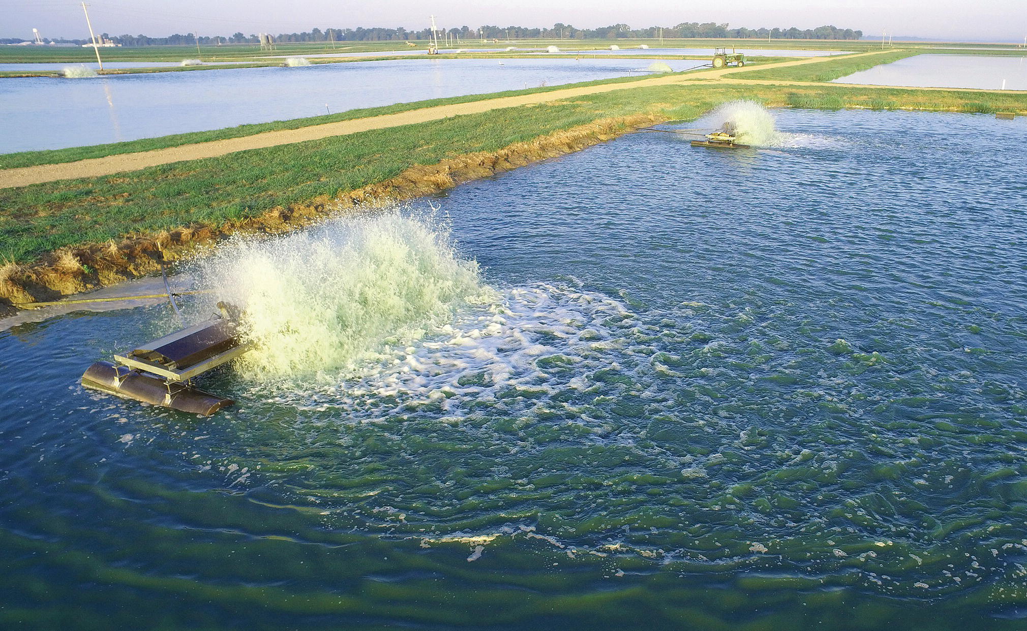
Figure 4.9 Paddlewheel aerators in a catfish pond.

Source: Reproduced with permission from Danny Oberle, 2017.

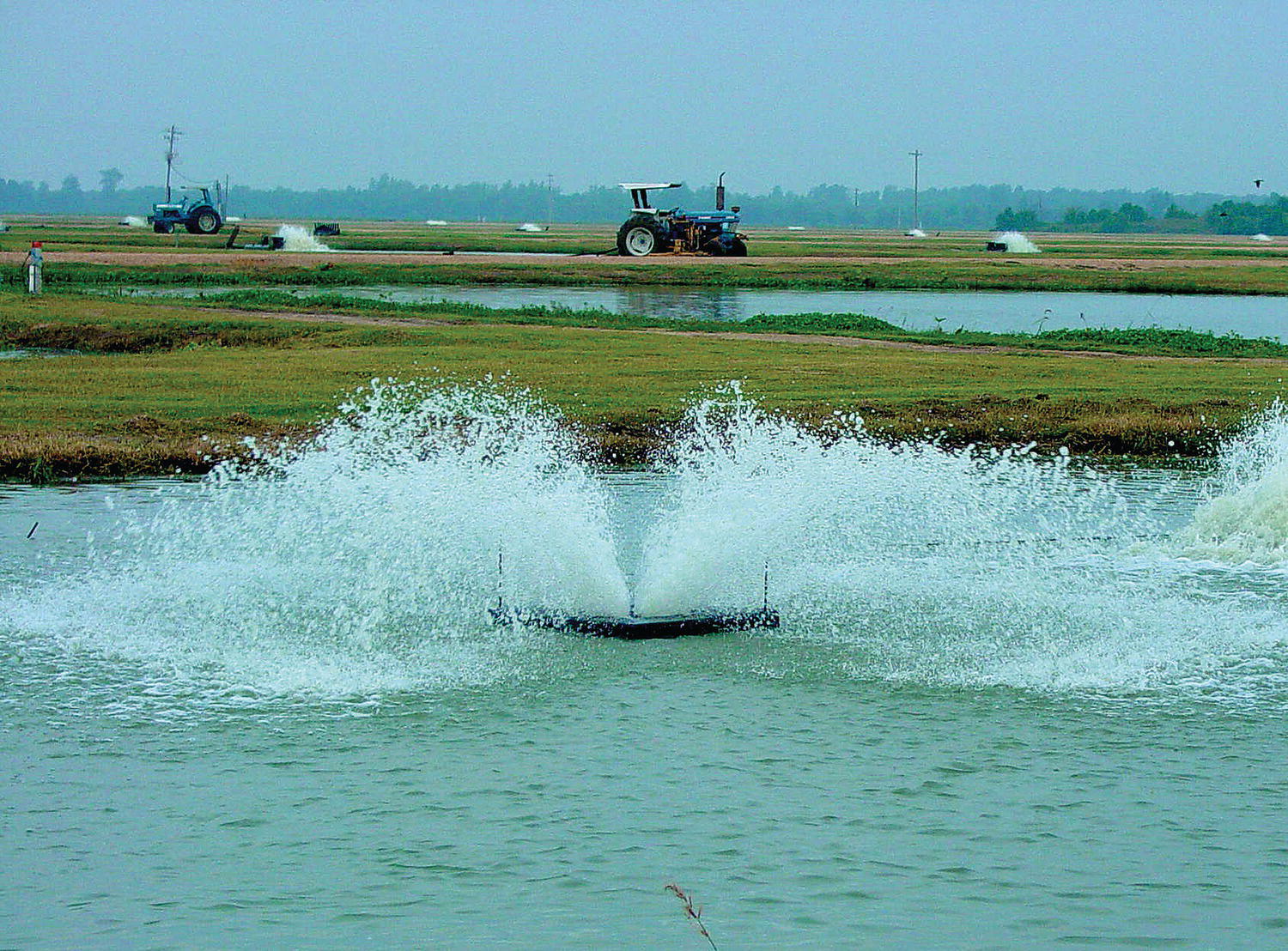
Figure 4.10 A vertical‐pump (sprayer‐type) aerator.

Source: Reproduced with permission from Les Torrans, 2017.

The standard aeration efficiency (SAE) is the quantity of oxygen an aerator will transfer per kilowatt of power in 1 hr when standardised to conditions of 20 °C, 0 mg/L DO, and clean water. Typical SAE values range from 1 to 2 kg oxygen/kW per hr. Oxygen‐transfer rate decreases as ambient DO concentrations increase above 0 mg/L; during operation in a pond containing 3–4 mg/L DO, the actual oxygen‐transfer rate will be 40–50% of the SAE.

Experience and calculations based on pond oxygen budgets suggest that production can be increased by about 500 kg for each kW of aeration applied. For example, suppose 1500 kg/ha can be produced without mechanical aeration. To increase production by 3500 kg/ha to 5000 kg/ha, the minimum aeration requirement will be about 7 kW/ha (3500 kg/ha ÷ 500 kg/kW). However, to reduce risks, a safety factor of 1.5 must be applied, resulting in an aeration requirement of about 11 kW/ha in our example.

Few studies have examined the best ways of positioning aerators in ponds. Fish move to aerated zones, so positioning is less important in fish ponds than in shrimp ponds. In fact, in channel catfish farming, all aerators are located in one end of the pond, near the source of electrical power. This practice allows the use of a single electrical service panel and greatly reduces the amount of electrical wire between the panel and aerators.

In shrimp ponds, the long‐standing practice of positioning aerators to create a circular movement of water is probably as good as any other alternative. To avoid erosion, aerators must not be mounted in water less than 0.75‐m deep or near embankments. Water currents also must not impinge on embankments for the same reason. Moreover, water currents from one aerator must not collide with currents from another.

Oxygen production in photosynthesis occurs in surface waters and if waters are thermally stratified, oxygen cannot be distributed to bottom waters. Mechanical mixing can disrupt stratification and possibly reduce the need to aerate. Mixing may also benefit water quality by increasing the volume of inhabitable water and possibly reducing occurrence of noxious bloom of blue‐green algae (cyanobacteria).

Many mixing devices have been developed for use in aquaculture, even though research has not provided convincing evidence of the benefits of mixing. But energy costs are rising worldwide, and the possibility for using mechanical water mixers to lessen the requirements for mechanical aeration appears worthy of a second round of scientific investigation and farm trials. Potential benefits of mixing and description of mixing devices are detailed in Boyd and Tucker (2014).

4.4.4 Ammonia Management

Methods of preventing ammonia toxicity vary among culture systems, but the common goal is to maintain feeding rate within the limits of the system’s capacity to remove or detoxify the ammonia produced as a by‐product of feeding. In flow‐through systems and net pens, ammonia is removed by water flow. In water‐recirculating aquaculture systems, ammonia is treated by transforming it to nitrate in biological nitrification filters.

Ammonia is much more difficult to manage in ponds than in other aquaculture systems because nitrogen transformation rates vary daily and seasonally depending on water temperature, sunlight, wind speed and other environmental variables that are impossible to control. Also, removing ammonia from pond water is difficult because of the large water volume in most ponds. Various treatments, some based on accelerating natural processes, have been proposed but most either do not work or are too expensive (Boyd and Tucker, 2014). Ammonia can be removed by exchanging water and this is commonly practiced in some pond cultures, although water exchange increases effluent discharge volume and cause downstream pollution.

Because ammonia is difficult to remove from pond water, the key to ammonia management in ponds is to minimise the probability of accumulation to toxic levels by operating within the assimilative capacity of the pond ecosystem. If ammonia concentration is routinely high in fertilised ponds, nitrogen is being supplied in wasteful excess of requirements for algal growth. In ponds receiving feed, the risk of ammonia toxicity is reduced by using moderate stocking and feeding rates and using high‐quality feeds and good feeding practices to maximise nitrogen retention by the farmed animals. Other than these general rules and using experience to determine the pond’s assimilative capacity, it is difficult to precisely define nitrogen loading limits for ponds.

Innovative pond culture systems have been developed in the last 25 years that allow much higher feeding rates without risk of ammonia toxicity (Tidwell, 2012). Partitioned pond systems use water movement to enhance ammonia‐removal processes, and fish production can be several times greater than in traditional ponds. To provide even greater waste‐removal capacity, pond systems have been developed where oxygen is supplied entirely by aerators and wastes are removed by bioflocs, which are suspended aggregations of algae, bacteria, protozoans, fecal matter, and uneaten feed. Intensive turbulent mixing is key to successful operation of biofloc systems because flocs must be suspended to function properly. Biofloc systems work best for growing shrimp, tilapia, and other animals that can feed directly on the flocs as a supplement to manufactured feed.

4.4.5 Control of High pH

High pH occurs in ponds as a result of sustained periods of high rates of photosynthesis. Problems are most common in ponds where total alkalinity far exceeds total hardness.

Several treatments have been used to lower pH (Boyd and Tucker, 2014). In some cases, water exchange may be used to flush out phytoplankton and this will often lower pH. Copper sulphate treatment will kill algae causing a decline in carbon dioxide use in photosynthesis and a resulting drop in pH. This practice, however, can cause low DO concentration when dead algae decay. Organic amendments such as manure and molasses have been applied because carbon dioxide released when these materials decay will depress pH. This treatment can also cause DO depletion. In emergencies, aluminium sulphate may be applied. Aluminium hydrolyzes to release hydrogen in and lower pH.

Waters with low total hardness and high total alkalinity concentration, e.g., 3 to 10 times more alkalinity than hardness may have pH values of 10 or more when photosynthesis is rapid. Application of calcium sulphate (gypsum) to increase calcium concentration can be an effective treatment. It is usually recommended that enough calcium sulphate be added to bring total hardness concentration up to that of total alkalinity. The treatment rate for gypsum in mg/L may be estimated as:

This treatment has a residual effect that varies with the flushing rate of the pond.

4.4.6 Managing Gas Supersaturation

Photosynthesis by plants or algae can cause DO supersaturation in ponds. Photosynthesis is usually restricted to shallow waters because light is rapidly attenuated with depth in aquaculture ponds. Wind or mechanical devices can mix supersaturated waters with deeper waters and prevent supersaturation, but on calm, sunny days the degree of supersaturation in near‐surface waters can become high. Despite the frequent occurrence of DO supersaturation in surface waters, gas bubble disease is rare in aquaculture ponds. Most ponds are relatively deep (>1 m), and deeper waters apparently provide refugia for the farmed animals because light attenuation with depth reduces oxygen production in photosynthesis (see sections 4.2.8 and 4.4.3) and hydrostatic pressure reduces ΔP (section 4.3.6). In most ponds, supersaturation will only threaten eggs or fry restricted to the surface by lack of mobility.

Gas bubble disease is not uncommon in intensive culture systems because commonly used water supplies (such as ground waters) may be supersaturated and water distribution systems present multiple opportunities for supersaturation to develop, even if the supply is not initially supersaturated. Most culture tanks and raceways are also shallow, which does not provide an opportunity for hydrostatic pressure to compensate for supersaturation. Using deeper culture tanks to avoid high ΔP is seldom a reasonable design option, so potential problems in the water supply must be addressed by using good well drilling practices (if ground waters are used) and properly installing the water supply system to minimise opportunities for air entrainment.

Gas supersaturation can be corrected by exposing water to air. The rate of degassing is highest when water is broken into fine droplets or thin films to increase the ratio of air volume to water volume. Packed columns (Figure 4.11) are simple, effective devices to manage gas supersaturation. Packed columns consist of a plastic or metal tube filled with a packing material that has a high void volume (‘Pall rings’ are shown as the packing material in Fig. 4.11). Water trickles through the column as a film or in fine droplets. Gas exchange is enhanced if air is forced through the column opposite the direction of water flow. Packed columns often serve the dual roles of removing supersaturated gases and adding oxygen. Colt and Bouck (1984) provide detailed design information.

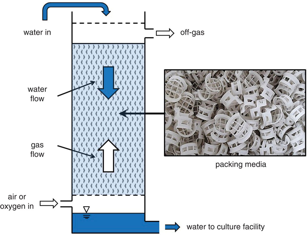
Figure 4.11 A packed‐column aerator used to aerate water and remove supersaturated gases.

Source: Reproduced with permission from Craig Tucker, 2017.

4.4.7 Clearing Pond Waters of Clay Turbidity

Muddy ponds often have low‐alkalinity, acidic water. The application of agricultural limestone and fertiliser to increase alkalinity, phytoplankton abundance and pH can cause clay particles to settle in some ponds. When liming and fertilisation are not effective, flocculating agents may be applied to precipitate suspended clay particles and clear water of turbidity. The most common agents are: organic matter, usually hay; calcium sulphate, commonly known as gypsum; and aluminium sulphate, often called alum.

The use of organic matter to treat turbidity is problematic because of the large quantities needed. The treatment rates are usually 2–3 t/ha of hay or 500–1000 kg/ha of animal manure. Such large applications of organic matter can cause depletion of DO and mortality of culture animals.

Gypsum treatment increases calcium concentration and encourages flocculation of clay particles by neutralising the negative charges on their surfaces. Gypsum must be applied at rates of 200–1000 kg/ha to achieve good turbidity removal. Depending upon the hydraulic retention time, calcium concentration will be elevated for months or even years to provide future protection against turbidity from suspended clay particles.

Alum dissolves in water to temporarily increase the concentration of aluminium ions. Aluminium ions are trivalent and more effective than divalent calcium ions in flocculating clay particles. In most water, an application of 25–30 mg/L of alum effectively removes clay turbidity. Some clays are more difficult to flocculate, so it is advisable to conduct simple tests by dosing waters with different alum concentrations to determine the effective rate.

Alum must be applied on a calm, clear day to prevent wind action or rainfall from disturbing the floc. Usually, particles of floc become obvious within 10–15 min after treatment, and the pond clears of turbidity within a few hours.

Because alum forms sulphuric acid in water, it reduces total alkalinity and lowers pH. Each milligram per liter of alum consumes about 0.5 mg/L of total alkalinity. To assure residual total alkalinity and a safe pH, alum treatment rates must not exceed the total alkalinity in concentration. For example, if the total alkalinity is 25 mg/L, the maximum, safe alum treatment is 25 mg/L.

4.4.8 Aquatic Weed and Phytoplankton Control

Plants are essential features of most pond aquaculture systems. They are the base of the food web and they function with other ecosystem components to maintain adequate water quality. For example, oxygen produced in plant photosynthesis can be a major source of DO in ponds.

Although plants are desirable in most aquaculture ponds, some species interfere with pond management, endanger the farmed animal, or impair product quality (Figure 4.12). These plants then become weeds, and aquaculturists often try to prevent them from developing or to eradicate them once established.

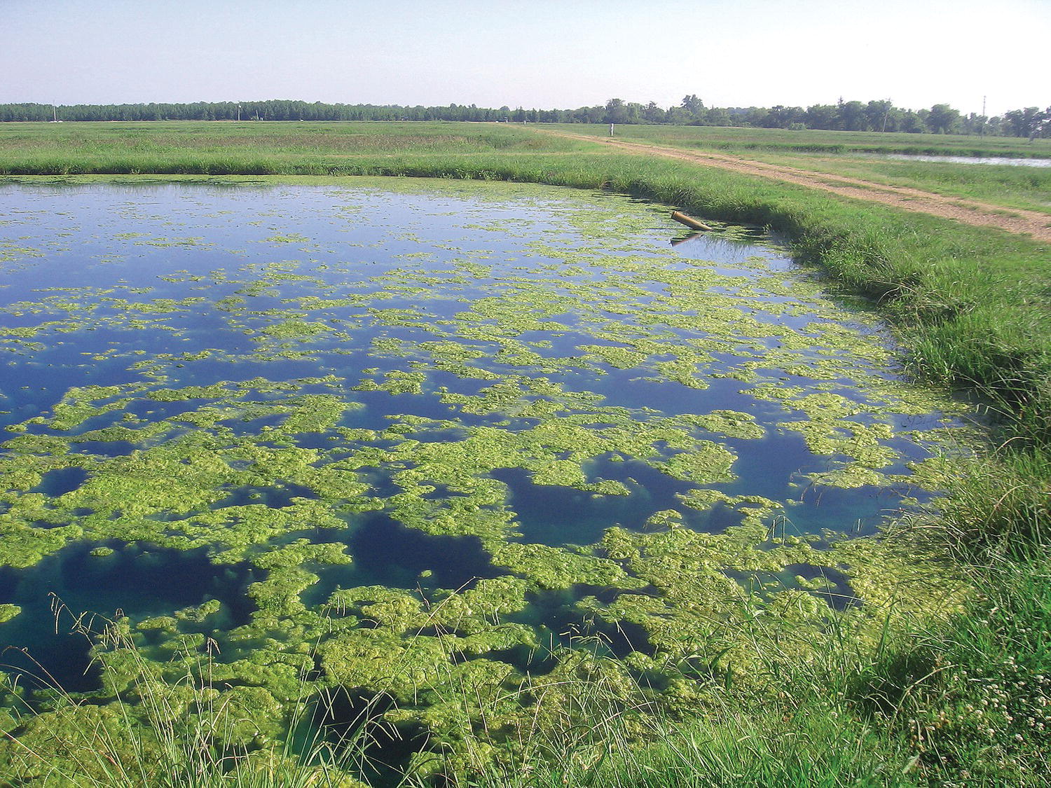
Figure 4.12 Floating mats of the filamentous macroalgae Pithophora sp. growing in a freshwater fish pond. Mats of algae and dense stands of submersed plants make it difficult to harvest or feed pond‐grown fish.

Source: Reproduced with permission from Craig Tucker, 2017.

4.4.8.1 Control of Vascular Plants and Filamentous Macroalgae

Ponds must be managed to reduce opportunities for weed growth rather than relying on herbicides to treat problems after they develop. The most common approach to weed control is fertilising ponds to encourage phytoplankton growth at the expense of other plant types. Deepening the edges of ponds also helps by discouraging the establishment of shoreline emergent or submersed weeds. Non‐toxic dyes can also be used to inhibit the growth of submersed plants by shading the water. Removing weeds mechanically or by hand may reduce the possibility of having to use other control measures but is possible only in small ponds and is seldom an option in commercial aquaculture.

Certain fish, most notably grass carp, have been used for weed control. Grass carp feed almost exclusively on larger plants and when used at low densities (25–50 fish/ha) for weed control they do not compete with other fish for feed. Grass carp are banned or tightly regulated in some countries. Several species of tilapia consume macrophytic filamentous algae and submersed plants as parts of their omnivorous diets. However, the tendency for tilapia species to overpopulate ponds is a major drawback to their use for weed control. Tilapias also do not tolerate cold water temperatures and must be restocked each year if weeds persist in temperate ponds.

Using chemical herbicides is usually the quickest way to eradicate established weed communities. Many chemicals have been used to control aquatic weeds but relatively few are legal to use in aquaculture ponds. Lists of legal herbicides differ among countries and legal status changes over time, so we will not discuss individual herbicides. Printed and online resources for aquatic plant management are abundant.

Effective herbicide use depends on correctly identifying the weed problem, selecting the most cost‐effective chemical, proper application and managing the effects of herbicide use on water quality. Correct weed identification is critical because herbicides effective on one species may be ineffective on other species. Even if the proper herbicide is selected, failure to use herbicides properly can result in poor weed control; risks to people, the aquaculture crop, or wildlife; or herbicide residue problems in the aquaculture product. The label provides information on the active ingredient, directions for correct use on target plant species, warnings and use restrictions and safety and antidote information.

With a few exceptions (copper‐based herbicides, for example), most aquatic herbicides are not very toxic to aquatic animals. However, herbicide use is dangerous because treatment of plant‐infested ponds causes dramatic deterioration of water quality. Decay of herbicide‐killed plants may cause DO depletion and increased levels of dissolved carbon dioxide and ammonia. In many instances, only a portion of the pond must be treated at one time. Supplemental aeration must always be available any time herbicides are used.

4.4.8.2 Phytoplankton Bloom Management

Ponds are usually managed to promote phytoplankton and discourage other plant growth. Phytoplankton can, however, become a weed problem when community biomass becomes excessive or when certain species produce odors or toxins. Phytoplankton overabundance in fertilised ponds indicates that too much fertiliser is being applied and the solution is to reduce fertilisation. In pond cultures with feeding, abundant phytoplankton blooms and noxious blue‐green algae are a natural consequence of large amounts of nutrients excreted into the water as metabolic waste.

Algicides are used to manage phytoplankton blooms for two distinctly different purposes. First, they are used to eliminate undesirable phytoplankton species from the community. This can be relatively successful when managing algae‐related off‐flavors, but can be dangerous when treating toxin‐producing algae. Toxins stored inside algal cells are released when cells are killed and lyse, causing a sudden, and potentially dangerous, increase in waterborne toxin concentrations. The second use of algicides is to reduce overall phytoplankton biomass. This practice seems logical because excessive phytoplankton biomass is related to poor water quality, but using algicides to kill a portion of the phytoplankton community often causes worse environmental conditions than existed before use.

Copper‐containing products are the most commonly used algicides in aquaculture. The traditional copper formulation used as an algicide is copper sulphate pentahydrate, CuSO₄ · 5H₂O, containing 26% copper. Although copper sulphate readily dissolves in water, it quickly disappears from solution through precipitation and reaction with soils.

Copper toxicity to plants and aquatic animals is strongly affected by other water‐quality variables, most notably pH, alkalinity and hardness. This makes it difficult to formulate safe, effective dosages. In most waters, those three variables are highly correlated (higher alkalinity waters have higher pH and hardness than lower alkalinity waters) and general guidelines have been developed based on total alkalinity. One such guideline is to multiply total alkalinity (expressed as CaCO₃) by 0.01 to determine the algicidal dosage for CuSO₄ · 5H₂O. For example, if the total alkalinity of 135 mg/L as CaCO₃, the treatment rate would be 1.35 mg/L CuSO₄ · 5H₂O (or 0.35 mg/L as Cu). Using copper sulphate in waters with low pH (<7.5) and low alkalinity (<50 mg/L) may be dangerous even at the rate calculated using this formula.

Copper sulphate can be applied by several methods. The most common are broadcasting crystals over pond surfaces, dissolving the chemical in water and spraying the solution over the pond, and suspending copper sulphate in porous bags where aerator currents can disperse the chemical as it dissolves. Copper sulphate can also be used to treat mat‐forming algae around pond edges. The usual method is to broadcast copper sulphate crystals over algal mats.

Copper ion can be chelated with organic compounds such as triethanolamine or ethylene diaminetetraacetic acid. Chelated copper is toxic to phytoplankton, but it is not nearly as toxic as cupric ion to aquatic animals. Thus, chelated copper products for phytoplankton control can be used in acidic, low‐alkalinity waters with less fear of harming the culture species. Moreover, in high alkalinity water of greater pH, an effective copper concentration can be achieved more easily by using chelated copper products. The main disadvantage of chelated copper compounds is their high cost, which is usually several times greater than copper sulphate per unit weight of copper.

Chelated copper algicides can be mixed with water and sprayed over pond surfaces. Also, some workers mix chelated copper algicides with water and drain the solution from a boat‐mounted tank into the turbulence caused by the propeller of an outboard motor while driving the boat over the pond surface.

Boyd and Tucker (1998, 2014) provide additional information on toxin‐producing algae, off‐flavors caused by algae and phytoplankton bloom management.

4.4.9 Mineral Amendments

Several uses of mineral amendments have already been discussed. In addition, in fish hatcheries and nursery ponds, it may be necessary to increase salinity for certain species. This can be done by applying industrial‐grade, mine‐run salt which is about 96–98% sodium chloride. In some countries, brine solution (100–250‰ salinity) from coastal seawater evaporation ponds may be applied as an alternative to salt.

Saline surface and groundwaters found in some inland regions are used to culture marine and brackishwater species. These waters often have different proportions of major ions than found in seawater. In particular, low concentrations of potassium and magnesium have been associated with poor survival and growth of some shrimp and fish species. The specific requirements of marine and brackishwater species for major ions are not known, but several studies have shown that increasing potassium concentration and sometimes magnesium concentration allowed normal growth of these species. Minerals such as fertiliser grade potassium chloride (muriate of potash), potassium magnesium sulphate (Kmag^®), and magnesium sulphate (Epsom salt) have been applied to ponds to correct ionic imbalances.

4.4.10 Bacterial and Enzyme Products

Aquaculture production is ultimately limited by the capacity of the pond microbial community to treat wastes produced during culture. To intensify aquaculture production beyond that achievable in static‐water ponds, the production system must be designed or managed to increase waste‐treatment capacity. One approach to aquaculture intensification is to export wastes produced during culture and treat them in separate units of the overall culture system (as in recirculating aquaculture systems) or by discharging wastes to public waters (as in raceways and net‐pen culture).

An alternative approach to intensifying aquaculture production is to increase the capacity of the pond’s microbial community to remove or transform metabolic wastes. This is routinely accomplished, for example, by using aeration to provide more oxygen, which stimulates microbial activity (this general approach to environmental remediation is ‘biostimulation’).

Another approach is to supplement naturally occurring microorganisms by adding microorganisms grown in mass laboratory cultures or by adding enzyme preparations derived from laboratory cultures. This general approach is called bioaugmentation.

Many microbial products are aggressively marketed for aquaculture use. Specific claims for bacterial supplements include improved water quality, reduced algal growth, enhanced sediment conditions and improved aquaculture production. Enzymes are organic catalysts that can accelerate chemical reactions but are not expended in the process. Enzyme preparations used as water‐quality enhancers are usually extracts from homogenates of yeast cells, and they function extracellularly. Proponents of these products argue that adding enzymes to ponds increases the activity of extracellular enzymes and favors greater rates of waste assimilation by microbes.

Wastes in aquaculture ponds consist of uneaten feed, faeces, and remains of plankton—ordinary organic matter that readily decomposes. Decomposer organisms respond to substrate (nutrient source) and if environmental conditions are conducive, their abundance increases rapidly until substrate is depleted. Because the abundance and variety of microorganisms respond to substrate, and microorganisms capable of assimilating aquacultural wastes are always present, it seems unlikely that lack of bacteria impairs sediment and water quality. This disappointing conclusion has been verified by numerous replicated pond studies that have failed to show significant improvements in sediment and water quality in ponds or laboratory systems treated with these products.

A few studies have shown that microbial or enzyme amendments can increase fish and shrimp survival. The mechanism by which these products enhance survival is puzzling, but it is not related to water or sediment quality improvements.

4.4.11 Water‐Quality Management in Cages, Raceways and Recirculating Systems

Pond water quality and its management are complex because all biological, chemical and physical processes are affected by external factors such as sunlight, water temperature, wind, rainfall and others. These factors vary hourly, daily and seasonally, and are difficult or impossible to control. Water‐quality management in cages, raceways and recirculating systems is much simpler, although the engineering technology used to manage the system may be sophisticated. Design and management of these systems are presented in Tidwell (2012).

Cages are enclosures used to hold and grow fish (Figures 4.13 and 3.6). They may be located along a shore or pier, or anchored and floating offshore, either in fresh or salt water. Environmental conditions inside cages (and therefore potential fish yield) depend on the quality of the surrounding water and the rate of water flow through the cage. Water flow is induced by tides, surface currents, and other natural water movements that provide a continual supply of high‐quality water and sweep away wastes produced during culture. The only control the culturist has over water quality is selecting good sites based on long‐term records of water quality, climate, current velocities and other conditions.

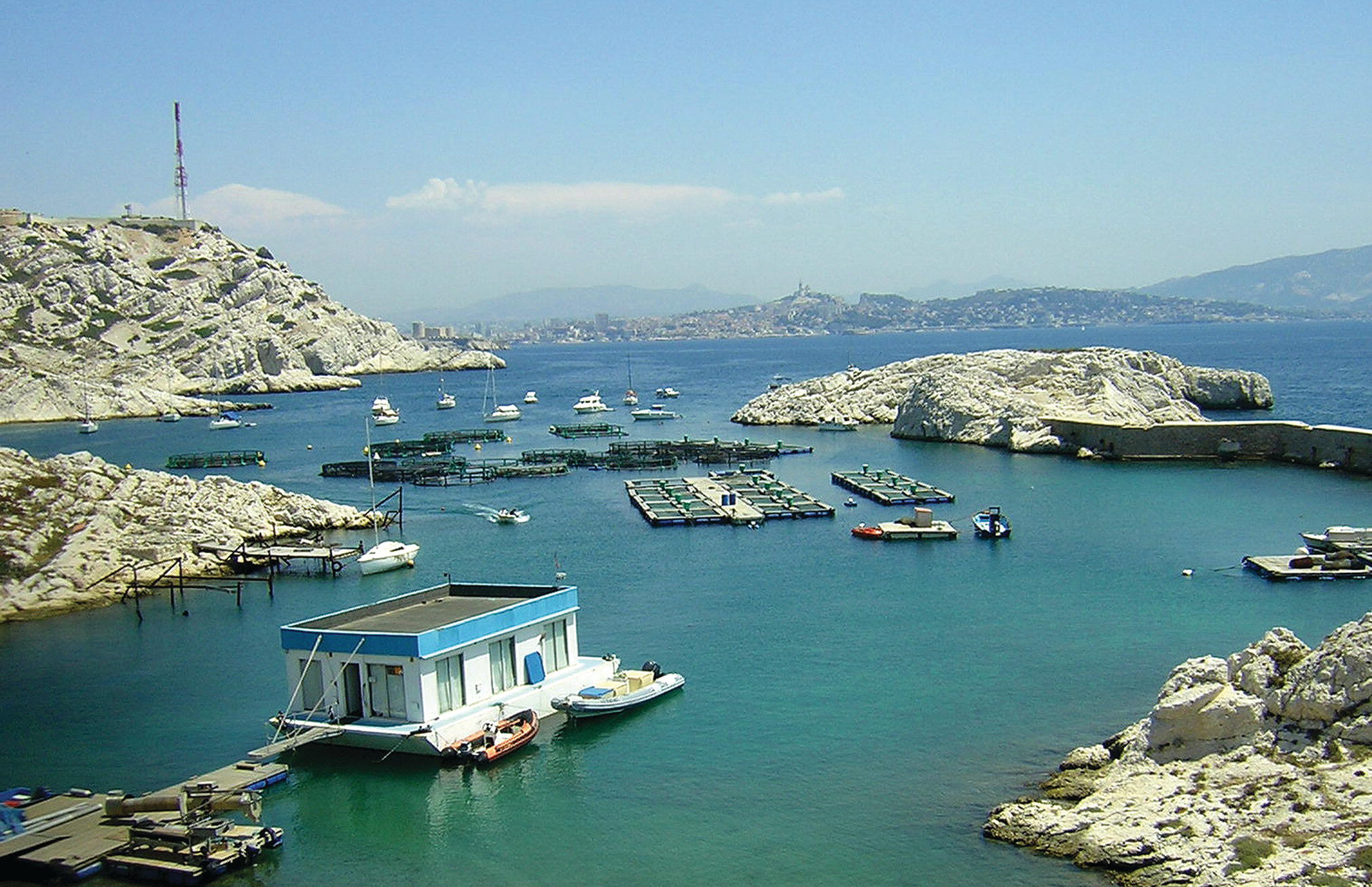
Figure 4.13 Cage culture of European seabass (Dicentrarchus labrax) and gilthead seabream (Sparus aurata) near Marseille, France.

Source: Reproduced with permission from John Hargreaves, 2017.

Flow‐through systems consist of raceways, tanks, or small ponds with water passing once through the culture unit (Figure 4.14). Water entering the culture unit provides DO, and water leaving carries away waste products. Water may be reconditioned and reused as it passes through a series of culture units, but unlike recirculating aquaculture systems, water is not reconditioned and passed through the same unit more than once. Fish production is a function of flow rate because water flow determines the amount of DO available to meet fish metabolic demands and the rate at which wastes are diluted. For trout and salmon aquaculture, which is the most common type of flow‐through aquaculture, relationships between production and water flow are refined to the point where facility design and production decisions are easily calculated.

Figure 4.14 A large flow‐through aquaculture facility used to grow rainbow trout (Oncorhynchus mykiss) in the Snake River Canyon, Idaho, USA. The facility is supplied with artesian springwater with a year‐round temperature of 15 °C flowing freely from several springs in the canyon wall. Water is diverted through the raceways and is discharged into the Snake River in the foreground.

Source: Reproduced with permission from University of Idaho Aquaculture Research Institute, 2017.

Production in flow‐through systems can be increased by providing supplemental oxygen, either by aeration (exposing water to air) or oxygenation (exposing water to pure oxygen). Oxygen can be supplied directly to the culture unit or to water flowing between culture units when units are arranged in a series. Aeration in serial raceways is usually accomplished by gravity fall over weirs between individual raceways. Production cannot be increased infinitely by providing supplemental oxygen because water‐quality variables other than DO, such as accumulation of ammonia or dissolved carbon dioxide, eventually affect fish performance.

Recirculating aquaculture systems (RAS) confine fish in tanks at very high densities. Oxygenated water flows into the tank and water containing fish wastes flows out. A large portion of the water flowing from the culture tank is recycled back to the tank after DO is added and waste products are removed.

Rapid fish growth is obtained by providing high‐quality feeds and maintaining optimum environmental conditions for growth and health. Water temperatures are controlled throughout the year (RAS are usually indoors), and rates of oxygen use and waste production can be estimated with good accuracy. These rates can be used to precisely design systems that incorporate a series of unit processes, each engineered to perform a certain task (Fig. 4.15). Particulate solids are removed by filters, toxic dissolved nitrogen compounds are removed by bacterial nitrification in biological filters, carbon dioxide is removed by gas strippers, and oxygen is added by aerators or oxygenators. Processes to control pH and alkalinity, remove nitrate and dissolved organic matter, and disinfect the water may also be required depending on production goals and the species farmed. In most facilities, monitoring and control devices oversee important processes so that environmental conditions never deviate from acceptable ranges.

Figure 4.15 Processes used to recondition water in recirculating aquaculture systems.

Reproduced with permission from Craig Tucker, 2017.

4.5 Effluents

Discharge from extensive aquaculture facilities are low in concentrations of nutrients and organic matter. Thus, they are usually not considered a significant source of pollution to receiving waters. Fertilisers and feeds are applied in semi‐intensive and intensive culture, and effluents from these systems have a greater potential for causing water pollution.

Feed is the main source of nutrients in aquaculture discharges. The fate of the nutrients and other wastes depends upon the type of culture system. In static ponds, water remains in ponds for long periods and natural processes degrade organic matter, nutrients are sequestered in sediment, ammonia diffuses into the air, denitrification returns nitrogen to the air, and suspended solids settle out. A portion of the wastes enter natural waters when overflow occurs following rainfall or when ponds are drained for harvest. Nevertheless, static ponds tend to serve as sediment traps, and a relative small percentage of the carbon, nitrogen and phosphorus applied in feed is discharged. For example, the discharge from channel catfish ponds contained about 3.1% carbon, 28.5% nitrogen and 7.0% phosphorus applied in feed (Boyd and Tucker, 1998).

In ponds with water exchange, the hydraulic retention time is less, and natural processes have less time to remove suspended solids, organic matter, and nutrients resulting from aquaculture. For example, a typical watershed pond in the southeastern United States will usually discharge two or three times its volume during the winter and early spring, and discharge little or no water during the rest of the year. Most of the feed is applied during warm months when discharge is minimal. However, in a coastal shrimp pond in Central America, water may be exchanged at a rate of 5–10% of pond volume per day flushing ponds completely within 10–20 days.

In flow‐through culture systems, culture units are flushed many times per day. In trout raceways, it is not uncommon for raceway units to be flushed three times per hour. It is possible to remove uneaten feed and faeces that settle in ‘quiescent zones’ at the ends of raceways, but suspended solids and nutrients pass through the system into natural waters.

In cage culture, all of the feed ingredients not converted to fish biomass and removed at harvest enter the water body into which cages are installed. Some of the solid waste is heavy enough to settle to the bottom beneath the cages while some of the lighter solids remain suspended in the water. Fish excrete ammonia, carbon dioxide and other wastes that enter the water as soluble nutrients.

There are two types of water re‐use systems. Outdoor systems recycle water from grow‐out units into treatment ponds and the water is eventually returned to the culture units. These systems will discharge when heavy rainfall occurs. Indoor systems rely on waste‐treatment devices such as settling basins, mechanical filters, foam fractionators, biological filters, etc. However, they will discharge to the outside when basins and filters must be cleaned and when freshwater must be added to dilute TDS (salinity) concentration that increases over time.

In recent years, there has been increasing concern about negative impacts of aquaculture effluents on natural water bodies into which they are discharged. Many governments have developed regulations to limit the volume and improve the quality of aquaculture effluents. Limits for concentrations of selected water‐quality variables and discharge volume have been established for aquaculture effluents in some nations. Producers comply with these limits in order to discharge effluents. In other nations, best management practices (BMPs) are mandated. These practices usually include methods for reducing discharge and for assuring better conversion of feed nutrients to biomass of culture species (Tucker and Hargreaves, 2008). Many aquaculture associations have developed BMPs for voluntary adoption by their members and growing numbers of consumers in developed countries are seeking aquaculture products resulting from environmentally responsible culture methods. Several organisations such as the Global Aquaculture Alliance, the Aquaculture Stewardship Council, GLOBAL G.A.P., Friends of the Sea, and some government agencies have developed eco‐label certification programs for several aquaculture species (Boyd and McNevin, 2015).

4.6 Summary

• Water quality is a critical consideration in aquaculture. Water quality in aquaculture is managed to correct problems with the facility’s water supply, to enhance the productivity of pond systems, to mitigate water‐quality deterioration resulting from the use of manufactured feeds and to improve water quality before culture water is discharged to the outside environment.
• Source water may be of impaired quality because of low pH, high turbidity or pollution. Turbidity can be controlled by eliminating its source on the watershed or by the use of a settling basin to clarify water before use. Sources of pollution usually cannot be controlled by aquaculturists, and highly polluted sites must be avoided.
• Low pH can be corrected by liming in ponds or other culture units. Fertilisers are used to increase natural productivity in pond aquaculture.
• Manufactured feeds are used to promote high production of fish and shrimp. Feeding wastes impair water quality, but mechanical aeration can be applied to increase the availability of DO and allow greater production. There is no method of reducing inputs of ammonia‐nitrogen to ponds aside from lowering fertilisation rates or stocking and feeding rates. However, the natural processes of nitrification, uptake by microorganisms and volatilisation usually prevent excessive concentrations of ammonia.
• Nitrite toxicity may be counteracted in freshwater ponds by application of chloride ion. Turbidity from suspended soil particles in culture ponds can best be removed through treatment with liming materials, calcium sulphate or aluminium sulphate.
• Aquatic plants are a critical component of pond ecosystems but some plants interfere with pond management, endanger farmed animals or impair product quality. The goal of aquatic plant management is to encourage growth of certain phytoplankton at the expense of noxious plants or harmful algal blooms.
• Water quality in cages and raceways is controlled by water flow through the system to provide oxygenated water and flush away wastes. Water quality in cages is managed primarily by selecting good sites. Production in raceways is directly related to water flow but can be increased to a point by using aeration to provide more oxygen. RAS have high production potential because water quality is maintained at optimum levels using a series of discrete engineering processes to recondition water and return it to the culture unit.
• Effluents from aquaculture facilities can cause pollution of water bodies into which they are discharged. Thus, practices must be implemented at aquaculture facilities to reduce the volume and improve the quality of effluents.

References

1. Boyd, C. E. (2015). Water Quality, an Introduction, 2^nd edition. Kluwer Academic Publishers, Boston.
2. Boyd, C. E. and McNevin, A. A. (2014). Aquaculture, Resource Use, and the Environment. Wiley Blackwell, Hoboken.
3. Boyd, C. E. and Tucker, C. S. (1998). Pond Aquaculture Water Quality Management. Kluwer Academic Publishers, Boston.
4. Boyd, C. E. and Tucker, C. S. (2014). Handbook for Aquaculture Water Quality. Craftmaster Printers, Auburn, AL.
5. Boyd, C. E., Tucker, C. S. and Somridhivej, B. (2016). Alkalinity and hardness: critical but elusive concepts in aquaculture. Journal of the World Aquaculture Association, 47, 6–40.
6. Boyd, C. E., Tucker, C. S. and Viriyatum, R. (2011). Interpretation of pH, acidity and alkalinity in aquaculture and fisheries. North American Journal of Aquaculture, 73, 403–408.
7. Colt, J. (2012). Dissolved Gas Concentration in Water. Elsevier, Amsterdam.
8. Colt, J. and Bouck, G. (1984). Design of packed columns for degassing. Aquacultural Engineering, 3, 251–273.
9. Tidwell, J. H., ed. (2012). Aquaculture Production Systems. Wiley Blackwell, Ames, IA.
10. Tomasso, J. R. (1996). Environmental requirements of aquaculture animals—a conceptual summary. World Aquaculture, 27(2), 27–31.
11. Tucker, C.S. and Hargreaves, J. A. (Eds.) (2008). Environmental Best Management Practices for Aquaculture. Blackwell, Ames, IA.

Note

1 CaCO₃ is calcitic limestone and CaCO₃·MgCO₃ is dolomitic limestone, but most limestone is not pure calcite or pure dolomite. In addition to calcium silicate, silicates of the feldspar group are sources of alkalinity.