4
The Sources of Functional Contrast
The time course of several physiologic variables can be measured and mapped with fMRI. Blood oxygen–level dependent (BOLD) contrast is a measure proportional to the amount of deoxyhemoglobin in a voxel. Activation typically increases oxygenation locally, therefore decreasing the amount of deoxyhemoglobin. MRI can also be sensitized to blood volume, blood flow and/or perfusion, and can be further sensitized to hemodynamic changes at specific vessel sizes. Quantitative measures of changes in the cerebral metabolic rate of oxygen (CMRO2) with brain activation can also be derived. New methods have also shown promise in mapping vessel radius in a voxel, mapping vascular territories, and mapping baseline blood oxygenation and metabolism. Methods that are theoretically possible yet still not convincingly demonstrated are direct mapping of neuronal current changes, mapping of neuronal cell swelling with activation using diffusion-weighted imaging, and mapping of localized temperature changes. Just recently, a method that has claimed to measure elastic changes in the brain during activation was introduced at the 2017 International Society for Magnetic Resonance in Medicine Conference. In this chapter, the focus is on the established contrast mechanisms: blood volume, blood flow, blood oxygenation, and CMRO2.
Blood Volume
In the late 1980s, the ability to obtain MR images in a fraction of a second emerged with the implementation of echo planar imaging (EPI). EPI required specialized hardware and was therefore not available on most clinical scanners. Vendors, however, were developing EPI as it held promise in the domain of cardiac imaging—allowing the creation of high temporal-resolution movies of the complete cardiac cycle. As a side benefit, the seeds for fMRI were sown as EPI would prove to lend itself well to fMRI for two reasons: its speed and its high temporal stability that allowed for the detection of small transient changes.
The ability to acquire a complete image in under 50 ms, and a complete volume in under 2 sec, allowed the tracking of MRI signal changes over time—a new dimension that, before 1990, was relatively unexplored. Rather than simply collecting one static image and comparing the image contrast over space, the rapid collection of identical images over time allowed assessment of dynamic changes in contrast.
An immediate application of this ability was the imaging of the transient effects of injected paramagnetic contrast agents. One could follow the MRI signal intensity as a bolus of a paramagnetic contrast agent such as gadolinium passed through the tissue of interest. Paramagnetic contrast agents in vessels concentrate the magnetic fields around their containing vessels, setting up microscopic field distortions, causing increased signal “dephasing” and therefore attenuating the MRI signal. As a bolus of gadolinium passes through the brain, the signal intensity is attenuated in proportion to the amount of gadolinium that is present in each voxel. Once the gadolinium washes out, the signal intensity increases to previous levels. The area under these signal attenuation curves are proportional to the relative blood volume.
In the late 1980s and early 1990s, for the first time, maps of the blood volume distribution in the brain using the gadolinium bolus injection method, with high diagnostic value, could be created.1 In 1990, Belliveau and colleagues at Massachusetts General Hospital took this ability one step further and mapped blood volume changes during brain activation.2
Blood Oxygenation
It had been known for decades prior to the discovery of BOLD contrast that hemoglobin, the molecule that is essential for enabling red blood cells to carry oxygen to tissue, had unique properties. When it is bound to oxygen, it is diamagnetic, meaning it mildly repels magnetic fields. Diamagnetism is a property shared in almost equal amounts by all biologic tissue. When it releases oxygen, the hemoglobin becomes paramagnetic—having similar properties to gadolinium—and it concentrates and distorts the magnetic fields, causing signal attenuation. In fact, as deoxygenated red blood cells become less diamagnetic than plasma, veins become less diamagnetic than surrounding tissue. This difference in susceptibility at all these scales causes magnetic field distortions that lead to spins propagating at different frequencies and therefore dephasing.
In 1982, Thulborn et al. discovered that changes in blood oxygenation changed the transverse relaxation, or T2, of blood.3 A short definition of T2 is that it is the rate at which the signal decays in the plane of detection or transverse plane after it is given energy or “excited” by an RF pulse. In tissue where the T2 is longer, the signal in a “T2-weighted” scan is brighter than in tissue where T2 is shorter. T2 is the transverse decay rate as measured using a “spin echo” pulse sequence. T2* is the transverse decay as measured using a “gradient echo” pulse sequence. T2* is almost always shorter than T2, as T2* is more sensitive to spin dephasing at all spatial scales.
A change in blood oxygen saturation therefore changes the MRI signal. Blood that is more oxygenated has longer T2 than blood that is less oxygenated. It was not until 1989 that this knowledge was used to image in vivo changes in blood oxygenation. Blood oxygen–dependent contrast, coined BOLD by Ogawa et al., emerged as a brain activation method of choice.4 The first three papers showing human brain activation using BOLD were published within two weeks of each other in 1992.5
Interestingly, Ogawa predicted its utility for functional brain imaging in his earlier papers, hypothesizing that with brain activation the signal should change. However, he predicted a decrease, hypothesizing that during an increase in metabolic activity in the brain, more oxygen would be removed from the blood, thus causing a decrease in T2 and a signal decrease.6 A few years earlier, however, a paper based on positron emission tomography (PET) suggested that an increase in brain activation is accompanied by a large increase in blood flow to the active area—overcompensating for any increase in oxidative metabolic rate. Therefore, with an increase in brain activation, the metabolic rate increases, but the large increase in oxygenated blood flow to the area causes the overall oxygenation to increase despite the increase in the oxidative metabolic rate. This increase in oxygenation causes an increase in T2 and T2* relaxation times, and thereby an increase in signal in T2- and T2*-weighted sequences. In fact, this is precisely what had been seen with fMRI—an activation-induced signal increase of about 1%–5% at 1.5T when using gradient echo imaging, suggesting such an increase in blood oxygenation.
T2 and T2* decay curves are shown in figure 8. Most BOLD contrast imaging today uses T2* contrast because it is more sensitive than T2 contrast to blood oxygenation changes by at least a factor of 2 to 4. This is mostly because T2* changes pick up susceptibility-induced inhomogeneities from small to large perturbers. Spin echo sequences are more sensitive to small perturbers on the order of scale of a red blood cell. Spin echo susceptibility contrast relies on protons diffusing through the field perturbations to have an effect on the signal. In the short time that a spin is allowed to diffuse during imaging, it will more likely diffuse through small sharp perturbations from red blood cells and capillaries. Since there is more area covered by the large perturbations (i.e., larger veins), the gradient echo signal will dephase more protons and result in a larger signal change.

Figure 8 The left panel shows T2 and T2* decay curves following an excitation pulse. T2* decay is more rapid than T2. A T2*-weighted image is formed using gradient refocusing during the T2* decay—here shown at about 3 ms. A T2-weighted image is formed using a 180-degree RF pulse to refocus the magnetization. The right panel shows the relative spin echo and gradient echo sensitivity to susceptibility compartment size.
The best echo time to use in an imaging experiment intended to optimally detect changes in T2* directly comes from the fact that the signal decay is an exponential. During rest, a single exponential with decay rate T2* describes the transverse magnetization. During activation, the T2* decreases slightly, shifting the exponential decay. If one were to compare the signal between these two exponentials, one would find that the percent change between these continues to increase with TE, but the difference between the exponentials peaks at approximately the TE equal to the resting state T2*. Signal contrast is fundamentally the signal difference and not the percent change; therefore, in all fMRI studies the TE used is approximately equal to the T2* (or T2 if spin echo acquisition is used). This depiction of the optimal TE to use is shown in figure 9.

Figure 9 The graph on the left shows the transverse signal decay as a function of TE for rest and activation, assuming a baseline T2* of 50 ms and a change in T2* of about 2 ms. As a side note R2* is simply equal to 1/T2*. If one calculates the percent signal change as a function of TE, it increases linearly, as shown in the top right graph. If one calculates the difference between the two exponential decays, it peaks at about TE = T2* = 50 ms. This is the reason why, in fMRI, the TE chosen is equal to T2*, as it optimizes the signal difference that determines the functional contrast.
Blood Perfusion
BOLD was not the only functional contrast to emerge in the early 1990s. MRI-based perfusion imaging, also known as arterial spin labeling (ASL), was more developed than discovered. It is a method that allows the creation of noninvasive, quantitative baseline perfusion maps as well as maps of activation-induced perfusion changes. In fact, Kwong et al. in their first fMRI paper published in the Proceedings of the National Academy of Sciences (PNAS) in 1992 also demonstrated that a T1- (or longitudinal relaxation–) weighted scan could detect subtle T1 changes that occur with activation-induced localized perfusion changes.
T1 is a measure of the rate in which the magnetization returns to equilibrium after it is excited by an RF pulse. It is always longer than T2, as T2 is simply a measure of how quickly the signal is dephased in the transverse plane. The net magnetization may still not be fully returned to equilibrium even though it is completely dephased. If perfusing spins from outside the imaging plane enter into the plane after excitation, they will add to the longitudinal magnetization given that they are fully at equilibrium already, thus causing the overall T1 in the plane experiencing inflowing or perfusing blood to appear more fully relaxed, with a shorter T1 (more rapid return to equilibrium). If perfusion increases, T1 shortens and the signal in a T1-weighted scan gets brighter. In this manner perfusion rates can be measured using T1-weighted scans, as was done in the Kwong paper mentioned earlier.
ASL-based perfusion mapping methods do something slightly different. They “label” the inflowing magnetization and observe the effects of that label on the imaging plane. They are similar, in principle, to tracer methods applied in other modalities such as positron emission tomography (PET) and single photon emission computed tomography (SPECT) in that they involve “tagging” or “labeling” inflowing blood, and then imaging the effects of the tagged blood as it moves into the imaging plane. Instead of tagging blood with an injected contrast agent, the “tag” is provided by a spatially selective radio frequency pulse to inflowing blood, altering its magnetization. The RF tagging pulse is usually a 180 degree pulse that “inverts” the magnetization while it is outside the imaging plane. Once the blood flows into the plane of interest, the tagged blood changes the magnetization of the tissue where it is perfusing and thus interacting with the protons in the plane of interest. Perfusion images are created by subtracting images created without the tag from images with the tag. These images highlight only the signal that changed with the tag. The signal changes in each voxel of the images are proportional to perfusion.
The advantage of perfusion imaging is that it is a direct and potentially quantitative measure of activation-induced flow changes. It also provides clinically useful baseline perfusion maps—easily differentiating gray and white matter which has a difference in perfusion of a factor of 2 to 4. The disadvantages are that it is less sensitive to BOLD contrast by a factor of 4. However, it has been put forward that it is optimal for long-duration brain activation as the time series signal does not have slow drifts in it as the BOLD signal typically has. Perfusion imaging also has intrinsically lower temporal resolution because the added necessity for the “inversion” 180 degree pulse forces the repetition time (TR) to be at least 1 sec. Lastly, brain coverage using ASL methods is limited to a single slab at a time that does not fully cover the brain, so whole-brain imaging is much more cumbersome.
Blood Volume Imaging without Contrast Agents
In the early 2000s, Hanzhang Lu developed vascular space occupancy (VASO), a method for imaging blood volume changes without the need for exogenous contrast agents. The pulse sequence made use of the understanding that blood T1 (or “longitudinal relaxation”—the amount of time it takes for the net magnetization to relax back to equilibrium—typically much larger than T2 or T2*) is different from that of brain tissue. If a 180 degree pulse (a complete inversion of inflowing spins) is applied, then, after a specific amount of time depending on the T1 of the tissue or blood, the signal will start out negative and then pass through what’s known as a “null point” where it is invisible. After passing through the null point, the signal will become positive until it is fully recovered. This null-point time is different between blood and tissue, and therefore if one waits until the blood passes through the null point, there will be a signal void (from the invisible blood) that is proportional to the amount of blood in the voxel. With brain activation, the blood volume increases, which means the relative volume of the signal void will increase, thus lowering the overall signal in that voxel. Many have shown that VASO is very selective to capillary- and small vessel-specific effects—as these show the clearest blood volume changes—and therefore is proving itself useful for extremely high-resolution fMRI where layer-or column-dependent activity is desired.
Cerebral Metabolic Rate of Oxygen (CMRO2)
In the late 1990s and early 2000s, advances were made allowing the mapping of activation-induced changes in the cerebral metabolic rate of oxygen (CMRO2). The basis for such measurement starts with the understanding that blood oxygenation is sensitive to opposing influences: flow increases (increase in flow leads to localized increases in oxygenation and therefore causes an increase in signal) and metabolic rate changes (increase in metabolic rate without a flow increase would decrease oxygenation and therefore decreases signal). With brain activation, increases in localized flow outweigh metabolic rate changes such that the overall oxygenation increases and therefore signal change is positive. Normalization using a hypercapnia has evolved into a method for directly mapping changes in CMRO2. The basic idea is that when a subject is at rest yet undergoing a hypercapnic stress (5% CO2), the cerebral flow increases without an accompanying increase in activated-induced CMRO2 changes and therefore less oxygen is extracted from the blood stream than during brain activation. The ratio of BOLD signal changes to flow changes with a hypercapnic stress would be smaller than the ratio during brain activation, because with activation the increase in CMRO2 removes some of the oxygen from the blood, thus blunting the activation-induced BOLD increase relative to hypercapnic changes. By comparing the ratio of the (simultaneously measured) perfusion and BOLD signal changes during hypercapnia and during brain activation, CMRO2 changes with brain activation can therefore be derived.
The mapping of baseline CMRO2 is more difficult as assumptions about blood volume in each voxel need to be made. So far, such techniques for mapping baseline cerebral oxidative metabolic rate have not been fully developed. Progress is being made toward this goal, however; with the advancement of better calibration techniques and fewer assumptions about how venous blood volume varies with each voxel, more precise assessments of baseline CMRO2 can be made.
Since CMRO2 mapping was developed in the late 1990s, it has not caught on as an fMRI method. While quantitative information on brain oxidative metabolism potentially could be useful, the method is cumbersome, involving CO2 breathing, division of two noisy measures, and a specialized pulse sequence.
In the first section of this chapter, we provided an overview of fMRI contrast mechanisms. Now we will delve more into the empirical characteristics of fMRI contrast: its specificity, latency, magnitude, and linearity. These characteristics define the limits and potential of fMRI—the very limits of what we can do with the signal. Understanding what influences these limits is essential to a deeper appreciation of all aspects of fMRI and for effectively designing, carrying out, processing, and interpreting fMRI experiments.
Hemodynamic Specificity
The goal in all hemodynamic measures of brain activation is enhanced sensitivity to smaller vessels, which are more proximal to regions of activation. Larger vessels are more upstream (arteries) or downstream (veins) and may lead to a spatial misrepresentation of the true area of activation. They may also lead to misinterpretation of the magnitude of the signal change for a given oxygenation change, as the magnitude of the fMRI signal change is proportional to the venous blood volume in each voxel. Figure 10 depicts graphically this concept by showing how each voxel contains within it a different proportion of arteries, arterioles, capillaries, venules, and veins, and, accordingly, a different blood volume from each vessel. This will result in a large difference of fractional signal change—up to an order of magnitude difference—for a given blood oxygenation change. This underlying variation in voxel-wise vasculature distorts the activation and causes spatially varying delays as different parts of the vasculature become oxygenated at different times as blood flows downstream.

Figure 10 Depiction of the sampling of the vasculature in an echo planar image with voxel dimensions on the order of 1–3 mm3. For a given oxygenation change, each voxel will show not only a different signal change magnitude, but likely also a different hemodynamic latency.
While the spatial certainty concern has been raised over the years, it has not been a major obstacle for the success of fMRI as, typically, blobs of activation on the order of 1 cm, obviate the need for capillary-level precision. Recently this concern has been raised as high field imaging (and the sensitivity it brings) has allowed extremely high-resolution fMRI to be carried out such that noncapillary upstream or downstream signal changes would severely skew the spatial location of activation. If one is trying to delineate activity between the surface or layer activity and the deeper, layer-dependent activity of a segment of cortex, a spatial precision on the order of <1 mm is desired, making noncapillary influences extremely problematic. In particular for layers, there is always a blood volume gradient that goes from the surface (pial vessels) to the deeper regions (more capillaries).
It is useful to give an abbreviated summary of the hemodynamic specificity of fMRI methods. With regard to choosing the right acquisition scheme or pulse sequence for optimizing sensitivity to capillary effects, there are other factors in play that require some thought regarding trade-offs. These include the general principle that the more sensitive the sequence is to capillaries the lower sensitivity it will have overall since capillaries fill at most about 2%–4% of a voxel while larger vessels may fill a voxel 100%. Also, several capillary-sensitive techniques such as VASO and ASL are limited in spatial coverage (they can only cover a few slices per acquisition) and time (the added “inversion” pulse adds to the overall time per image, thus lengthening the TR or time between each image acquisition).
Regarding BOLD contrast-dependent functional imaging, spin echo sequences are more sensitive to small susceptibility compartments (capillaries and red blood cells) and gradient echo sequences are sensitive to susceptibility compartments of all sizes. A small amount of diffusion weighting, or “velocity nulling,” reduces the intravascular signal therefore reducing, but not eliminating, large vessel effects in gradient echo fMRI, but eliminating all large vessel effects in spin echo fMRI. At very high magnetic fields such as at 7 Tesla, blood T2* is very short—much shorter than the T2* of tissue. Therefore, even without diffusion weighting, intravascular signal is extremely small, so that spin echo sequences at high field are sensitive to capillaries without the need for additional measures to minimize intravascular signal. In general, with an increase in field strength, BOLD contrast increases linearly to slightly super-linearly and overall image signal to noise ratio increases linearly; therefore, higher field is desired for fMRI based on BOLD contrast—especially at high resolution.
Perfusion imaging is generally accepted to be more specific to brain activation-induced hemodynamic changes in capillaries, but perfusion methods also can suffer from intravascular signal contamination from larger inflowing arteries and arterioles. As mentioned, it has also been shown that VASO methods are highly selective to capillary effects—allowing precise localization to small regions of brain activation, demonstrating layer-dependent activity with sensory-motor tasks.
In almost all fMRI studies that have been performed, the need for sensitivity has consistently outweighed the need for specificity greater than 1 cm. With studies performed at high field and high-resolution fMRI, specificity carries more importance, and therefore there has been a renewed interest in further developing sequences that are more specific to capillary effects that are most proximal to true neuronal activation, even if sensitivity is sacrificed somewhat.
The Hemodynamic Transfer Function
The hemodynamic transfer function is referred to here as the combined effect on the fMRI signal change shape, latency, and magnitude by the neuronal-vascular coupling, blood volume, blood flow, blood oxygenation, hematocrit, and vascular geometry, among other variables. A goal of fMRI method development is to completely characterize this transfer function as it varies across subject populations, individual subjects, regions in the brain, and even voxels. A more ambitious goal is to not only characterize this variability, but to also develop robust calibration methods such that studies may “look through” this variability to derive more specific information from BOLD contrast.
Characterizing the transfer function is challenging because the variables previously listed all can contribute and vary among subject, brain region, and voxel. The very idea of a transfer function also assumes a linear system, which to a first approximation characterizes the hemodynamic response. However, it tends to behave nonlinearly, providing more contrast than expected with very brief (<3 sec) or very weak neuronal activation.
The goal is to allow fMRI to make more precise inferences about underlying neuronal activation location, magnitude, and timing. The ultimate limits of fMRI depend on being able to make maps of these variables—allowing spatial normalization and more precise inferences about neuronal activity. This is particularly relevant when attempting to compare subject populations or individuals where these hemodynamic effects might vary. For instance, a medication may vary fundamental mechanisms of neurovascular coupling in a patient, thus rendering any interpretation of differences in BOLD contrast between the patient and a nonmedicated normal volunteer problematic. The issue of characterizing the hemodynamic transfer function is also relevant when attempting to infer such things as precise timing or causality between regions (i.e., how one region acts on or is acted on by another) where the hemodynamics may vary from voxel to voxel.
After the onset of activation, or rather, after the neuronal firing rate has passed an integrated temporal-spatial threshold, either direct neuronal, metabolic, or neurotransmitter-mediated signals reach arteriole sphincters, causing dilatation. The time for this initial process to occur is likely to be less than 100 ms. After vessel dilatation, the blood flow increases by 10%–200%. The time for blood to travel from arterial sphincters through the capillary bed to pial veins can be up to about 2 to 3 sec. This transit time determines how rapidly the blood oxygenation saturation increases in each part of the vascular tree. Depending on which part of the vascular tree is predominantly captured by each voxel, the latency, shape, and magnitude of the hemodynamic response might vary significantly. A typical hemodynamic response function is shown in figure 11. This function is typically modeled as a Gamma Variate function. This transfer function, in humans, is noted for a peak occurring about 5 sec after the onset of stimulation, and a post undershoot that follows activation.
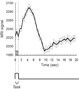
Figure 11 This is a depiction of a hemodynamic transfer function, otherwise known as the impulse response function. For most task durations >3 sec, the hemodynamic response behaves in a linear manner and therefore can be described fully by this function. To predict fMRI time series, this function is convolved with the neuronal input function.
Location Specificity
In resting state, hemoglobin oxygen saturation is about 95% in arteries and 60% in veins. The increase in hemoglobin saturation with activation is largest in veins, changing from about 60% to 90%. Capillary blood oxygenation changes from about 80% to 90% saturation. Arterial blood, already saturated, shows virtually no oxygenation change. This large change in saturation in veins is one reason why the strongest BOLD effect is usually seen in draining veins.
The second reason why the strongest BOLD effect is seen in draining veins is that, as mentioned, activation-induced BOLD contrast is highly weighted by blood volume in each voxel. Since capillaries are much smaller than a typical imaging voxel, most voxels, regardless of size, will likely contain about 2%–4% capillary blood volume. In contrast, since the size and spacing of draining veins is on the same scale as most imaging voxels, it is likely that veins dominate the relative blood volume in any voxel that they pass through. Voxels containing pial veins can have 100% blood volume while voxels that contain no pial veins may have only 2% blood volume. This stratification in blood volume distribution, illustrated in figure 10, strongly determines the magnitude of the BOLD signal.
Different fMRI pulse sequences can give different locations of activation due their different sensitivities to specific vasculature. The ASL-based perfusion change map is sensitive primarily to capillary perfusion changes, while the BOLD contrast activation map is weighted mostly by veins near the activated region. For high-resolution studies, pulse sequences such as VASO (sensitive to blood volume changes predominantly in capillaries) and spin echo sequences (sensitive to small compartments including capillaries) at high field increasingly are being used to detect very small regions of activation.
In spite of the hemodynamic limitations of these methods, detailed activation at the cortical column level7 and the laminar level8 have been reported using BOLD contrast.
Latency
One of the first observations made regarding fMRI signal changes is that the BOLD signal takes about 2 to 3 sec to begin to deviate from baseline following the onset of activation. Since the BOLD signal is highly weighted toward venous oxygenation changes, with a flow increase, the time for venous oxygenation to begin to increase will be about the time that it takes blood to travel from arteries to capillaries and draining veins—about 2 to 3 sec. The hemodynamic “impulse response” function, as described, has been effectively used to characterize much of the BOLD signal change dynamics. The use of this function to predict the hemodynamic effect from all stimuli timings assumes the system is linear, which holds for most time scales but appears to deviate with stimuli durations shorter than about 3 sec. Regardless of this nonlinearity, observed hemodynamic response to any neuronal activation can be predicted with a reasonable degree of accuracy by convolving the expected neuronal activity time course with the BOLD “impulse response” function.
Early on, it was observed that BOLD latencies varied up to 4 sec in the brain. The variation was not as much between regions but more distributed across voxels. These latencies were also shown to correlate with the underlying vascular structure. The earliest onset of the signal change appeared to be in large-vein-free gray matter and the latest onset appeared to occur in the largest draining veins. Similar latency dispersions in the motor cortex and other areas have been observed.
As a side note, the overall latency distribution of resting state fluctuations has been shown to vary between gray and white matter and with vasculature. In fact, this method of observing latency with resting state has been implemented clinically to assess regions of stroke or compromised vasculature. Areas that are compromised have more delayed effects and therefore longer latencies in their baseline fluctuations.
Methods for working around these spreads of latencies in the context of fMRI to delineate cascaded brain activity with cognitive tasks have included forcing specific cognitive components of tasks to be long (on the order of several seconds) so that they may be differentiated, or by simply looking at the change in the latency with specific and task timing changes. In the latter studies, the absolute latencies are not mapped but, rather, the spatially specific changes in latencies are determined as they correlate with the task timing modulation. Using the latter approach of looking at changes, either in latency or width, task timing modulations of as low as 50 ms have been discerned.9
Regarding the hemodynamic response itself, it seems to be quite sensitive to transient neuronal activity. Stimulus durations as low as 16 ms (limit of the refresh rate of the stimulus apparatus) have been shown to elicit a response.
Magnitude
The magnitude of the fMRI signal change is influenced by several non-neuronal variables that may vary across subjects as well as across voxels in each subject’s brain. Within subjects, it varies from voxel to voxel, thus influencing the voxel-averaged magnitude across activated regions as well as the activation pattern within activated regions. A complete and direct correlation between neuronal activity and fMRI signal change magnitude, in a single experiment, will remain nearly impossible until all the variables can be characterized and/or calibrated on a voxel-wise basis. Because of these physiologic variables, brain activation maps will typically show a range of BOLD signal change magnitude from 1%–10% for any given stimulus. Typically, large vessel effects show much higher fractional signal changes, so a crude method to remove large vessel effects is to simply establish the threshold based on an upper bound of percent change. Regarding the interpretation of the magnitude of the fMRI signal change, the picture is not that bleak. Progress has been made in successfully characterizing the magnitude of the fMRI signal change as it varies with the degree of neuronal activity variations. Like modulating timing to see differences in latency with a timing variation, the signal change magnitude is commonly modulated in a systematic manner so that the influence of intrinsic hemodynamic weighting is minimized. Such experiments are commonly referred to as parametric designs and are quite powerful as any non-neuronal influences, including vascular structure as mentioned, do not change with neuronal activation and therefore can be subtracted.
Many studies have been published that have increased our confidence that BOLD magnitude is indeed able to be altered by a systematic modulation in the amount of neuronal activity. Inferred brain activation modulations—visual cortex modulation by altering the flicker rate or contrast of the display; motor activation modulation by altering finger tapping rate; and auditory cortex modulation by altering syllable rate—have resulted in clear monotonic BOLD signal change correlations. Parametric experimental designs represented a significant advance in the way fMRI experiments were performed, enabling more precise inferences about the BOLD signal change with task modulation.
The magnitude of the fMRI signal change is influenced by several non-neuronal variables that may vary across subjects as well as across voxels in each subject’s brain.
In the early 2000s a seminal paper by Logothetis et al.10 demonstrated a clear relationship between electrophysiological measures and BOLD contrast. Simultaneous collection of multi-unit-recording array data and BOLD-based fMRI data was carried out in primate-visual-cortex visual stimulation with a flashing checkerboard of varying contrast. The study demonstrated an approximately linear relationship between local field potential power and BOLD contrast—within a range of stimulus contrasts. However, the relationship became highly nonlinear at low levels of stimulation, where the BOLD signal overestimated the amount of neuronal activation. The linearity of BOLD responses can be considered in different ways, described in the next section.
Linearity
Here we delve a bit more into the BOLD signal as it behaves as a function of task timing and intensity. As mentioned earlier, it has been found that with very brief stimulus durations, the BOLD response shows a larger signal change magnitude than expected from a linear system. This greater than expected BOLD signal change is specific to stimuli durations below 3 to 4 sec. Figure 12 shows this greater than linear response behavior. Reasons for nonlinearities in the event-related response may be neuronal, hemodynamic, and/or metabolic in nature. For instance, it has been shown in electrophysiological measures that the neuronal response shows a large transient at the onset of activation. Nonlinearities in the response can also arise from mismatches in the timings of flow, volume, or metabolism changes. It has also been found that BOLD contrast is still detectable with an on/off oscillation of up to 0.75 Hz—also well above the threshold detectable frequency from a linear model of the hemodynamic response.11

Figure 12 The hemodynamic response is greater than a linear system at durations below about 3 sec. Here is a depiction of actual data (solid line) and simulated data (dashed line) of the response to increasing stimulus durations (depicted by boxcars at the bottom).
BOLD contrast is highly sensitive to the interplay of blood flow, blood volume, and oxidative metabolic rate. If any of these variables has a rate of change that is different than the others, nonlinearities in the relationship between neuronal activity and BOLD may be manifest.