5
Hardware and Acquisition
An extensive review of the physics and engineering underlying the acquisition of the rawest signal coming off the scanner and the creation of MR images is beyond the scope of this book. This chapter offers instead a basic, practical understanding of MRI hardware and acquisition suitable for anyone working with or interested in fMRI. So much of the signal as well as the artifact is tightly tied to the details and subtleties of how the scanner itself works and how the data were acquired. This chapter provides information and guidance to encourage readers to better design and carry out experiments and to have more useful conversations with individuals engaged in the fMRI acquisition process.
First, it’s important to put almost all of fMRI technology in perspective. MRI technology has almost completely been driven by the powerful, clinic-based MRI market—and the same is true of fMRI, which uses clinical MRI systems with clinically-focused pulse sequences. However, MRI systems were not designed with fMRI in mind, which means that while the field of fMRI has benefited from this relationship, in many ways it is also limited by it.
MRI technology has been developed by academic centers in close contact with the industry leaders in MRI (principally Siemens, GE, Philips), then incorporated into the clinical scanners and distributed for clinical use. However, innovation for most fMRI technology has taken a slightly different route. Typically, fMRI R&D has been carried out by academic labs with engineers or physicists who have the skills and interest to modify MRI clinical pulse sequences, image reconstruction methods, and hardware such as RF coils and gradient coils. Since the current market for fMRI is only a fraction of the entire MRI market, research-directed innovations that do not spill off from clinical market-focused innovation tend to come from academia. These academic-driven innovations typically translate into a widely distributed product only if they are seen to benefit a more clinically relevant application. However, many if not most fMRI innovations in acquisition are the by-product of collaborating researchers, waiting to be converted into something that a wider range of people can use. Functional MRI as a field will advance significantly if vendors invest more time and money in developing better systems optimized specifically for fMRI.
Functional MRI as a field will advance significantly if vendors invest more time and money in developing better systems optimized specifically for fMRI.
In the sections that follow, this chapter describes the practical nuts and bolts of MRI technology: The primary magnetic field (B0), Radiofrequency (RF) coils, shim coils, gradient coils, and pulse sequences. An outstanding primer on all these variables also can be found in the self-published book All You Really Need to Know about MRI Physics.1
The Primary Magnetic Field: B0
MRI is based on the fact that specific elements (hydrogen, deuterium, lithium, carbon, nitrogen, fluorine, sodium, phosphorus, and potassium) have a magnetic moment, meaning that when these elements are placed in a magnetic field (B0), they have a distribution of energy states that can be modulated by an oscillating magnetic field (B1), produced by an RF coil. Then, while in their “excited” state, these elements are measured with typically the same RF coil, now acting as an antenna. Hydrogen in water not only makes up a large fraction of the body mass but also has an extremely large magnetic moment. Therefore, almost every MRI produced is of water.
Each of these unique elements also have what is known as a gyromagnetic ratio, which determines the rate at which each element precesses or oscillates when experiencing the primary magnetic field, B0. Their precession frequency is equal to the gyromagnetic ratio × B0, known as the Larmor frequency. To give a point of reference, hydrogen precesses at about 42 MHz in a 1 Tesla field. The B1 field pulse frequency pulse has to be in “resonance” or oscillating at the same frequency that provides energy at the “resonance” frequency of the element. This frequency is serendipitously within the completely-safe radio-frequency range, hence the reason for the term for the coil that generates the oscillating field.
The amount of signal we can detect is directly proportional to the magnetic moment. It is therefore a fundamental principle in MRI that sensitivity increases with field strength, or B0, which increases the magnetic moment as it increases. Because sensitivity is a highly desired commodity in all MRI applications, and because high field strength is achievable by relatively straightforward technological advancements (i.e., more wire windings), field strength for human scanners has steadily increased since the beginning of human MRI. It should be noted that increasing field is not really that straightforward: superconducting wire technology is pushed to its very limits in the context of MRI scanner manufacturing. The wires need to be as small as possible yet able to carry the massive currents required for MRI scanners. Coolant technology needs to be robust and compact. All these factors drive up the price of high field scanners. While the current cost of high field scanners scales linearly with field strength—at approximately $1 million cost per Tesla, and a bit higher at the extreme high end and a bit lower at 1T and below—the ability to extract novel contrast more efficiently and accurately and at higher resolution increases perhaps superlinearly with sensitivity, thus maintaining the drive to high fields.
Functional contrast to noise using BOLD also scales at least linearly with field strength. The type of anatomic MRI contrast possible also becomes qualitatively different at high field. For example, phase contrast at 7T is profoundly more sensitive to susceptibility contrast. With the advantages of high field, the researcher can also trade resolution or speed, or both, with the new abundance of sensitivity. Signal to noise scales linearly with voxel volume, so the practical lower voxel-volume limit should become smaller in proportion to field strength. At 3T, about 2 mm3 voxel volumes are practically possible for fMRI; however, at 7T, 1.5 mm3 is practically possible with fMRI.
The highest field strength for human MRI had been 11.7T at the National Institutes of Health. However, that scanner “quenched.” When a magnet quenches, the supercooled superconducting wire starts to heat, thus increasing its resistance. With increased resistance, more heat is generated, thus an irreversible cascading increase in temperature commences, and an explosive “boiling off” of the liquid cryogens takes place. This process can damage the primary magnet and of course results in the loss of all of the extremely expensive liquid helium (a coolant), becoming quite costly. The 11.7T scanner was, in fact, damaged, and is now being repaired, so the highest field for now is 10.5T. The most common high field strength human scanner is 7T, with about sixty such scanners being used worldwide.
The achievement of extremely high resolution functional MRI at 7T has required innovation in several areas, given that four major challenges are manifest with higher field strength. First and foremost, transverse relaxation (T2* and T2) become shorter with high field, allowing less time for data acquisition after the excitation RF pulse before the signal decays into the noise. Second, magnetic field inhomogeneities, manifesting as signal dropout regions, are much more significant and are hard to remove. Third, RF excitation uniformity throughout the brain becomes worse. Without correction, RF flip angles vary from region to region—adding uncertainty to the structural and even functional contrast. Fourth—less of a problem for fMRI as it is for more RF intensive sequences—RF power deposition increases with increases in B1. As mentioned, at higher fields, higher RF frequencies are needed to “excite” the protons—a first step in creating MR images. With higher frequency, increased RF power is necessary, resulting in potential tissue heating for high RF duty-cycle sequences, thus limiting the RF duty cycle in certain sequences for high-resolution anatomic imaging. Commercial scanners have an upper limit of RF power allowed, keeping the “specific absorption rate” (SAR) well below the level that would lead to tissue heating.
Many solutions or at least partial solutions to these challenges have been implemented. More rapid acquisition methods have helped to compensate for the fact that the signal dies away more rapidly at high field (short T2* and T2). To compensate for signal dropout, shimming hardware and techniques have generally improved and smaller voxels generally reduce any signal dropout. RF uniformity issues have been addressed by calibration scans in addition to new technology that allows adjustment of RF power from each coil “element” enabling “smoothing out” of the power distribution in the brain—also known as “RF shimming.”
The achievement of extremely high-resolution fMRI at high fields has also introduced new challenges regarding how to average and compare fMRI data. Typical practice in the past has involved spatial smoothing, spatial normalization, and averaging of functional activation maps of multiple subjects. Performing spatial smoothing on high resolution removes the benefits of collecting at high resolution in the first place. Also, spatial variability of fine structures increases with increased resolution. It’s much easier to spatially average large swaths of brain across subjects than to average, for instance, cortical columns. Large swaths of brain activation are similarly distributed across subjects, but finer details of activation have much more variability, defying spatial averaging. Rather than collapsing and comparing data spatially, it is likely possible to collapse and compare in other data dimensions or perhaps locally along columns or layers, thus keeping the detailed high-spatial-resolution information. Such innovations have yet to be fully realized. High resolution also represents a paradigm shift in that the research focus is on individual results with high resolution rather than spatially averaged group results coming from low-resolution scans.
Radiofrequency Coils
Radiofrequency (RF) coils provide the oscillating field that “excites” the protons that are imaged and also receive the signal from the protons as the energy is released, providing the signal from which the image is created. The larger the RF coil, the less sensitive it is to the signal. However, generally speaking, the larger the RF coil the more uniform the excitation field. Innovations in RF coil engineering have mainly entailed decreasing the size of the coils and adding more coils around the head or body. If multiple receiver coils are added, typically a separate single RF coil is used for excitation. Recently, multiple coils have been used for excitation as well. Adding more coils has several advantages. First, sensitivity is increased since there are many sensitive small coils rather than one less sensitive large coil. Second, certain pulse sequences actually use the coil position to help create the image itself—allowing the data to be collected more rapidly. This improvement results in either higher resolution, more signal (as a shorter echo time or “TE” can be used when a shorter readout window is possible), or more rapid collection of whole-volume data sets.
By the early 2000s, eight channels—or separate coils—were added and then, by about 2006, sixteen and thirty-two channels were added. Currently, up to 128 RF coils have been used. In fact, a novel acquisition scheme known as “inverse imaging” (INI) has been used to virtually eliminate the need for spatial encoding gradients, thus substantially increasing the temporal resolution as well as decreasing the acoustic noise associated with acquisition, since gradient switching—essential for standard imaging formation—is what contributes to the high level of acoustic noise associated with MRI.
A second innovation in RF coils is on the excitation side. Technology for multichannel excitation has been in existence for over twenty years, yet only recently has it been used in conjunction with RF shimming methods that allow a uniform RF excitation profile to be obtained by adjusting each individual coil’s power. This area is still in its infancy, since with multiple RF coils there is a danger of establishing RF “hot spots” in the brain where coil excitation fields overlap. Mitigation of this danger requires modeling of the head structure and accounting for any possible variation in head structure across individuals. This problem has not yet been fully resolved.
Gradient Coils
To review, the primary magnetic field B0 causes the protons to precess at a specific frequency and is necessary for the creation of a “magnetic moment” that is the source of the signal. The oscillating RF field, B1, is resonant with the precession frequency (in the RF range) and “excites” the protons. After a short time following the pulse of RF power, the protons start to “relax” and give off signal that is detected by the receiver coils in the transverse plane. At this moment, the signal needs additional “encoding” to be turned into an image. The basic principle at work is that the precession of the signal is directly proportional to the magnetic field that it is experiencing. In order to differentiate the signal in space, spatial gradients in the magnetic field have to be created rapidly, using a gradient coil. If a coil creates a gradient in space, we now have the protons precessing at a frequency and phase that is specific to their location in space. Once the signal is finally collected during spatial encoding, an algorithm known as the Fourier transform is applied to the data to create the image.
For high-speed imaging, the gradients need to perform this spatial encoding, line by line, in about 30 ms, implying that to create a 64 × 64 or 128 × 128 matrix they have to switch at a rate above 2 kHz or 2000 times per second. The technique that involves this rapid switching of the gradients is called echo planar imaging (EPI) and is the primary sequence used in all of fMRI. With each RF excitation and subsequent “echo,” an entire plane or slice of data is created. The switching of the gradient induces large torque as it opposes the primary magnetic field, causing subtle yet loud mechanical vibrations. This is the source of the loud noise in MRI and fMRI. Typical clinical sequences collect data line by line using multiple RF pulses per plane, however EPI collects all the lines in one plane at once. When having EPI performed, the subject hears a “beep” sound for each image. These beeps are about 2 kHz.
In the very early days of fMRI, EPI could only be carried out at a resolution of about 3 mm3 in two ways: The first was with the use of a “resonant” gradient amplifier system (i.e., ANMR) that was retrofitted onto an otherwise standard scanner. The second was with the use of low inductance, home-built head-only gradient coils. The home-built gradient coils helped deliver extremely high gradient switching rates (up to 200 mT/m/s) as well as very high gradients that are useful for high diffusion weighting. Once the major vendors implemented more powerful gradient amplifiers and other engineering improvements, local gradient coils were no longer necessary for performing EPI.
In recent years, head-specific gradient coils once again have started to make a small comeback as improved technology (hollow current-carrying wires for more efficient circulation of cooling fluid), increased need (even more gradient strength for faster imaging and higher resolution), and niche markets (head only) have entered the scene. While local gradient coils have disadvantages that include a level of added confinement, awkwardness for patients/subjects, and a more nonlinear gradient profile, they do have several advantages. Their lower inductance allows faster switching and higher gradients for a given current. Also, as the gradient falls off rapidly outside the coil, the change in magnetic field per unit time (dB/dt)—which increases with the distance of the gradient from the pivot axis isocenter—is not as high as with a whole-body gradient coil that creates gradients much further away from the pivot axis and does not cover such critical regions as the heart. It is understood that the biologic limits of dB/dt (or the rate at which the magnetic field changes in a specific location) are well below the physical limits imposed by the gradient coil. In other words, the coils are physically capable of switching much faster, but are limited by the fact that if they switch at a higher rate muscle twitching will be induced. However, if we limit the size of the gradient coil, it is possible to have a higher dB/dt at the point where imaging is taking place without being limited by the higher dB/dt further away from the pivot axis. In spite of this, it seems that in a clinical market, local coils will not be widely used—unless the research market changes such that high speed is clinically called for.
Pulse Sequences
A pulse sequence is the list of commands that are given to an MRI scanner to create an image. The details of pulse sequences and image formation are beyond the scope of this book; however, it’s useful to have a general understanding and appreciation of what pulse sequences do because a fundamental aspect of fMRI method development is the advancement of pulse sequences for hemodynamic specificity, spatial or temporal resolution, sensitivity, or better brain coverage.
A pulse sequence generally involves a sequence of commands to the scanner to provide an RF pulse (to excite the protons so that there is signal to create an image), to create transient magnetic field gradients (to spatially encode the image), and to acquire the signal during these gradients. Specific pulse-sequence timings (adjusting when the RF pulses, gradients, and image acquisition take place) have a profound effect on the type of image contrast that is created. Depending on the pulse sequence that is played out, an MR image can highlight white matter, gray matter, CSF, water diffusion direction, and many more tissue properties. The pulse sequence also determines the image resolution and acquisition speed. It is fundamentally important to understand that the aspect of resolution and speed—as with EPI—is relatively independent to the part of the pulse sequence that influences the functional contrast.
It’s also important to discuss the EPI pulse sequence just a bit more. Because EPI collects an entire plane of data in less than 50 ms, all physiologic noise that can vary over time is “frozen” in time. Methods that take longer have an additional instability as the raw data for each image is collected across different times in cardiac and respiratory cycles, leading to “ghosting” artifacts that vary over time. EPI also has “ghosts”, but they are stable over time as each echo planar image is collected in a short enough time to “freeze” any cardiac or respiratory changes during image collection. Because of this advantage, the temporal stability improvement is substantial as well as critical to fMRI for detecting very subtle 1%–5% signal deviations associated with blood oxygenation changes.
Almost every fMRI pulse sequence uses EPI for acquisition. However, the EPI gradient readout is only part of the pulse sequence. The sequence timing and RF pulses can be adjusted to create different contrast sensitivities. In the context of fMRI, pulse sequences can be crafted to create functional contrast weightings that can highlight large vessel flow, capillary perfusion, blood oxygenation, and blood volume. These contrast sensitivities were described in chapter 4.
In the early 2000s the inception of methods for using multiple independent receiver coils to improve spatial encoding efficiency made an impact in fMRI. As described earlier, imaging encoding, typically performed by gradients, can also be carried out by using multiple independent receiver RF coil sensitivity profiles—known as SENSitivity Encoding (SENSE). These have allowed either higher resolution imaging at a given readout window length or higher speed (i.e., shorter readout window length) imaging at a given resolution. In the context of fMRI and diffusion imaging, images of at least twice the resolution typically obtained have been collected using a single-shot approach. Since single-shot imaging is essential for the high stability needed in fMRI and diffusion tensor imaging (DTI), a method for performing higher resolution in a single shot was embraced. Now a large fraction of high-resolution fMRI studies is performed using single-shot SENSE acquisition methods.
A remaining problem when collecting high-resolution images is that with such thin slices, more slices and therefore more time are required to cover the entire brain per repetition time (TR). Assuming that about 15 images can be collected in a second, if 100 very thin slices are required to cover the entire brain, then the minimum repetition time (the time between each volume) or TR required to achieve whole brain coverage would be just under 7 sec. A TR of this length would typically make high-resolution whole-brain imaging prohibitively long because a minimum number of time points typically need to be collected—especially with less SNR at high resolution—to achieve statistical significance in brain activation images.
The answer to this problem arose independently from the Massachusetts General Hospital group2 and the University of Minnesota group in collaboration with Berkeley.3 The general concept is to use simultaneous multiplexed excitation of several imaging planes, allowing slice collection speedup by a factor of up to 8. This technique generally is known as simultaneous multi-slice (SMS) imaging. Instead of 15 slices per second, it is now possible to collect up to 120 slices per second using this approach!
The highest single-shot EPI functional resolutions (<1mm3 voxel sizes) obtained have been in cortical layers and columns. Ocular dominance and orientation column activity have been mapped in humans.4 Layer-specific mapping has also been accomplished. The ability to resolve layer-specific activity is of high potential significance as it is generally known that specific layers provide an “output signal” to other parts of the brain and other layers provide an “input signal.” Teasing out this output/input directionality is a new frontier in fMRI that may shed light on what is understood about the functional circuitry of the healthy human brain.
In the direction of speed at perhaps the expense of resolution, a method involving using the RF coils almost exclusively for spatial localization, known as INI, has been developed.5 Several groups have introduced echo volume imaging (EVI) as well.6 This method allows collection of an entire volume of data in a single echo—as the name suggests. The major advantage is that motion correction works much better when the entire volume is a rigid body collected at one moment. In most cases with multi-slice imaging, through-plane motion is represented by a difficult-to-correct shearing across the volume as each slice is collected at a different time during the motion.
Pulse sequences can be designed and used to minimize time series noise. A recent example of this facet of innovation concerns multi-echo gradient echo EPI acquisition for fMRI time series. BOLD signal changes are fundamentally manifest as changes in T2* while most artifactual signal changes do not involve changes in T2*. Change in T2* cannot be differentiated from non-T2* changes using a single echo for acquisition—as most fMRI time series obtain. Multi-echo acquisition, involving at least two readout windows per excitation along the T2* relaxation curve, allows baseline and activation-induced changes in T2* to be characterized and separated from artifact. Kundu et al. have developed an approach in which three-echo EPI time series are collected. 7 From this time series, independent component analysis (ICA) is applied. Each component can be analyzed across each TE to determine how well it fits into the T2* change curve. If the signal is BOLD based, the percent signal change will increase linearly with TE. If it is not BOLD, then the percent signal change will show no clear relationship to TE. The quality of fit for each ICA component is then calculated and ranked. From this ranking, a clear delineation of BOLD ICA components versus non-BOLD ICA components can be made.
A final pulse sequence innovation described here involves minimizing scanner acoustic noise. A major challenge in fMRI has been that the scanner is extremely loud, interfering not only with the presentation of acoustic stimuli but also with the interpretation of the acoustic-related brain activation. One answer to this problem was a development known as clustered volume acquisition. Rather than collecting an entire volume with each slice evenly spaced in time to continuously fill the acquisition time between volumes, the slices instead were “clustered” in time. For instance, if a TR were 4 sec, each volume would not take 4 sec to collect but rather, the entire volume would be collected in 1 sec, followed by 3 sec of silence. The TR itself was not altered, but now there was a period of silence that would allow subtle auditory stimulation.
Another potential solution to the challenge of acoustic noise is the use of silent pulse sequences. There are two strategies for producing less acoustic noise during MRI. The first strategy is to make more use of multiple RF coils to spatially encode the data than of the gradients. This approach, already mentioned, is known as INI (inverse imaging), and while it has limited spatial resolution, INI is virtually silent and extremely fast—allowing for sub-100 ms TRs (6). The second strategy is to use multi-shot sequences that involve slowly ramping the gradients and applying small RF pulses during the gradient application. The images produced are a bit noisier and less stable than EPI but that is because the gradients are not driven as hard as they are during typical imaging and therefore produce significantly less acoustic noise.8
MRI Acquisition-Related Issues
When starting an fMRI experiment, typical questions that must be addressed are: What resolution should I use? What TR should I use? How many images per time series should I collect? How many time series in the session should I obtain? How thin should my slices be? What do artifacts look like? The answers to these questions are all intertwined— a choice in one will influence the constraints of the others.
Each of the categories that follow are linked in many different ways. The following section informally walks readers through the trade-offs and issues involved with the practicalities that should be considered when performing an fMRI experiment.
Acquisition Rate
The single-image acquisition rate ultimately is limited by how fast the signal can be digitized and how rapidly the imaging gradients can be switched to create each line of raw data to then form into an image. MR imaging can be divided into single-shot and multi-shot techniques. Single-shot techniques typically are used for fMRI time-series collection as they are efficient and produce stable time series. Multi-shot techniques are for high-resolution structural scans used typically either for a structural reference for the lower resolution functional scans or for morphometric analysis of subject populations.
In single-shot EPI, the entire data set for a plane typically is acquired in about 20 to 40 ms. In the context of performing a BOLD experiment, the echo time (TE) or the center of the readout window will be about 20 to 40 ms as the optimal TE is equal to the T2* of the tissue. Along with some additional time for applying other necessary gradients, the total time for an image to be acquired is about 60 to 100 ms, allowing ten to sixteen images to be acquired in a second. Improvements in digital sampling rates and gradient slew rates will allow small improvements.
With multi-shot imaging, a single “line” or set of lines of raw data is acquired with each RF excitation pulse. Because of the relatively long time it takes for the longitudinal magnetization to return to equilibrium (characterized by the T1 of the tissue), a certain amount of time, between 50 and 500 ms, is spent waiting between shots. Otherwise, there would quickly be no signal left as the signal is not allowed to recover between excitation pulses—also referred to as becoming “saturated.” Because of this necessary waiting time, multi-shot techniques generally are slower than single-shot techniques. For a 150-ms “waiting time” (or repetition time: TR), an image with 128 lines of raw data would take 150 ms × 128 = 19.2 sec, which is generally much too long for the collection of an fMRI time series.
As mentioned in the preceding section, improvements in the acquisition rate have been achieved with the use of parallel imaging techniques. Simultaneous acquisition of spatial harmonics (SMASH) was introduced in the early 2000s. The SMASH technique, introduced by Sodickson and co-workers,9 uses linear combinations of coil signals from a surface coil array to replace time-consuming gradient steps. Following the introduction of SMASH, a second similar technique called SENSitivity Encoding was developed by Pruessmann and colleagues.10 These approaches make use of the insight that multiple RF coils, having spatially separate sensitivity profiles, can aid in spatially encoding the data. SMASH does this encoding in raw data space, otherwise known as k-space, and SENSE does this in image space, working with data that has been reconstructed. Both methods can reduce acquisition time by a factor of 2 to 5 and are effective both in structural imaging and in fMRI acquisition.
Lastly, in the past five years, a new method has been introduced, allowing a large increase in the number of slices to be obtained per TR. Even with SENSE and SMASH for fMRI, a long echo time optimized for BOLD contrast (about 30 ms) must be used. Because of this, the number of slices per TR was still limited to about twenty or so. This approach uses the concept of simultaneous RF excitation of multiple slabs. A single composite RF pulse excites several slices at once, which are then unaliased (separated) during image reconstruction. These approaches are generally referred to as simultaneous multi-slice or multi-band techniques.11
Both SENSE and multi-band have been used—most notably in the Human Connectome data set.12 The approach allowed for a time series of whole-brain EPI data to be obtained with a TR of less than 0.5 sec. Shortening the TR is advantageous in time series acquisition as it enables more points in a time series for averaging as well as a finer temporal sampling—allowing more precise filtering out of noise. Therefore, it’s almost always better to collect brain volumes as fast as possible.
Spatial Resolution
The spatial resolution in fMRI primarily is determined by the gradient strength, the digitizing rate, and the time available before the signal dies away. For multi-shot imaging, as high resolution as desired can be achieved if one is willing to wait while collecting lines of data with more RF pulses. For echo planar imaging, the signal decay rate (described by T2* with gradient echo EPI and by T2 with spin echo EPI) plays a significant role in determining the resolution. One can only sample for so long before the signal has completely decayed away. For this reason, echo planar images are generally lower resolution than multi-shot images. But with the development of the previously mentioned techniques, single-shot images can have voxel sizes as small as 1mm3, assuming there is enough signal to noise. Typically, fMRI time series have a temporal SNR of just over 100 to 1. This ratio is primarily determined by physiological noise. At lower SNR values, thermal noise is the dominant source of noise. If one wants to go to extremely high resolution, a price will be paid in SNR as the SNR is directly proportional to voxel volume. The lowest SNR that one can practically use—with the limitation of time to average activations during a typical one hour session—is about 20 to 1.
Signal to Noise
The signal to noise and the functional contrast to noise are influenced by many variables. These include, among other things, voxel volume, echo time (TE), repetition time (TR), flip angle, receiver bandwidth, field strength, and RF coil used. Not considering fMRI for a moment, the image signal to noise is increased with larger voxel volume, shorter echo time, longer repetition time, narrow receiver bandwidth, higher field strength, and smaller RF coil. In the context of fMRI, the functional contrast to noise is optimized with a voxel volume equaling the size of the activated area, TE ≈ gray matter T2*, short TR (optimizing samples per unit time), narrow receiver bandwidth, high field strength, and smaller RF receiver coils. Smaller coils are now common in multi-channel arrays. These arrays typically have sixteen to thirty-two RF coils.
Stability
Theoretically, the noise, if purely thermal in nature, should propagate similarly over space and across time. In fMRI this is not at all the case since physiologic noise plays a large role over time-series data collection. For EPI, stability is much more of an issue on the longer time scale. Flow and motion—both which confound image quality—occur with cardiac and respiratory cycles. Subject movement and scanner instabilities also contribute. As mentioned already, single-shot acquisition such as EPI generally has better temporal stability than multi-shot techniques.
An SNR of 100 to 1 limit is determined mostly by physiologic noise as the brain is constantly pulsating with the heartbeat and breathing. Typically, it is optimal to adjust imaging parameters such that the image SNR matches the temporal SNR. If image SNR is higher than the temporal SNR, the time series is considered to be dominated by physiologic noise. Filtering out this noise has proven to be difficult, but in resting state fMRI, the noise can be used for the resting state fluctuation and connectivity information it contains. One of the most important and challenging problems in fMRI development work is the elimination of physiologic noise from the time series. If physiologic noise could be identified and effectively removed, then the temporal signal to noise would only be limited by the RF coil sensitivity, allowing fMRI time-series SNR ratios to approach 1000 to 1, opening up a wide range of applications and new findings using BOLD contrast. The concepts of image signal to noise versus time series signal to noise are illustrated in figure 13.
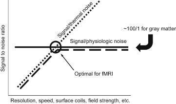
Figure 13 The signal to noise in fMRI time series. At low SNR values (left side of chart), thermal noise dominates, but at an SNR of approximately 100 to 1, physiologic noise, which also contains resting state fluctuations, starts to dominate. The dashed line is the time series SNR when collecting data from a living brain. Collecting EPI time series that have images with higher SNR than this physiologic noise limit does not add sensitivity. Therefore for fMRI, and in particular activation-based fMRI, it’s optimal to collect data at the elbow of this dashed curve—where physiologic noise is just starting to impose its limiting effect. If there were no physiologic noise, then the temporal signal to noise would continue to increase as the image signal to noise increases (dotted line).
Image Quality
The most prevalent image quality issues are image warping and signal dropout. While books can be written on this subject, the description here is kept to the essentials.
Because much of image quality has to do with magnetic field inhomogeneity, it’s useful to mention what is performed before each study to minimize this. Magnetic field “shimming” is a procedure in which current is adjusted through “shim” coils within the bore of the magnet that make small, spatially specific changes in the main magnetic field. This is a procedure in which specific areas where there is magnetic field inhomogeneity are targeted. The current in the shim coils is iteratively adjusted, typically using an algorithm rather than by hand, until the field inhomogeneities are reduced to a level that is satisfactory. That said, shimming is far from perfect, and field inhomogeneities still are prevalent, having a greater impact on image quality at higher field strengths and in particular on low-resolution, long readout-window sequences like EPI.
Image warping is fundamentally caused by three things: B0 field inhomogeneities; gradient nonlinearities; and in the case where extremely large gradients are applied such as with diffusion imaging, eddy currents. A nonlinear gradient will cause nonlinearities in spatial encoding, causing the image to be distorted. This is primarily a problem when using local, small gradient coils that have a small region of linearity that drops off rapidly at the edges of the field of view. With the prevalence of whole-body gradient-coils for performing echo planar imaging, this problem is not a major issue. If the B0 field is inhomogeneous, as is typically the situation with imperfect shimming procedures—particularly at higher field strengths, the protons will be processing at different frequencies than expected in their particular location. This will cause image deformation in these areas of poor shim—particularly with a long readout window or the long acquisition time of EPI. The long readout window duration allows for more time for these “off-resonance” effects to be manifest. Solutions to this include: obtaining a better B0 shim, mapping the B0 field to perform a correction based on this map, or, after the image has been reconstructed, performing image warping to match it with a non-warped high resolution structural image. Another viable solution is to reduce the readout window duration. This last solution is now possible with SMASH and SENSE imaging as this allows the same resolution image to be obtained in a fraction of the time, therefore producing images that suffer from much less warping.
Signal dropout is related to inhomogeneities in B0, typically at interfaces of tissues having different susceptibilities. If within a voxel, because of the B0 inhomogeneities, protons are precessing at different frequencies, their signals will cancel each other out. Several strategies exist for reducing this problem. One is, again, to shim as well as possible at the desired area. Due to imperfect shimming procedures, this solution helps but does not solve the signal dropout problem. The second potential solution is to reduce the voxel size (increase the resolution), thereby having less stratification of different frequencies within a voxel. The third potential solution is to choose the slice orientation such that the smallest voxel dimension (in many studies, the slice thickness is greater than the in-plane voxel dimension) is orientated perpendicular to the largest B0 gradient or in the direction of the greatest inhomogeneity.
Lastly, gradient electronics and structural improvements have mitigated eddy currents for most imaging applications. However, when the gradients are pushed extremely hard in the case of diffusion imaging, eddy currents that transiently exist can occur during the readout window, distorting the images. To make the problem worse, the distortions will depend on the directions in which the diffusion gradients are applied. In the case of diffusion tensor imaging, where gradients are applied in many different directions, distortions will occur in many different directions, causing the images to be out of alignment in many areas. Spatial correction procedures exist to mitigate these issues, but they are not perfect.
This brings up a final important point. A common operation is to superimpose a functional image, obtained with an EPI time series, on top of a structural image, obtained with multi-shot acquisition. Because these sequences have different readout window widths, they will have different amounts of distortion—particularly in areas of poor shim that have large off-resonance effects. There are two solutions. The first is to perform in post-processing a nonlinear image warping to better align the two images. This works for the most part; however, when attempting to align structure at the level of layers or columns, it tends to break down. The second solution is to use the EPI data for the structural underlay as well. For layer resolution work, this is essential as the EPI readout window is exceedingly long and the alignment has to be precise to less than about 0.1 mm. The general principle to take from this is that images with different readout window widths will have different levels of distortion that needs to be corrected if precise alignment is desired.
As with many of the topics discussed in this book, much more can be said, but the goal here is to introduce basic concepts and terms in a clear, practical way. MRI is a complex method that lies at the interface of engineering, physics, and human physiology. Development of all the technology mentioned in this chapter is still progressing—with improvements in speed, sensitivity, resolution, interpretability of the signal, and even the type of physiologic information obtained all coming about at a rapid rate.