Chapter 11
Spreadsheet-Based Concept Design and Examples

Having finished the outline constraint analysis, a more complete concept model can be constructed. Typically a finished concept design will be specified in around 100 numbers, of which perhaps 20 will relate directly to geometry – if greater detail is entered into, there is a danger that the design team will lose understanding of what parameters are controlling which aspects of the design. There does, however, need to be sufficient detail to enable simple sketches of the concept to be generated. The resulting design also needs to be balanced. Balance implies, for example, that lift is equal to weight (in level flight or a turn), available thrust is equal to drag (again in level flight or during takeoff or climb), the center of gravity lies close to the center of lift, and fuselage volume is sufficient for fuel, avionics, and payload, and so on, without being over-sized. Achieving balance almost always requires an iterative process to adjust key dimensions, something that can generally be specified in the form of an optimization problem and which can be set up and solved in a spreadsheet or similar environment. Constraint analysis provides the starting point for this process, enabling the design team to specify likely initial wing sizes and powerplant choices.

It is normal at the concept level to avoid using physics-based analysis codes to assess a design geometry, particularly during the iterative steps needed to balance the project. Rather, various design rules and equations will be invoked as in the previous chapter, see also, for example, the texts by Raymer [11] or Gudmundsson [15]. The problem with a physics-based approach is the need for more complete geometry data than is commonly available and the much longer calculation times involved. Research is progressing in this area but such tools tend to be limiting in the restrictions they impose on the design team. Thus CFD and FEA are not commonly used in concept design balancing work. They can, however, be invoked once a balanced design has been achieved to check whether the assumptions used in the design are still valid for the final concept. If they are not, assumptions can be adapted and a rebalancing carried out. It cannot be stressed too strongly that getting a design correctly balanced is of critical importance if the final product is to be satisfactory. It is clearly highly undesirable if the aircraft when finally built has an incorrect location of the center of gravity (CoG) and ballast has to be added – this might sound obvious but some quite major engineering projects have suffered because basic issues of balance and trim had not been dealt with correctly at the outset. When comparing configurations, it is again critical that all designs have been worked up properly into balanced possibilities to allow a fair decision. If it is intended to run more complex calculations, these should be completed and any subsequent rebalancing carried out before decisions are taken. In all cases, some measure of design merit will be needed to support the choices being made. This will have to take account of a range of possible performance and cost measures in some statement of overall value.

For the purposes of this chapter, we will begin with unmanned air vehicles (UAVs) with a dry take-off weight less than 40 kg. Initially, these will be taken to be powered by a single pusher propeller and piston engine system. Twin carbon tail booms and a U-shaped tail will be adopted. The fuselage can be nylon or glass-fiber-covered laser-cut foam with additional longitudinal stringers if desired. Reinforcement in laser-cut plywood or laser-sintered nylon will be possible. Molds and fiber layout will not be considered so as to reduce tooling and manpower costs. This information represents our topology and manufacturing choices and becomes embedded in the rules used to estimate weights for structural and fuselage components.

The designer starts with a given payload mass as well as landing and cruise speed combination (i.e., a design brief): here we begin with a payload of 2 kg, and landing, take-off, and cruise speeds of 15, 16, and 30 m/s, respectively. Maximum endurance is desired within an all-up maximum take-off weight (MTOW) – including payload and fuel – of 15 kg as used in the previous chapter.

The following sections set out the basic principles we use for sizing such a small, propeller-driven, piston-engine UAV. Most of the approaches we use are covered in Anderson [19] and Gudmundsson [15] with some additional data from Raymer [11], together with engine data sheets and propeller data sheets based on manufacturers' data and some results from our own experimental work. An extensive collection of independent propeller data can be found on the UIUC Propeller Data Site as compiled by John Brandt, Robert Deters, Gavin Ananda, and Michael Selig.¹ The Web-based program javaProp² can also be used to further check propeller behavior.

11.1 Concept Design Algorithm

The basic steps of the UAV platform concept design process used here are as follows:

1. Decide target payload mass, MTOW, and cruise speed (at a maximum cruise ceiling, for us typically 400 ft as set by UK CAA regulations) – we aim to maximize range within this MTOW budget and speed setting – other choices of start point are possible.

2. Choose the overall aircraft configuration (canard, monocoque, tail booms, etc.) – here taken as a tail boom pusher as already noted.

3. Choose the landing speed and take-off speed (or set take-off speed to be the same as landing speed), which govern wing loadings if we assume we do not have high lift devices – typical values are in the 12–18 m/s range. Higher landing speeds give faster, smaller aircraft with greater range but which are more likely to have accidents on landing!

4. Choose values for various fixed parameters – many of these are aerodynamic, all are nondimensional or do not depend on the airframe size and here are based on typical aircraft, operational speeds, previous designs and simple calculations (such as $c011-math-001$ , see, for example, Table 11.1.
5. Place some limits on what is possible or acceptable for the design under consideration – examples are given in Table 11.2.

6. To start the design process, choose the total main wing area from the constraint diagram along with likely coefficients of lift at cruise and landing (these are based on the chosen wing loading and the expected aerodynamic performance, including allowance for flaps or other landing aids if fitted), together with the fuel weight and longitudinal positions of tail-plane spar (to control static pitch stability) and payload (e.g., assumed to be forward of the front bulkhead and hence fixed by the location of this bulkhead) – ultimately we adjust these to balance the design and also ensure that they do not go outside the limits just set.

c011-math-002 — **Table 11.1** Typical fixed parameters in concept design.

c011-math-003 — **Table 11.1** Typical fixed parameters in concept design.

c011-math-011 — **Table 11.2** Typical limits on variables in concept design.

7. Choose the installed power needed from the constraint diagram or try and estimate the likely lift and drag of the aircraft at cruise, level turn, climb, takeoff, and landing for the given MTOW, so as to try and see what kind of installed power will be needed. If MTOW is fixed, this can be done without having to estimate the mass of the vehicle from its components, which is a distinct advantage of starting from a fixed MTOW.

8. Choose an engine/propeller combination and some likely dimensions for the aircraft fuselage (we set the datum on the center-line in way of the main wing spar, which is taken to lie at the quarter chord point). These dimensions can be used to sketch the aircraft; for the 15 kg Decode-1 aircraft used as the first example in this chapter, which has twin tail booms and conventional U-shaped rear control surfaces, they are as shown in Table 11.3. For other designs, they will need setting to different but appropriate values, based on prior experience or educated guesses.

c011-math-012 — **Table 11.3** Estimated secondary airframe dimensions.

c011-math-013 — **Table 11.3** Estimated secondary airframe dimensions.

9. Assess the likely empty weight based on the dimensions now available and the structural construction philosophy adopted, together with the components required to operate the aircraft (such as avionics, undercarriage, servos, and so on, that is, an outline list of component parts) plus the maximum fuel weight (without reserve). Ultimately MTOW includes
- payload weight
- structural weight
- avionics, systems, and servo weight
- propulsion system weight
- undercarriage and miscellaneous weight
- fuel weight including reserve.
When summing these, note that the dry weight does not include payload or the main fuel, but does include the fuel reserve.
10. Check if the following conditions have been met:
- the aircraft can rotate by at least the minimum angle specified at takeoff without fouling any part of the structure,
- the static margin is greater than the minimum required without being excessive,
- if a nose wheel is not fitted, the pitching moment caused by the propeller thrust and wheel drag (set equal and opposite to the thrust) will not cause the aircraft to pitch nose down into the ground, given the position of the CoG,
- there is enough weight difference between the MTOW, the structural weight, and the payload to carry some fuel!
- the wing $c011-math-015$ ratio at cruise is below the maximum chosen,
- the wing lift to total drag ratio at cruise is below the maximum chosen,
- the $c011-math-016$ at landing is below the permitted maximum,
- the installed static thrust is enough to start the aircraft rolling and to permit takeoff (assume that static thrust does not change until after the aircraft leaves the runway – in fact, it is likely to rise slightly for a well chosen propeller),
- the installed power is sufficient to achieve the cruise speed and to carry out acceptably banked level turns and climbs,
- the calculated aircraft weight including fuel is no more than the target MTOW (if it is less, more fuel is carried to simply increase the range),
11. Adjust the guessed inputs to maximize the range while meeting the constraints.

When this process is completed, the overall geometry of the balanced platform can then be used to begin the next stage of the design process. To carry out the above calculations, information is needed on a number of other aspects as described in the following sections.

11.2 Range

Range is given by the Breguet equation (for piston engined aircraft): $c011-math-017$ where SFC is in kg/kWh and the resulting range is in km. $c011-math-018$ is the propulsive efficiency at the cruise speed, typically around 0.6 but clearly varies with propeller choice and also speed. Note that here $c011-math-019$ does not include the fuel reserve.

11.3 Structural Loading Calculations

To size spars and booms, and hence estimate their weights, some form of maximum $c011-math-020$ to design against will be needed. This will come from gust or maneuver loads or some arbitrary choice such as $c011-math-021$ . Then simple beam theory can be used alongside design decisions on the likely form and materials to be selected for these items (typical materials are carbon-fiber tubes, solid or box-section plywood beams, or aluminum rods or tubes). Note that the FAA regulations (FARS 14, CFR, part 25) state that the maximum maneuver load factor is normally to be 2.5 but if the airplane weighs less than 50 000 lbs, the load factor is to be given by $c011-math-022$ , though $c011-math-023$ need not be greater than 3.8; while UK JAR 25 says: “the limit load maneuvering load factor $c011-math-024$ for any speed up to $c011-math-025$ may not be less than $c011-math-026$ except that $c011-math-027$ may not be less than 2.5 and need not be greater than 3.8, where $c011-math-028$ is the design MTOW.” Here the unit of weight is lbs. JAR-VLA (the equivalent standard for very light aircraft) simply says the limits should be between 1.5 and 3.8.

11.4 Weight and CoG Estimation

To estimate the total weight of the aircraft, a list must be made of all items carried (such as individual components of the avionics, including the wiring harness, undercarriage components, fuel tanks, servos, engine, etc.) and the locations of each item relative to the chosen datum noted, typically on a separate weights sheet (a relatively detailed example of a weights table is given in Chapter 15). For wing and fuselage structure, some construction method must be chosen and then estimates made using projected areas and lengths. Any spars or booms must be suitably sized with simple beam theory calculations as noted above. Monocoque areas subject to significant structural loads are difficult to estimate weights for accurately during concept sizing, but typically a surface area and thickness plus allowance for any rib stiffening has to suffice. Typical materials for stressed monocoques are carbon-fiber lay-up (possibly using foam sandwich techniques) or selective laser sintered (SLS) Nylon – in this chapter we restrict designs to SLS nylon or glass-fiber-covered hot-wire-cut foam. Tables 11.4 and 11.5 list some of the variables that might be used to scale weights and the items which might be scaled from them, respectively. Table 11.6 lists items whose weights are rather less easy to estimate, but which nonetheless may vary with aircraft size and must be allowed for.

c011-math-029 — **Table 11.4** Variables that might be used to estimate UAV weights

c011-math-030 — **Table 11.4** Variables that might be used to estimate UAV weights

c011-math-034 — **Table 11.5** Items for which weight estimates may be required and possible dependencies

Table 11.6 Other items for which weight estimates may be required

Item	Typical no. per a/c
R/C receiver	1
Batteries	2
Autopilot	2
Misc. avionics	1
Wiring and aerials	1
Engine covers	2
Main fuselage	0
Rear nacelle fuselage	2
Mid-wing skin & fuel tank	1
Rear wing box	1
Nose	2
Front bulkhead	2
Main undercarriage structure	2
Main wheels	2
Undercarriage mounting point	1
Catapult mounting	1
Tail undercarriage structure	2
Nose undercarriage structure	0
Tail wheels	2
Nose wheel	0

11.5 Longitudinal Stability

Static longitudinal (pitch) stability calculations are always needed, which require suitable downwash data for the elevator surfaces. Here we take the main wing quarter chord point as the datum and center of lift of the main wing:

$c011-math-035$

$c011-math-036$

where $c011-math-037$ is the longitudinal position of the center of gravity forward (positive) of the main wing quarter chord point, $c011-math-038$ is the longitudinal position of the tail-plane quarter chord behind (negative) the main wing quarter chord point. The value of 2 used twice is from theoretically perfect inviscid two-dimensional thin airfoil theory of 2 $c011-math-039$ for the lift curve slope – in practice, a value of 1.9 is more likely. The value of 3/4 used twice is the Oswald span efficiency and this is on the pessimistic side, 0.85 might be more likely. However, since both the perfect slope value and the span efficiency are applied to both wing and tail terms, the errors tend to cancel; if the main wing and tail-plane aspect ratios are equal they cancel completely. The terms essentially penalize low-aspect-ratio tail-planes slightly. Also in the downwash term $c011-math-040$ can be estimated from data provided in Raymer [11] (p. 482) and depends on wing aspect ratio (span $c011-math-041$ /area); wing semispan (assuming a rectangular wing); vertical position of tailplane compared to the main wing; longitudinal position of tail-plane quarter chord point behind wing quarter chord point; tail aspect ratio; $c011-math-042$ tail-plane longitudinal position/semi-span; $c011-math-043$ tail-plane vertical position/semispan. We leave consideration of dynamic stability until more detailed analysis is to take place, and instead rely on sensible tail volume coefficients to ensure a reasonable starting point has been chosen.

11.6 Powering and Propeller Sizing

By examining data from propeller manufacturers and their recommendations, it is possible to derive a simple regression curve that allows probable propeller diameter to be derived from engine capacity and likely pitch from diameter:

$c011-math-044$

$c011-math-045$

Also, one can estimate the likely engine capacity from engine power by looking at a range of small engines to get

$c011-math-046$ .

Then the (uncorrected) Abbott equations ³ link power, thrust, pitch, diameter, and rotational speed as:

$c011-math-047$

$c011-math-048$ .

Therefore, we can eliminate rpm to link thrust to power:

$c011-math-049$ .

So, given an engine power, we can estimate its likely static thrust when matched to a suitable propeller. Since we can also estimate the required thrust for cruise, banked turns, climb, and takeoff as described in the previous chapter, it is then possible to make an engine selection given the overall aircraft weight. For example, the estimated thrust needed for takeoff is given by

where the three terms represent the kinetic energy required during the ground roll, the mean aerodynamic drag on the runway, and the mean rolling resistance on the runway (recall that here $c011-math-050$ is the dynamic pressure at 70.71% of the take-off speed $c011-math-051$ ). The estimated thrust for climb is given by

where $c011-math-052$ is the vertical velocity in the climb and $c011-math-053$ is the lift-induced drag factor.

Next, using the UIUC Propeller Data Site,⁴ variations in propeller thrust with airspeed for a given diameter and rotational speed can be deduced by regressing plots of the thrust coefficient $c011-math-054$ versus the advance $c011-math-055$ . For example, for thin electric propellers with 12 in. pitch, the thrust coefficient can be approximated from the advance ratio as $c011-math-056$ . It is also possible, using JavaProp (and a suitable base propeller design operating at fixed torque), to calculate static thrust and to derive regression curves for thrust and required power as the forward velocity changes. In either case, these can be used to simulate runway roll-out and initial climb to check the results from the above equation and also to check whether the assumed propulsive efficiency is sensible. However, when the design is close to balance, we need to recognize that only existing engines can be specified and one should then switch to data for actual engines. Figure 5.3 given previously shows the powers and thrusts of typical UAV engine/propeller combinations.

11.7 Resulting Design: Decode-1

As part of the DECODE program mentioned in the introduction, we designed several aircraft adopting the principles set out in this book. The first of these, Decode-1, was a simple single-engine pusher aircraft that we used to gain information on performance and weights for subsequent design work. A pusher design was selected so as to give an uninterrupted view forward for the payload, but it does mean the fuselage length has to be sufficient to allow the payload mass to balance out the rear-mounted engine mass so as to yield an acceptable center of gravity. The aircraft was also designed to allow a range of different experimental wings to be trialed and was sized so as to fit inside our largest wind tunnel without significant modification. Figures 11.1 and 11.2 show this aircraft with conventional wings attached.

Photo of Decode-1 in the R.J. — **Figure 11.1** Decode-1 in the R.J. Mitchell wind tunnel with wheels and wing tips removed and electric motor for propeller drive.

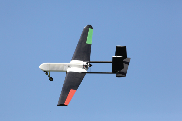
Photo of Decode-1 in flight with nose camera fitted. — **Figure 11.2** Decode-1 in flight with nose camera fitted.

The basic design brief for the aircraft is given in Table 11.7. If this brief, together with the data from Tables 11.1–11.3, is fed into our spreadsheet system, which follows the algorithm previously outlined, the design details given in Tables 11.8 and 11.9 result; see also Figures 11.3–11.5, which show the inputs, results, and simplified layout sketches we create inside the spreadsheet during design studies⁵. We find that seeing the aircraft in planform and side view in this way is very helpful when making design judgments early on in the design process; it is immediately apparent how similar this is to the layout of the final aircraft.

Table 11.7 Design brief for Decode-1

Item	Value	Units
Payload mass	2	kg
Maximum take-off weight set by design	15	kg
Maximum cruise speed	30	m/s
Landing speed	15	m/s
Take-off speed	16	m/s
Length of ground roll on take-off	60	m
Runway altitude	0	m
Cruising height	121.92	m

c011-math-057 — **Table 11.8** Resulting concept design from spreadsheet analysis for Decode-1

c011-math-058 — **Table 11.8** Resulting concept design from spreadsheet analysis for Decode-1

The first five entries here are manipulated by the solver tool within the spreadsheet to maximize the range.

Table 11.9 Design geometry from spreadsheet analysis for Decode-1 (in units of mm and to be read in conjunction with Tables 11.3 and 11.8)

Item	Value
Total wing span (rect. wing)	2948.3
Aerodynamic mean chord	327.6
Propeller diameter	435.0
Tail-plane span	797.4
Tail-plane mean chord	199.3
Fin height (or semi-span) for two fins	293.0
Fin mean chord	195.3
Long position of middle bulkhead	220.0
Horizontal position of tail booms	239.2

Note that three of the constraints set out in Table 11.2 are actively limiting the design: the peak wing $c011-math-063$ at cruise speed is 16; the allowable rotation at takeoff before grounding happens is 17°; and the static margin (expressed in fractions of main wing chord) is 0.1. Of these, it is the $c011-math-064$ value that is most fundamental aerodynamically, the other two largely dictating the fuselage and tail-boom length. The maximum value of $c011-math-065$ is set by the wing technology being deployed and depends on the detailed choice of planform, sections, twist, and wing tip treatment. The value of 16 used here is intimately related to the wing loading discussed in the previous chapter, and for operations at sea level and 30 m/s gives a wing loading of 15.5 kg/m $c011-math-066$ . The value of $c011-math-067$ used is something we know we can achieve in practice using the construction methods we have adopted; higher values are possible but these tend to make the wings more difficult and expensive to make. For example, we chose to taper our wings linearly and avoid twist when working with hot-wire-cut foam; twisted or elliptic planform wings would give better control of induced drag, but instead we often make use of quite sophisticated 3D-printed wing tips to limit induced drag, see again Figure 11.2.

Once one is happy that the concept is sufficiently well developed to warrant further effort, the basic geometry details can then be used to generate a more realistic and fully three-dimensional outer envelope for the aircraft. To do this, we use the AirCONICS suite of programs,⁶ which leads to the design shown in Figure 11.6. This can then be used for further analysis or to start the process of building a detailed CAD model suitable for generating manufacturing drawings. Note that the AirCONICS geometry includes wing taper, an aerodynamically shaped circular fuselage, faired in-tail booms, and slab-sided undercarriage legs. These are just working assumptions at this stage, but the resulting model is sufficiently detailed for reasonable CFD and FEA analysis. No attempt at this stage has been made to add control surfaces to the wings, tail, or fins, so any CFD results would be solely for the cruise configuration. These can be added later using AirCONICS, as will be seen in Chapter 13. The final design shown in Figure 11.2 has greater wing taper, wing tips, and a triangular section fuselage, but otherwise is broadly similar to this initial AirCONICS model.

Illustration of Decode-1 spreadsheet snapshot - inputs page. — **Figure 11.3** Decode-1 spreadsheet snapshot – inputs page.

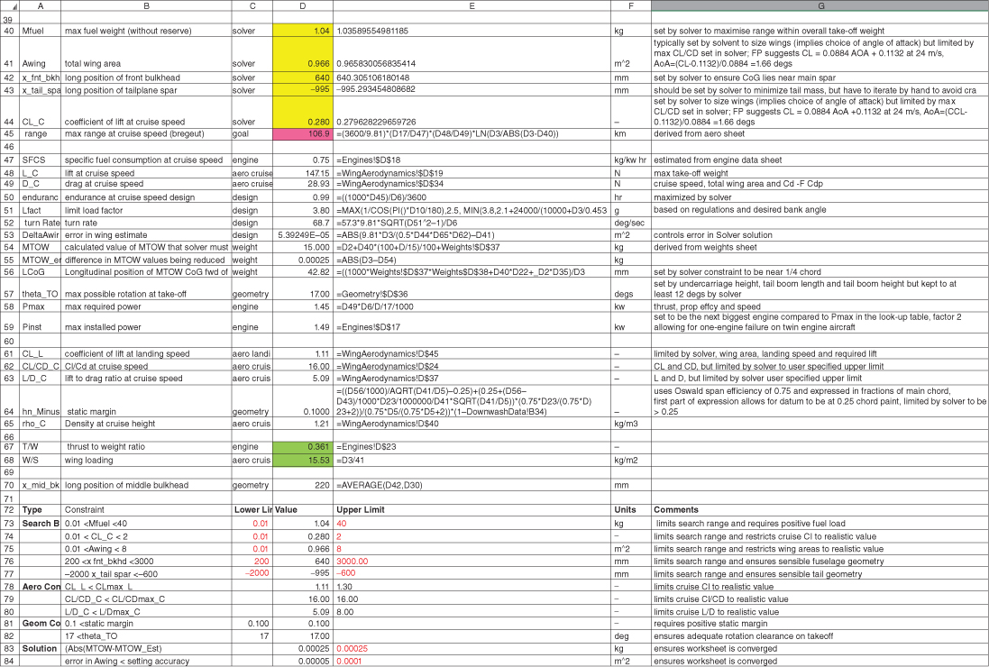
Illustration of Decode-1 spreadsheet snapshot - results summary page. — **Figure 11.4** Decode-1 spreadsheet snapshot – results summary page.

Illustration of Decode-1 spreadsheet snapshot - geometry page.

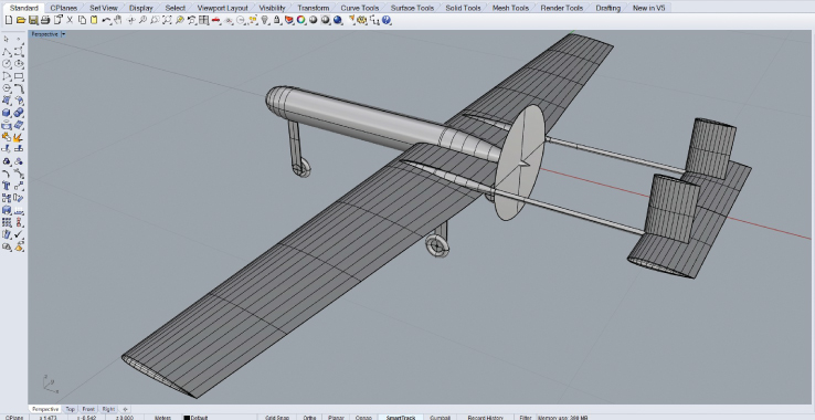
Snapshot of Decode-1 outer geometry as generated with the AirCONICS tool suite. — **Figure 11.6** Decode-1 outer geometry as generated with the AirCONICS tool suite.

11.8 A Bigger Single Engine Design: Decode-2

The next aircraft we consider is an enlarged variant of Decode-1 that has 50% greater payload capability and endurance, a larger margin on installed power (a shorter ground roll is specified), and usefully lower landing speed, all made possible by the use of an inverted V tail and large flaps. The inverted V tail is allowed in the design process by reducing the tail volume coefficients needed by 30%, which gives a smaller, lighter tail and easier control of the static margin. The flaps allow a greater lift coefficient in the landing configuration and hence lower approach speed. Decode-2 is also a single pusher design with a nose-mounted camera system. The design brief is set out in Table 11.10 and the secondary dimensions in Table 11.11. The wing loading is slightly lower (this is now controlled by the choice of maximum landing $c011-math-068$ of 1.55) but a slightly less stringent rotation at takeoff of 14° is chosen. The other parameters given in Table 11.2 are held fixed as before.

Table 11.10 Design brief for Decode-2

Item	Value	Units
Payload mass	3	kg
Maximum take-off weight set by design	23.5	kg
Maximum cruise speed	30	m/s
Landing speed	12.5	m/s
Take-off speed	16	m/s
Length of ground roll on take-off	45	m
Runway altitude	0	m
Cruising height	121.92	m

c011-math-069 — **Table 11.11** Estimated secondary airframe dimensions for Decode-2

c011-math-070 — **Table 11.11** Estimated secondary airframe dimensions for Decode-2

c011-math-072 — **Table 11.12** Resulting concept design from spreadsheet analysis for Decode-2

c011-math-073 — **Table 11.12** Resulting concept design from spreadsheet analysis for Decode-2

The first five entries here are manipulated by the solver tool within the spreadsheet to maximize the range.

The resulting design is detailed in Tables 11.12 and 11.13 along with the screenshot in Figure 11.7. The aircraft is shown in flight in Figure 11.8 and the outer shape modeled with AirCONICS in Figure 11.9. Note that our spreadsheet sketch does not distinguish between an H and an inverted V tail (simple horizontal and vertical projections being provided); this level of detail has to be worked up after the initial spreadsheet-based concept has been defined, which is straightforward to create within AirCONICS.

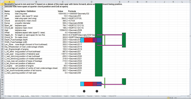
Illustration of Decode-2 spreadsheet snapshot. — **Figure 11.7** Decode-2 spreadsheet snapshot.

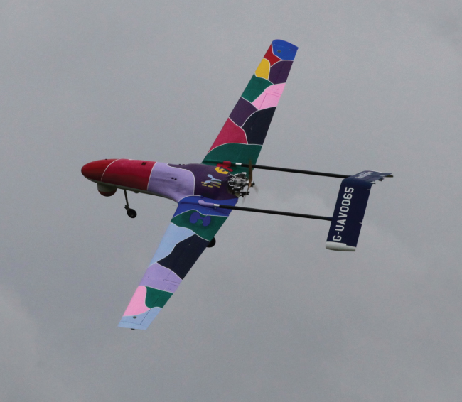
Illustration of Decode-2 in flight with nose camera fitted. — **Figure 11.8** Decode-2 in flight with nose camera fitted.

Table 11.13 Design geometry from spreadsheet analysis for Decode-2 (in units of mm and to be read in conjunction with Tables 11.11 and 11.12)

Item	Value
Total wing span (rect. wing)	3942.2
Aerodynamic mean chord	394.2
Propeller diameter	550.4
Tail-plane span	784.7
Tail-plane mean chord	196.2
Fin height (or semi-span) for two fins	303.9
Fin mean chord	202.6
Long position of middle bulkhead	218.9
Horizontal position of tail booms	302.7

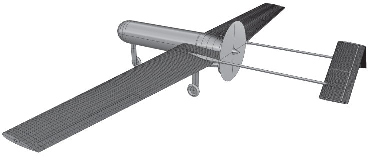
Outline for Decode-2 outer geometry as generated with the AirCONICS tool suite. — **Figure 11.9** Decode-2 outer geometry as generated with the AirCONICS tool suite.

11.9 A Twin Tractor Design: SPOTTER

Our third example is the twin tractor aircraft SPOTTER. This is bigger again and is designed to have a high level of redundancy to ensure better operational resilience. The aircraft is designed to carry an interchangeable underslung payload pod of up to 5 kg weight and makes use of an integral fuel tank. It carries dual on-board charging systems powered from the main engines. The design brief is set out in Table 11.14 and the estimated secondary dimensions in Table 11.15. The wing loading is now slightly lower (this is again controlled by the choice of maximum landing $c011-math-078$ of 1.55), and a rotation at takeoff of 15° is used. The other parameters given in Table 11.2 are held fixed as before. Here the engines are sized so as to be able to maintain flight with one engine nonoperational but not so as to be able to complete a take-off run with only one engine with full fuel and payload. The resulting design is detailed in Tables 11.16 and 11.17 along with the screenshot in Figure 11.10. The aircraft is shown in flight in Figure 11.11 and the outer shape modeled with AirCONICS in Figure 11.12.

Table 11.14 Design brief for SPOTTER

Item	Value	Units
Payload mass	5	kg
Maximum take-off weight set by design	30	kg
Maximum cruise speed	30	m/s
Landing speed	12.5	m/s
Take-off speed	16	m/s
Length of ground roll on takeoff	60	m
Runway altitude	0	m
Cruising height	121.92	m

c011-math-079 — **Table 11.15** Estimated secondary airframe dimensions for SPOTTER

c011-math-080 — **Table 11.16** Resulting concept design from spreadsheet analysis for SPOTTER

c011-math-081 — **Table 11.16** Resulting concept design from spreadsheet analysis for SPOTTER

The first five entries here are manipulated by the solver tool within the spreadsheet to maximize the range.

Table 11.17 Design geometry from spreadsheet analysis for SPOTTER (in units of mm and to be read in conjunction with Tables 11.15 and 11.16)

Item	Value
Total wing span (rect. wing)	4196.3
Aerodynamic mean chord	466.3
Propeller diameter	493.6
Tail-plane span	1154.1
Tail-plane mean chord	288.5
Fin height (or semispan) for two fins	424.1
Fin mean chord	282.7
Long position of middle bulkhead	165.0
Horizontal position of tail booms	271.5

Illustration of SPOTTER spreadsheet snapshot. — **Figure 11.10** SPOTTER spreadsheet snapshot.

Photo of SPOTTER in flight with payload pod fitted. — **Figure 11.11** SPOTTER in flight with payload pod fitted.

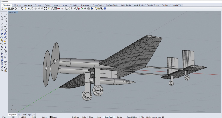
Illustration of SPOTTER outer geometry as generated with the AirCONICS tool suite. — **Figure 11.12** SPOTTER outer geometry as generated with the AirCONICS tool suite.

Item	Value
Aspect ratio (span $c011-math-002$ /area)	9
Reserve fuel fraction	0.1
Minimum (wing) coefficient of drag at cruise speed, $c011-math-003$	0.0143
Viscous drag constant, $c011-math-004$	0.0329
Pressure and induced drag constant, $c011-math-005$	0.0334
Minimum drag (wing) coefficient of lift at cruise speed, $c011-math-006$	0.1485
Coefficient of parasitic drag at cruise speed	0.0375
$c011-math-007$ at landing speed	5
Coefficient of parasitic drag at landing speed	0.05
$c011-math-008$ at take-off speed	5
Coefficient of parasitic drag at take-off speed	0.035
Equivalent rolling coefficient of friction	0.225
Propulsive efficiency at cruise speed	0.6
Tail-plane aspect ratio (span $c011-math-009$ /area)	4
Fin aspect ratio, ((twice fin height) $c011-math-010$ /area) assuming two fins	3
Bank angle in level turn	60°
Minimum rate of climb from cruise	5m/s
Percentage extra thrust desired to start ground roll	0%

Name	Long name/definition	Typical value	Unit
Awing	Total wing area	1.54	m $c011-math-029$
AR	Aspect ratio (spanˆ2/area)	9.00	—
Thick	Aerodynamic mean thickness	62.1	mm
Atail	Tailplane area	226 222	mm $c011-math-030$
Afin	Fin area	203 600	mm $c011-math-031$
y_ tail_ boom	Horizontal position of tail booms	271.5	mm
Span_ tail	Tailplane span	951.3	mm
Chord_ tail	Tailplane mean chord	237.8	mm
Height_ fin	Fin height (or semispan) for two fins	390.8	mm
Chord_ fin	Fin mean chord	260.5	mm
Vmax_ C	Maximum cruise speed	30.0	m/s
x_ main_ spar	Long position of main spar	0.0	mm
x_ fnt_ bkhd	Long position of front bulkhead	240.3	mm
x_ tail_ spar	Long position of tailplane spar	$c011-math-032$	mm
x_ rear_ bkhd	Long position of rear bulkhead	$c011-math-033$	mm
x_ mid_ bkhd	Long position of middle bulkhead	20.2	mm
Depth_ Fuse	Fuselage depth	250	mm
Width_ Fuse	Fuselage width	190	mm
Len_ Nose	Nose length (forward of front bulkhead)	200	mm
Len_ Engine	Length of engine	125	mm
Mengine	Engine mass	2.072	kg
Dprop	Propeller diameter	494	mm
DTop	Design topology	3	—

Item	Typical no. per a/c	Possible dependency
Wing spars (incl. center spars)	2	Wing area, spar length, speed
Wing ribs $c011-math-034$ nylon parts	6	Wing cross-sectional area
Wing foam	2	Wing box volume
Wing covers	4	Wing area
Ailerons	2	Wing box volume
Flaps	2	Wing box volume
Tail boom	2	Tail-plane area, spar length, speed
Tail fin	2	Individual fin area
Tailplane	1	Tail-plane area
Rudder	2	Individual fin area
Elevators	1	Tail-plane area
Engine	2	List of engine weights
Muffler	2	List of engine weights
Propeller	2	Prop dia.
Generator	2	Engine mass/?fixed
Ignition unit	2	Engine mass/?fixed
Fuel tank	0	Engine mass/?fixed
Aileron servos	2	Wing area
Flap servos	0	Wing area
Throttle servo	1	Engine mass/?fixed
Rudder servo	2	Individual fin area
Elevator servo	1	Tail-plane area
Wheel steering servo	2	Wing area
Linkages and bell-cranks	8	Total wing area/?fixed

Item	Value	Units
Maximum fuel weight (without reserve)	1.04	kg
Total wing area	0.966	m $c011-math-057$
Long position of front bulkhead	640	mm
Long position of tail-plane spar	$c011-math-058$	mm
Coefficient of lift at cruise speed	0.280	—
Maximum range at cruise speed (Breguet)	106.9	km
Lift at cruise speed	147.15	N
Drag at cruise speed	28.93	N
Endurance at cruise speed	60.0	min
Limit load factor	3.80	g
Turn rate	68.7	$c011-math-059$ /s
Longitudinal position of MTOW CoG fwd of main spar	42.8	mm
Maximum possible rotation at takeoff	17.0	$c011-math-060$
Engine selected	OS Gemini FT-160	—
Specific fuel consumption at cruise speed	0.75	kg/kWh
Maximum required power	1.45	kW
Maximum installed power	1.49	kW
Coefficient of lift at landing speed	1.11	—
Wing $c011-math-061$ at cruise speed	16.0	—
Lift to drag ratio at cruise speed	5.09	—
Static margin	0.10	—
Thrust to weight ratio	0.361	—
Wing loading	15.53	kg/m $c011-math-062$

Item	Value	Units
Fuselage depth	225	mm
Fuselage width	250	mm
Nose length (forward of front bulkhead)	200	mm
Diameter of main undercarriage wheels	125	mm
Longitudinal position of engine bulkhead	$c011-math-069$	mm
Vertical position of base of fuselage	$c011-math-070$	mm
Vertical position of tail-plane	0.0	mm
Vertical position of engine	60	mm
Vertical position of center of main undercarriage wheels	$c011-math-071$	mm

Item	Value
Maximum wing $c011-math-011$ at cruise speed	16
Maximum wing lift to total drag at cruise speed (allows for all drag elements)	8
Maximum coefficient of lift at landing speed	1.3
Minimum allowable rotation at take-off before grounding happens	17°
Minimum static margin (expressed in fractions of main wing chord)	0.1