From Neutrons to Life: A Complex Trinity
As West and East
In all flatt Maps—and I am one—are one,
So death doth touch the Resurrection.
—John Donne, “Hymn to God, My God, in My Sickness”
On July 16, 1945, the atomic age began. At just past 5:29 a.m. Mountain War Time, in the remote Jornada del Muerto basin (a desert in southern New Mexico aptly named by Spanish conquistadors for its “single day’s journey of the dead man”), the Manhattan Project tested an implosion-initiated plutonium device that released the equivalent of around twenty kilotons of TNT. The test, conducted under the auspices of the project’s scientific leader, J. Robert Oppenheimer, was code-named Trinity, apparently derived from Oppenheimer’s reading of two John Donne poems: “Hymn to God,” which opens this chapter, and “Batter my heart, three person’d God.” Three weeks later, an atomic bomb based on an untested but simpler design using uranium-235 was dropped on Hiroshima, Japan. Three days after that, a device based on the Trinity design was dropped on Nagasaki. Shortly thereafter, Japan surrendered, ending World War II.
Nuclear reactions, whether used for civilian power or for nuclear bombs, rely on interactions. In one type of reaction, energetic neutrons potentially collide with nearby nuclei, perhaps resulting in a fission event that releases some energy and even more energetic neutrons into the mix. Note the use of the words “potentially” and “perhaps.” Chance plays an important role in such systems. If neutrons beget neutrons, there is the potential to transform mass into energy à la Einstein’s famous E = mc2. Depending on the speed of that transformation, we can get either warming leading to the carbon-free generation of civilian power or the destructive force of a nuclear blast. Given the potential energy inherent in an atom, it is not surprising that at the start of the war there was an intense interest in understanding the complex interactions that take place at this atomic scale. Such interactions embody the first branch of a complex trinity that leads us to a fundamental theorem about complex adaptive systems.
The second branch of our trinity begins with a decision to build a secret new device called the Electronic Numerical Integrator and Computer at the University of Pennsylvania’s Moore School of Electrical Engineering. Called the ENIAC, it was the first programmable electronic computer, and it was a milestone development in the information age. The initial proposal to build ENIAC was made to the United States Army’s Ballistics Research Laboratory at Aberdeen Proving Ground in Maryland by the physicist John Mauchly. Mauchly was inspired to find a better way to generate ballistic firing tables after encountering a group of women—known at the time as “computers”—literally cranking out such tables on desk calculators. Mauchly and an engineer, Presper Eckert, took charge of the ENIAC program, resulting in the eventual development of a thirty-ton electronic computer requiring 1,800 square feet of floor space, 17,500 vacuum tubes, and an astounding number of solder joints.
John von Neumann was a consultant to Aberdeen. Upon learning about ENIAC, he realized that it might be repurposed to help solve the “thermonuclear problem”—that is, a bomb predicated on nuclear fusion rather than fission—being pursued by some of von Neumann’s Los Alamos colleagues led by physicist Edward Teller. In March 1945, von Neumann, Nick Metropolis, and Stan Frankel visited the Moore School and began to finalize plans for building a computational model of a thermonuclear reaction that would be run on ENIAC.
While the war ended before they had completed their work, by the spring of 1946 Metropolis and Frankel had discussed ENIAC with and presented their calculations and conclusions to a high-level group in Los Alamos, including von Neumann, Teller, Los Alamos director Norris Bradbury, Enrico Fermi, and Stan Ulam. Although the model was simple, the results were encouraging. In the annals of complex systems, this represents an important milestone in the use of electronic computation to understand complex interactions with serious, real-world implications.
Inspired by the results of Metropolis and Frankel, Ulam realized that a number of cumbersome but powerful statistical sampling techniques could be implemented using electronic computers. Ulam discussed this idea with von Neumann, who broached it with the leader of the Los Alamos Theoretical Division. The approach used computationally generated randomness to solve complex problems, and it marks the formal beginning of what has come to be known as the Monte Carlo method.a (The name was suggested by Metropolis, and it was “not unrelated to the fact that Stan [Ulam] had an uncle who would borrow money from relatives because he ‘just had to go to Monte Carlo.’”) By the late 1940s the Monte Carlo method, promoted by various symposia, had become an accepted scientific tool.
Monte Carlo methods played a key role in a groundbreaking paper, “Equation of State Calculations by Fast Computing Machines,” published in 1953. The paper had five authors: Metropolis, Arianna and Marshall Rosenbluth, and Augusta and Edward Teller. At the heart of the paper was “a general method, suitable for fast electronic computing machines, of calculating the properties of any substance which may be considered as composed of interacting individual molecules.” This has become known as the Metropolis algorithm.
The paper focused on the question of how interacting particles will be distributed in space. Each particle interacts with the others, and we can calculate the overall energy for any given configuration. The challenge posed in the paper was to find the most likely configurations for this system.
One approach to solving this problem would be to model particles as coins and space as a tabletop. We could randomly toss coins on the table, calculate the energy of the resulting configuration as if the coins represented the position of atoms, and repeat. After numerous repetitions, we would begin to get a sense of the distribution of possible energy states for the system. Alas, the problem with this approach is that a lot of our effort will be spent on generating configurations that are not all that likely to appear. In physics, it is assumed that systems seek out lower-energy configurations, and a lot of our random tosses would result in high-energy configurations that we are not likely to observe.
Metropolis and colleagues provided an alternative solution for finding the most-likely configurations, and the technique embodied in this solution has profound implications both for modern statistical methods and, as we will see in the last branch of our trinity, for understanding complex adaptive systems.
The solution suggested by Metropolis and his coauthors seems remarkably simple on its face. First, begin with a randomly derived configuration of the coins and label this the status quo. Next, consider a new configuration of the coins generated by taking the status quo and randomly moving one of the coins by a small amount using a random process driven by a proposal distribution. We now calculate some measure of interest tied to the resulting configurations (in the above system, the amount of energy resulting from the interactions of atoms tied to the locations of the coins) for both the status quo and the new configuration. We then use an acceptance function to decide which of these two configurations will become the new status quo. If the candidate configuration is superior to the previous status quo, the candidate is accepted immediately as the new status quo. If the candidate configuration is inferior, then the likelihood that it replaces the previous status quo is proportional to their respective measures of interest. The more inferior the candidate is to the previous status quo, the less likely it will become the new status quo.
The algorithm proceeds by iterating the steps above using the current status quo. Amazingly, if we track the various configurations that this algorithm visits over time, we find that these configurations converge on the exact distribution underlying the measure of interest. That is, the system will spend relatively more time in those configurations that have the highest measure of interest. In the case of our particle system above, if we run the algorithm for a while and then randomly sample the status quo, we will tend to find the system in low-energy states.
Intuitively, the algorithm’s behavior makes sense, as our acceptance criteria tend to direct the system into areas with higher measures of interest while avoiding areas with lower values. That being said, the fact that the system perfectly aligns with the distribution tied to the measure of interest is much more surprising, given that the algorithm never uses any global information about the underlying distribution.
However miraculous the algorithm’s behavior may seem, it is possible to understand it mathematically. The first key piece is that the algorithm always uses the existing status quo as an anchor. The status quo embodies some important information, and thus the algorithm is not just randomly searching across possible configurations, which would result in a very different outcome. For example, we can forecast the weather by simply calculating the number of days that it rains throughout the year and then using this proportion as our prediction of rain on any given day. Alternatively, we could calculate the likelihood of rain on a particular day given that it rained on the previous day. As you might suspect, the latter approach gives us a very different set of probabilities and, in the case of weather, a much more accurate prediction, since the weather today is a good predictor of the weather tomorrow.
The idea that one event—say, yesterday’s weather or the status quo configuration—might influence the probability of the next event goes back to the Russian mathematician Andrey Andreyevich Markov in the early 1900s, who developed a number of important results about these systems that are now known as Markov chains. The 1953 paper of Metropolis and colleagues used some of Markov’s ideas to create a new class of algorithms called Markov chain Monte Carlo (MCMC) methods.
If the probabilities that govern the transitions from one state to another make it possible to go from every state to every other state (though not necessarily in one move), then the Markov chain is known as ergotic (or irreducible). If such transitions are always possible after n or more steps, the chain is called regular.b In the MCMC algorithm, it is easy to choose a proposal distribution for the next configuration that will guarantee that the resulting Markov chain will be regular. Typically, it also is useful to have a symmetric proposal distribution (as was done in the original Metropolis algorithm). This requires that the probability of proposing x given y is identical to the probability of proposing y given x.
The fact that MCMC algorithms are driven by a regular Markov chain is useful, as these chains become increasingly well behaved as the system runs forward. Such systems collapse into a very well-behaved regime where the probability of finding it in any particular state is fixed and independent of where the system started. That is, if we run our MCMC algorithm long enough, the system will start to visit the various states in a predictable way. In the case of weather, regardless of the weather today, if we wait long enough, the chance of rain on a randomly chosen day in the future will be fixed. These systems do, however, require a certain amount of burn-in time. While we can start the system anywhere, it takes the chain a certain amount of time to forget where it began and to find its more fundamental behavior. Exactly how long that takes has important implications for adaptation.
The second key aspect of the MCMC’s remarkable behavior involves the acceptance criteria. The choice of the acceptance criteria is made with careful forethought, as it guarantees that the algorithm converges to the underlying probability distribution implied by our measure of interest. The odd thing about this convergence is that we typically cannot calculate this probability distribution directly, as it requires information about all possible configurations of the system, and the number of such configurations is usually so large that performing this calculation is impossible. Fortunately, the algorithm doesn’t need to directly perform such a calculation. A sufficient condition that guarantees the needed convergence is a property known as detailed balance. Detailed balance requires that when the system converges, the resulting transitions are reversible in the sense that the equilibrium probability of moving from one configuration to another is the same in either direction. If detailed balance holds, then the system converges to the underlying probability distribution driving the measure of interest.
Arthur C. Clarke noted that “any sufficiently advanced technology is indistinguishable from magic,” and perhaps MCMC is one such technology. Through a very simple set of manipulations—randomly creating a candidate configuration contingent on the status quo and possibly replacing the status quo with that candidate configuration based on a roll of the dice tied to the relative measures of interest of the two configurations—we create a system that is driven by a much deeper force, one that was previously inaccessible to us given the impossibility of making the required calculations. MCMC methods have radically altered the scientific landscape. In particular, such algorithms are needed for the widespread application of Bayesian statistics, a now ubiquitous approach that is ushering in a new analytic age characterized by everything from targeted web ads to driverless cars. At the heart of Bayesian methods is the need to calculate some key probability distributions. Such distributions are often computationally impossible to calculate directly, but we can invoke the magic of MCMC.
This brings us to the third branch of our complex trinity, namely, the implications of the first two branches for understanding complex adaptive systems. The impetus for the original development of MCMC algorithms was to find a simple method that could reveal a previously hidden but vitally important distribution. In the case of Metropolis and colleagues, this was the distribution of the likely energy states for a system of interacting particles. To accomplish this goal, the creators of the algorithm developed a set of simple, iterative steps that generated the needed candidates. As if by magic, such simple steps are sufficient to uncover the desired distribution. The implications of MCMC algorithms are even more profound for complex adaptive systems. The mechanisms that drive adaptive systems, such as evolution, have direct analogs to the key elements of the MCMC algorithm. In short, a complex adaptive system behaves as if it were implementing a MCMC algorithm.
Consider a pond covered with lily pads, on one of which sits a frog. We assume that each lily pad, depending on its location, has some inherent value for the frog—say, the number of flying insects that the frog can snatch in a given time (assuming that the supply of such insects is constantly renewed). Suppose the frog behaves as follows: Every minute it randomly picks a neighboring lily pad, and if the number of insects at that new pad is greater than the number at the current pad, it jumps to the neighboring pad. Otherwise, it jumps to the new pad with a probability proportionate to the relative number of insects at the two locations. Thus the chance of moving will be higher the closer the number of insects at the neighboring pad is to the number at the current one.
As might be apparent, the frog is in the midst of a MCMC algorithm. The lily pads represent various states of the system, and the location of the frog marks the status quo configuration. When the frog considers a randomly chosen neighboring lily pad, it is drawing from a proposal distribution. The frog’s decision to jump to the new pad (that is, to create a new status quo) is implemented via the acceptance criteria used in the Metropolis algorithm, always accepting the new pad (state) if it is better, and if it is worse, accepting it with a probability tied to the relative quality.
Given that the frog is implementing a MCMC algorithm, we can easily characterize its long-run behavior. After a certain amount of initial hopping (aka burn-in time), if we track the frog’s location, we will find that the amount of time it spends on any particular lily pad is given by the number of insects found at that pad divided by the total number of insects across all of the pads. These fractions, taken together, give us a probability distribution describing the likelihood of the frog being on a particular lily pad sometime in the future. For example, if we have three lily pads, the first one with fifty insects, the second one with thirty, and the third one with twenty, then over time the frog will be on the first pad 50 percent of the time, on the second one 30 percent of the time, and on the third one 20 percent of the time (see Figure 12.1).
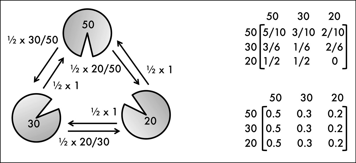
Figure 12.1: Three lily pads with different numbers of flying insects given by the numeric label in each pad. We assume that at each time step the frog has an equal chance of picking one of the two neighboring lily pads and moving to it based on the Metropolis acceptance criteria. The diagram on the left illustrates the overall design, with the labeled arcs providing the probability of choosing that neighbor (½ in all cases) × the acceptance probability. The top matrix on the right gives the transition probabilities for the resulting Markov chain Monte Carlo process, that is, the probability of moving to the pad designated by the column, given that you are currently on the pad designated by the row. After many time steps, the system converges to the bottom transition matrix, with the frog residing on the 50-, 30-, and 20-insect lily pads 50 percent, 30 percent, and 20 percent of the time, respectively. This bottom matrix is the result of repeatedly multiplying the top matrix by itself.
What’s true for frogs and ponds can also be true for other adaptive systems. Configurations of an agent in an adaptive system represent various states of the system. An agent pursues goals by reconfiguring itself in constrained ways and moving toward new configurations that result in better outcomes. So if we are willing to make some key simplifications of reality, we can generate a useful model of an adaptive agent in a complex system and use MCMC ideas to derive a fundamental theorem about this system’s behavior.
To begin this process, we need to think about how an agent represents various states. In biology, for example, an organism’s genotype represents a possible state of the system of all genotypes. In economics, states can represent, say, the standard operating procedures of a firm, the design of a product, the consumption bundle of a consumer, or some rule of behavior. In a city, states could represent the network of roads or the locations of activities.
Given the state space of an adaptive system, the MCMC approach requires a notion of identifying new possible states using a proposal distribution. For a well-behaved MCMC, the requirements for the form of the proposal distribution are relatively light—not much more than some reasonable ability to move, eventually, from one state to another. (For convenience, we might want to impose some more restrictions, such as requiring that this distribution be symmetric.) In adaptive systems, the notion that existing structures can be randomly altered by a mutation-like operator tends to be an easy assumption to embrace and one that meets the above requirements. Indeed, mutation is central to biological systems, and it also approximates the behavior observed in a variety of other systems. For example, new products are often slight variants of old ones, new technological or scientific ideas rest on the shoulders of giants, consumers make slight alterations in the goods that they buy, and so on.
The algorithm needs a measure of fitness for any given state of the system. For our frog, insects serve as this measure, as presumably the more insects the frog consumes, the happier it is. Similar measures of fitness arise in other adaptive systems. For example, in biology there is a notion of fitness that is tied not only to the food supply but also to the overall ability of an organism to survive and reproduce. In economics, we often think of agents pursuing profit (in the case of firms) or happiness (in the case of consumers). Thus, as long as agents in an adaptive system are pursuing a goal, we can use the measure of this goal as a means to drive our model.
Finally, our model requires that the adaptive system adopt the proposed variant based on a MCMC-compatible acceptance criteria. The criteria developed by Metropolis and his coworkers always accepted any variant that had higher fitness than the status quo, and when the fitness of that variant was less than that of the status quo, the criteria adopted it probabilistically, with the likelihood diminishing as the difference in fitness between the two options increased. Such a rule seems to be a reasonable approximation for many adaptive systems.
There may be other acceptance criteria that will also result in detailed balance and thereby provide the needed convergence. For example, if the proposal distribution is symmetric, an acceptance criterion that adopts the variant with a probability given by the variant’s fitness divided by the fitness of both the variant and the status quo also results in detailed balance. Under such a rule, if the value of the variant is equal to that of the status quo, there is a 50 percent chance that it is adopted, and as the variant’s value rises (falls) the adoption probability increases (decreases) away from 50 percent. (By the way, all is not lost if the system has acceptance criteria without detailed balance, as it will still converge to a unique distribution, but that distribution will differ from the one specified below, though perhaps only slightly.)
Suppose we have an adaptive system where an agent represents a possible state of the system. At each time step, a reasonable variant of this agent is tested against the environment, and that variant replaces the existing agent based on detailed-balance-compatible acceptance criteria tied to relative fitness. This leads to a fundamental theorem of complex adaptive systems: in the above adaptive system, after sufficient burn-in time, the distribution of the agent (states) in the system is given by the normalized fitness distribution.
The proof of this theorem is simply noting that the above system is implementing a MCMC algorithm, and that such algorithms converge to the (implicitly) normalized distribution of the measure of interest—here, the fitness used in the acceptance criteria.
This theorem implies that, in general, such adaptive systems converge to a distribution of states governed by the normalized fitness. Thus, adaptive agents are not perfectly able to seek out, and remain on, the best solutions to the problems they face. Rather, they tend to concentrate on the better solutions (given sufficient time), though on rare occasions they will find themselves in suboptimal circumstances. If we throw our frog into the pond and give it a chance to adapt for a while, when we return the frog is most likely to be on the lily pad with the most insects, but there is always a chance that we will find it on any of the other lily pads—a lower chance for those lily pads with fewer insects, but a chance nonetheless.
One implication of the theorem is that while adaptive agents tend to do well, they are not perfect. Such a statement is both comforting and disconcerting. While it is nice to know that, given sufficient time, adaptive systems tend to concentrate on the fitter outcomes in the world, on rarer occasions they will end up in the bad outcomes. While the acceptance criteria tend to bias movement toward better parts of the space, there is always a chance that the system will move from a high-fitness outcome to a low-fitness one.
The obvious question here is whether the system would be better off by avoiding such fitness-decreasing moves. By preventing such moves, we could ensure that the algorithm always walks toward areas of higher fitness but, as we saw in Chapter 5, such an algorithm can easily get caught at a local maximum—a point where all roads lead downhill even though much higher terrain exists in the distance. Thus, the need to accept configurations of lower fitness is a necessary evil that prevents the system from getting stuck on local maxima.
One could modify the algorithm by, say, introducing a temperature, as is done in simulated annealing. Early on in the process, the temperature is kept high, allowing the algorithm to proceed normally. As time passes, we cool the search, lessening the chance of accepting fitness-reducing moves. Given enough time and a carefully controlled annealing schedule, the system will tend to lock into areas of higher fitness. But the design of such annealing schedules is tricky, and once the system is cooled, it would be unable to adapt to a change in the underlying fitness landscape.
Note that the theorem requires sufficient burn-in time. Recall that Markov chains link the probability of the next state to the current state. In this sense they have some memory, since where you are now influences where you can go in the short run. Under the right conditions (which hold in our theorem), these initial influences dissolve away over time and the subsequent links in the chain are driven by the more fundamental forces characterizing the Markov process. Burn-in is the amount of time it takes for the system to forget its initial conditions and fall into its fundamental distribution. The needed burn-in time depends on a number of factors. As we increase the size of the underlying space, the burn-in time increases, since it takes longer to explore the larger space. Moreover, the burn-in time can be influenced by our proposal distribution. If the proposal distribution produces variants that are very close to the status quo, then the Markov chain will be slow to form, given the plodding search. If instead the variants are far from the status quo, then rejections are quite likely, and again the chain will slow down. Finally, the shape of the space itself can influence burn-in time. For example, if there are large areas of low fitness, the chain can get caught in these desolate flatlands for long periods of time before it happens upon the fitter parts of the space.
Unfortunately, other than the intuitive arguments above, our ability to succinctly characterize the burn-in process at a theoretical level is quite limited. Nonetheless, burn-in has some interesting implications for adaptive systems. While our theorem guarantees that the adaptive system will eventually fall into the normalized fitness distribution, the speed at which this happens depends on how quickly it can traverse the burn-in period. Systems with larger state spaces, more anomalous fitness landscapes, particularly bad starting conditions, or proposal distributions generating variants that are either too near or too far will tend to hamper the ability of adaptation to quickly converge on the fitter variants governed by the normalized fitness distribution. In this sense, longer burn-in times make adaptation more difficult.
The above theorem, like all theorems, was predicated on a set of simplifications. It assumes that adaptive systems work by marching from one structure to the next, with new structures being generated via a proposal distribution and being accepted based on acceptance criteria that are tied to the relative fitness of the proposed variant. This is a somewhat static model, as the fitness distribution is unchanging in the sense that the identical structure gets the same measure of fitness in perpetuity. In more realistic systems, one might want to include an endogenous notion of fitness, whereby the fitness of a given structure depends on, say, what other structures are in the world. This may be possible by extending the notion of structure in the model. Instead of thinking of it as defining a single agent, it could define an entire population of agents, but such an elaboration is non-trivial, since the fitness function is typically defined at the level of the individual, not at the group level. In such an extended system, it is as if we are running multiple MCMC algorithms, with each agent adapting to the (transient) world created by the other structures.
The other two key elements driving our theorem are the proposal distribution and the acceptance criteria. MCMC algorithms tend to be fairly robust if the choice of the proposal distribution is reasonable, though, as noted, this choice may influence burn-in time. Unfortunately, clean theoretical results about the relationship between proposal distributions and burn-in time are difficult to derive, apart from the notion that tuning the distance of the search can influence burn-in time, with a Goldilocks-like region of jumps that are neither too large nor too small leading to the fastest burn-in time.
The acceptance criteria are another interesting element of the algorithm. The original acceptance criteria used in the Metropolis algorithm were driven by necessity of design, and while they provide a reasonable analog to a lot of adaptive processes, other criteria may be of interest. There are alternative acceptance functions, for example, some that use a more direct measure of relative fitness that can also result in detailed balance, thereby allowing the system to converge as per the theorem. Having a better characterization of the class of acceptance criteria that results in detailed balance would be useful. Also, even when detailed balance doesn’t hold, the system still converges to a unique state distribution, but that distribution will not be given by the normalized fitness. In these cases it is still likely that the alternative acceptance criteria will lead to system behavior that approximates the results above or, alternatively, have interesting implications of their own.
We began this chapter with the exigencies of war, which resulted in the need to understand interacting atomic systems and to develop novel tools (such as programmable computers) and methods (such as Monte Carlo) that could be used to provide essential insights into such systems. Taking place at the dawn of both the atomic and information ages, it is a story of great genius and, at times, even playfulness. Our complex trinity was completed by repurposing the algorithms of war to gain some fundamental insights into the behavior of an adaptive agent in a complex system. We find that such agents are unknowingly implementing an algorithm that locks them into a cosmic dance of fitness. As Metropolis noted, “What a pity that war seems necessary to launch such revolutionary scientific endeavors.”