 Coordinate graphing
The graph of an equation in two variables gives a picture of all the pairs of numbers that balance the equation. Studying the graph will help you understand the relationship between the variables and can sometimes help you find the solution of an equation.
The coordinate plane
The Cartesian coordinate system, named for René Descartes, is a rectangular coordinate system that locates every point in the plane by an ordered pair of numbers (x, y). The x-coordinate indicates horizontal movement, and the y-coordinate vertical movement. Movement begins from a point (0, 0), called the origin, where two number lines, one horizontal and one vertical, intersect. The horizontal number line is the x-axis and the vertical is the y-axis. Positive x-coordinates are to the right of the origin, and negative x-coordinates to the left. A y-coordinate that is positive is above the x-axis, and a negative y-coordinate is below (see Figure 4.1).
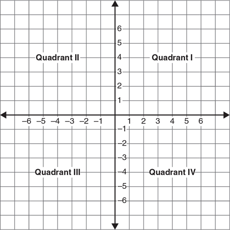
Figure 4.1 The coordinate plane divided into four quadrants.
The x- and y-axes divide the plane into four quadrants. The first quadrant is the section in which both the x- and y-coordinates are positive, and the numbering of the quadrants goes counterclockwise.

Plot each point on the coordinate plane.
1. A(−4, 2)
2. B(8, −3)
3. C(0, 5)
4. D(−2, −6)
5. E(−5, 0)
Tell which quadrant contains the point.
6. (−4, 5)
7. (3, 2)
8. (4, −1)
9. (−2, −2)
10. (3, −4)
Distance
The distance between two points can be calculated by means of the distance formula  The formula is an application of the Pythagorean theorem, in which the difference of the x-coordinates gives the length of one leg of a right triangle, and the difference of the y-coordinates the length of the other. The distance between (x1, y1) and (x2, y2) is the hypotenuse of the right triangle. If the two points fall on a vertical line or on a horizontal line, the distance will simply be the difference in the coordinates that don’t match.
The distance between the points (4, −1) and (0, 2) is


Find the distance between the given points.
1. (4, 5) and (7, −4)
2. (6, 2) and (7, 6)
3. (−7, −1) and (−5, −6)
4. (5, 3) and (8, −2)
5. (−4, 2) and (3, 2)
Given the distance between the two points, find the possible values for the missing coordinate.
6. (a, −2) and (7, 2) are 5 units apart.
7. (−1, 3) and (4, d) are 13 units apart.
8. (8, −6) and (c, −6) are 7 units apart.
9. (2, b) and (2, −1) are 9 units apart.
10. (a, a) and (0, 0) are  units apart.
Midpoints
The midpoint of the segment that connects (x1, y1) and (x2, y2) can be found by averaging the x-coordinates and averaging the y-coordinates.
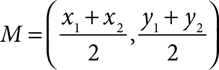
The midpoint of the segment connecting (4, −1) and (0, 2) is


Find the midpoint of the segment with the given end points.
1. (2, 3) and (5, 8)
2. (−3, 1) and (−1, 8)
3. (−5, −3) and (−1, −1)
4. (8, 0) and (0, 8)
5. (0, −2) and (4, −4)
Given the midpoint M of the segment connecting A and B, find the missing coordinate.
6. A(x, 6), B(6, 8), M(4, 7)
7. A(−1, 3), B(x, 9), M(3, 6)
8. A(−5, y), B(7, −3), M(1, 3)
9. A(4, −9), B(−2, y), M(1, −7)
10. A(0, 4), B(x, 0), M(8, 2)
Slope and rate of change
The slope of a line is a measurement of the rate at which it rises or falls. A rising line has a positive slope whereas a falling line has a negative slope as shown in Figure 4.2. The larger the absolute value of the slope, the steeper the line. A horizontal line has a slope of 0, and a vertical line has an undefined slope.
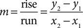
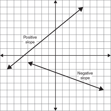
Figure 4.2 Lines with positive and negative slopes.
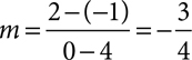
The slope of the line through the points (4, −1) and (0, 2) is

Find the slope of the line that passes through the two points given.
1. (−5, 5) and (5, −1)
2. (6, −4) and (9, −6)
3. (3, 4) and (8, 4)
4. (4, 6) and (8, 7)
5. (7, 2) and (7, 5)
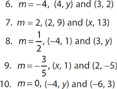
If a line has the given slope and passes through the given points, find the missing coordinate.
Graphing linear equations
A linear equation in two variables has infinitely many solutions, each of which is an ordered pair (x, y). The graph of the linear equation is a picture of all the possible solutions.
Table of values
The most straightforward way to graph an equation is to choose several values for x, substitute each value into the equation, and calculate the corresponding values for y. This information can be organized into a table of values. Geometry tells us that two points determine a line, but when building a table of values, it is wise to include several more so that any errors in arithmetic will stand out as deviations from the pattern.
When you build a table of values, make a habit of choosing both positive and negative values for x. Of course, you can chose x = 0, too. Usually, you’ll want to keep the x-values near 0 so that the numbers you’re working with don’t get too large. If they do, you’ll need to extend your axes, or relabel your scales by 2s or 5s or whatever multiple is convenient. If the coefficient of x is a fraction, choose x-values that are divisible by the denominator of the fraction. This will minimize the number of fractional coordinates, which are hard to estimate.

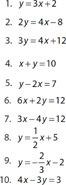
Construct a table of values and graph each equation.
Slope and y-intercept
To draw the graph of a linear equation quickly, put the equation in slope-intercept, or y = mx + b, form. The value of b is the y-intercept of the line, and the value of m is the slope of the line. Begin by plotting the y-intercept; then count the rise and run and plot another point. Repeat a few times and connect the points to form a line.
Intercept-intercept
If the linear equation is in standard, or ax + by = c, form, it is very easy to find the x- and y-intercepts of the line. The x-intercept is the point at which y equals 0, and the y-intercept is the point at which x equals 0. Substituting 0 for y reduces the equation to ax = c, and dividing by a gives the x-intercept. In the same way, substituting 0 for x gives by = c, and the y-intercept can be found by dividing by b. Plotting the x- and y-intercepts and connecting them will produce a quick graph.

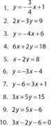
Use quick graphing techniques to draw the graph of each of the following equations.
Vertical and horizontal lines
Horizontal lines fit the y = mx + b pattern, but since they have a slope of 0, they become y = b. Whatever value you choose for x, the y-coordinate will be b.
Vertical lines have undefined slopes, so they cannot fit the y = mx + b pattern, but since every point on a vertical line has the same x-coordinate, they can be represented by an equation of the form x = c, where c is a constant. The value of c is the x-intercept of the line.

Identify each line as horizontal, vertical, or oblique.

Graph each equation.

Graphing linear inequalities
Linear inequalities can also be graphed on the coordinate plane. Begin by graphing the line that would result if the inequality sign were replaced with an equal sign. If the inequality is ≥ or ≤, use a solid line. For > or <, use a dotted line. Test a point on one side of the line in the inequality; the origin is often a convenient choice. If the result is true, shade that side of the line; if not, shade the other side (see Figure 4.3).

Figure 4.3 Graph of a linear inequality in two variables.

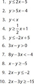
Graph each inequality and indicate the solution set by shading.
Graphing absolute value equations
Many equations involving absolute value have graphs that are composed of two linear segments that have opposite slopes. The graph of y = |x|, for example, is made up of the graph of y = -x when x < 0 and the graph of y = x when x ≥ 0. The result is a V-shaped graph as shown in Figure 4.4.
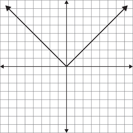
Figure 4.4 Graph of the absolute value equation.
When you start to build a table of values to graph an absolute value equation, first find the value of x that will make the expression in the absolute value signs equal 0. Choose a few values below it and a few above it to fill out your table.
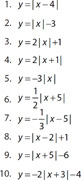
Construct a table of values and graph the equation.
Writing linear equations
It is sometimes necessary to determine the equation that describes a graph either by looking at the graph itself or by using information about the graph.
Slope and y-intercept
If the slope and y-intercept of the line are known or can be read from the graph, the equation can be determined easily by using the y = mx + b form. Replace m with the slope and b with the y-intercept.
Point and slope
If the slope is known and a point on the line other than the y-intercept is known, the equation can be found by using point-slope form: y – y1 = m(x – x1). Replace m with the slope, and replace x1 and y1 with the coordinates of the known point. Distribute and simplify to put the equation in y = mx + b form.
Two points
If two points on the line are known, the slope can be calculated using the slope formula. Once the slope is found, you can use the point-slope form and fill in the slope and either one of the two points.

Write the equation of the line described.
1. Slope = 3 and y-intercept (0, 8)
2. Slope = −5 and y-intercept (0, 2)
3. Slope =  and y-intercept (0, 6)
4. Slope = 4 and passing through the point (3, 7)
5. Slope =  and passing through the point (4, 3)
6. Slope =  and passing through the point (−4, −1)
7. Passing through the points (0, 3) and (2, 7)
8. Passing through the points (3, 4) and (9, 8)
9. Passing through the points (0, −3) and (3, 1)
10. Passing through the points (2, 3) and (8, −6)
Parallel and perpendicular lines
Parallel lines have the same slope. Perpendicular lines have slopes that multiply to −1, that is, slopes that are negative reciprocals. To find the equation of a line parallel to or perpendicular to a given line, first determine the slope of the given line. Be sure the equation is in slope-intercept form before trying to determine the slope. Use the same slope for a parallel line or the negative reciprocal for a perpendicular line, along with the given point, in point-slope form.
To find a line parallel to y = 3x – 7 that passes through the point (4, −1), use the slope of 3 from y = 3x – 7 and the point (4, −1) in point-slope form and simplify.
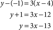
To find a line perpendicular to y = 3x – 7 that passes through the point (4, −1), use a slope of 

Determine whether the lines are parallel, perpendicular, or neither.

Find the equation of the line described.
6. Parallel to y = 5x − 3 and passing through the point (3, −1)
7. Perpendicular to 6y − 8x = 15 and passing through the point (−4, 5)
8. Parallel to 4x + 3y = 21 and passing through the point (1, 1)
9. Perpendicular to y = 4x − 3 and passing through the point (4, 13)
10. Parallel to 2y = 4x + 16 and passing through the point (8, 0)
Calculator notes #3
The primary task of the graphing calculator, of course, is to graph. You practice this with equations that are actually very simple to graph by hand so that you’ll have the skills to produce graphs of more complicated equations. The basics are simple. Press  , clear any old equations, type in your equation, press
  . Of course, there can be other things to think about.
Your equation must be in “y=” form. If you’re trying to graph 3x − 5y = −41, it’s your job to first isolate y.

You don’t have to simplify any more than that, and although it probably runs counter to your training in good practice, it might be better not to do any more. As the equation stands now, you can enter it as Y1 = (−3x − 41)/−5. If you simplify, you’ll have more fractions, and the possibility of sign errors. Notice that the entire numerator is enclosed in parentheses; don’t skip them, because Y1 = −3x − 41/−5 only divides −41 by −5 and produces a dramatically different graph.

When you’ve typed in your equation, you can hit , but you might want to press  and choose 6:ZStandard instead. That sets your viewing window to −10 to 10 on the x-axis and −10 to 10 on the y-axis. Hitting displays whatever window you used last. That might be fine, but it might not. The window is just a portion of the infinite coordinate plane. If you graph the line y = x but your window is set to look at the portion of the plane for which x is between −300 and −200 and y is between 500 and 600, you’re not going to see the line.
If you don’t see the graph, or don’t see enough of it, first press  and notice the coordinates that display at the bottom of the screen. Those are the coordinates of a point on the line. You need to reset the window so that you can see that point. Also think about the y-intercept. Choose the window that seems right to you. Press
  , set Xmin, Xmax, Ymin, and Ymax. You only need to adjust Xscl and Yscl if you’re going to look at a very large window. Set Xscl or Yscl to larger numbers to prevent the tick marks on the axes from blurring together.
Most graphing calculators are not able to graph a vertical line, but may be able to draw one. Press 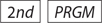 to get the DRAW menu, choose 4: Vertical, and enter the x-value. You cannot trace along this line or find its x-intercept because it is not a graph.