Oz du Soleil is an Excel MVP who’s been working with Excel since 2001. He’s co-author, along with Bill Jelen, of Guerrilla Data Analysis, 2nd edition. Oz has several Excel courses on the LinkedIn Learning platform. He’s best known for the dramatic and colorful Excel tutorials on his YouTube channel Excel on Fire.

Data cleansing is Oz’s area of specialization in Excel. From his earliest days with Excel, he has found himself constantly needing to fix names that are ALLCAPS, peel addresses away from phone numbers, clean up the messes that result from extracting data from PDF files, and fix all the many other things that prevent data from being useful.
Oz has presented Excel topics and master classes at conferences in Amsterdam; Sofia, Bulgaria; São Paulo, Brazil; Toronto, Canada; and cities around the United States.
When Oz isn’t elbows-deep in the guts of a spreadsheet, he does storytelling around Portland, Oregon. He has told stories onstage for Risk!, Pants on Fire, Seven Deadly Sins, Pickathon, The Moth, and other storytelling shows.
Thanks to MrExcel, Bill Jelen, for the opportunity to share one of my favorite Excel topics.
A newspaper reporter once described to me the problem she had in getting the public school system to turn over data that it was legally required to turn over. In the face of school closings and outraged parents, the mayor and school administrators kept repeating things like “the data say…” and “the data tell us…”—and the reporter wanted to see this omniscient data.
She eventually did get the data, and it was a mess. The law didn’t require the data to be free of duplicates and ready to be sorted, filtered, and analyzed. And that’s where the investigation ended because the reporter didn’t have the skill or resources to cleanse the data.
Lawyers have complained about similar problems. The opposing side is required to provide data—but that data doesn’t have to be immediately useful. Someone has to take emails, PDFs, and reports from various banks, PayPal, QuickBooks, etc.; get the formats all the same; and then merge them together before any analysis can happen.
Without clean data, no analysis can happen.
This Straight to the Point guide provides an introduction to data cleansing, which also goes by names such as data munging and data wrangling. Whatever the name, it basically means doing what needs to be done to make data useful and trustworthy. Data cleansing can include the following tasks:
- Deleting unnecessary headers
- Deleting summary rows
- Filling in gaps
- Flattening a report
- Merging and appending data from multiple sources
- Pulling data from source X to complete data in source Y
- Splitting names from addresses
- Identifying and deleting duplicate records
- Converting units of measurement in multiple sources
- Transposing data so it appears in columns rather than rows
A program coordinator is all set to analyze some survey results and—oh, no!—the information looks like this:
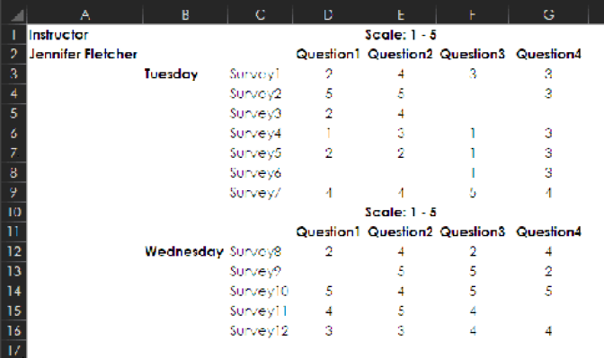
The program coordinator would like to do a lot of things with this data, including the following:
- Make graphs
- Sort it
- Get summaries about all 12 surveys
- Get a summary for each day to see if one day fared better than the others
- Extract all responses that are 1 or 2 and see if there’s anything interesting
But in its current format, this data can’t be used in any of these ways. It would be possible to write delicate complex formulas to analyze the data in its current shape, but not a lot of people have the skills to do that. In any case, there’s a much more powerful way to make this data usable: Cleanse it by turning it into a “flat file” of plain rows and columns, without extra headers and titles. (You’ll learn more about flattening a report in the section "FROM USELESS TO USEFUL: FLATTENING A REPORT" on page 47) Once you’ve turned this report into a flat file, the world is wide open: You can generate a variety of reports, easily merge this data with other flattened data, share it with someone who needs this source data for purposes different from yours, upload it to a database,…ANYTHING!
The sad fact is that many people who are taught to analyze data are not taught about data cleansing, and many people—like the reporter mentioned earlier—are stumped when they encounter messy data. A marketing student is likely to be taught analysis on clean data. When he gets out of school, if he’s handed data that’s locked in a PDF and that turns into an atrocious mess when it’s extracted from the PDF, will he know what to do with it? Probably not. If he learns data cleansing as a skill, however, he won’t panic when he encounters such data messes. He will be able to develop a confident strategy for extracting data gold from the mud, rocks, and even permafrost.
The Straight to the Point Ethos
Data cleansing is the topic of this short book, and I’m excited to share it with you because this book doesn’t focus on a specific Excel feature. Instead, it is about strategy and getting things done with whatever is available in all of Excel. This book digs into some of the most common data cleansing needs and focuses on strategy and context. (Sometimes, for example, a down-and-dirty one-time solution is most efficient, and other times a Power Query solution that’s more suited for repeated tasks is the best approach.) In the section "COMPARING LISTS: WHAT’S OVER HERE THAT’S NOT OVER THERE?" on page 7 you’ll see multiple solutions for the same problem, followed by a summary of how to pick the best strategy for claiming victory over uncooperative data in a particular set of circumstances.
Say that you’ve got a list of names that are messy—a mix of ALLCAPS, all lowercase, and Proper Mixed Case. Maybe you need to print mailing labels and realize that the names are not going to work if you leave them as they are.
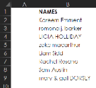
One way to fix them is to use Excel’s Flash Fill. To start, you have to train Flash Fill on what the desired results should look like. In the example below, you would start by typing Kareem Emment in C2. Then, as shown below, when you type the R for Romona, Flash Fill presents the ghosted (or grayed) text as a preview, as if to ask “Is this what you want?”

If you were to press Enter at this point, the entire ghosted list of data would be committed as actual text. However, that ghosted result isn’t what you want here because most of the names aren’t correct. This is a good example of how you have to keep training Flash Fill by giving it more examples of the desired result.
As shown in the next image, you can keep training Flash Fill by typing the corrections Romona J. Barker and Mary & Gail Dorsey.
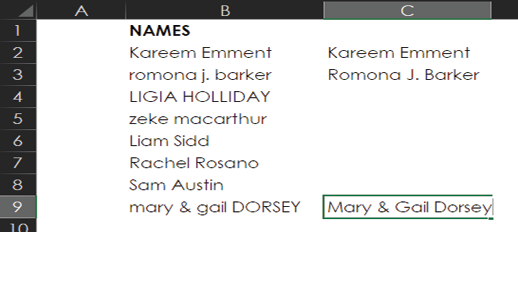
This should give Flash Fill enough information to know that you want to capitalize the first letter of each name. So next you can select Data > Data Tools > Flash Fill, as shown below.
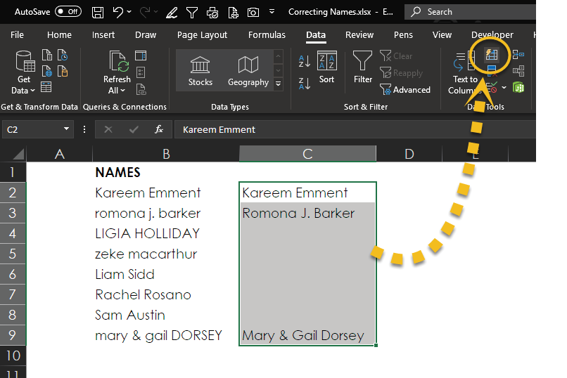
As you can see, the result is beautiful!


Oh, well, the result is almost beautiful. In row 5, Zeke MacArthur’s name should include a capital A. This is one of those situations where Excel can get you 99.999% of the way to where you want to be, but you need to understand both your data and Excel to know where there could be trouble spots.
Here you can see what Flash Fill does with some tricky names.

So, after using Flash Fill, you need to go back, check your results, and manually make any corrections to issues such as these. If you’ve got a list of 500 names and need to manually correct 3 of them, Flash Fill has been a huge help!
NOTE: The results of Flash Fill are final. They are not dynamic, and they involve no formulas. Thus, Flash Fill is good for one-time or infrequent needs. For a dynamic solution, you should instead use formulas or Power Query.
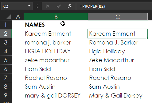
In the olden days, fixing the case of names would have required the PROPER function. You can still use this function today, and it is what you could use if you needed a dynamic fix rather than Flash Fill’s one-time static fix. Be warned, though: PROPER runs into the same problem with turning MacArthur into Macarthur, so you still have to check the results to see if any adjustments are needed.
COMPARING LISTS: WHAT’S OVER HERE THAT’S NOT OVER THERE?
It’s difficult to avoid working with lists. People who do all sorts of things with data and who have all kinds of different roles have to deal with comparing, merging, or segmenting datasets. These are some of the reasons you might need to compare lists:
- One list indicates what maintenance needs to be done, and another list indicates what maintenance has been done.
- One list shows what’s supposed to be in inventory, and another list shows what is actually in inventory.
- List A indicates who paid for a trip, and List B tells who went on the trip.
How do you compare lists like these to uncover similarities and differences? Keep reading, and you’ll learn the secrets!
Invitations and Responses (Match It All Up!)
This example shows one list of people who were invited to an event and a separate list of people who have responded. In addition, there is data that you’d like to match up for the people in the two lists. For example, you’d like to be able to easily see that Dacia Cohen was invited and plans to bring two guests, and you want to get her email address alongside her name in case you need to contact her.
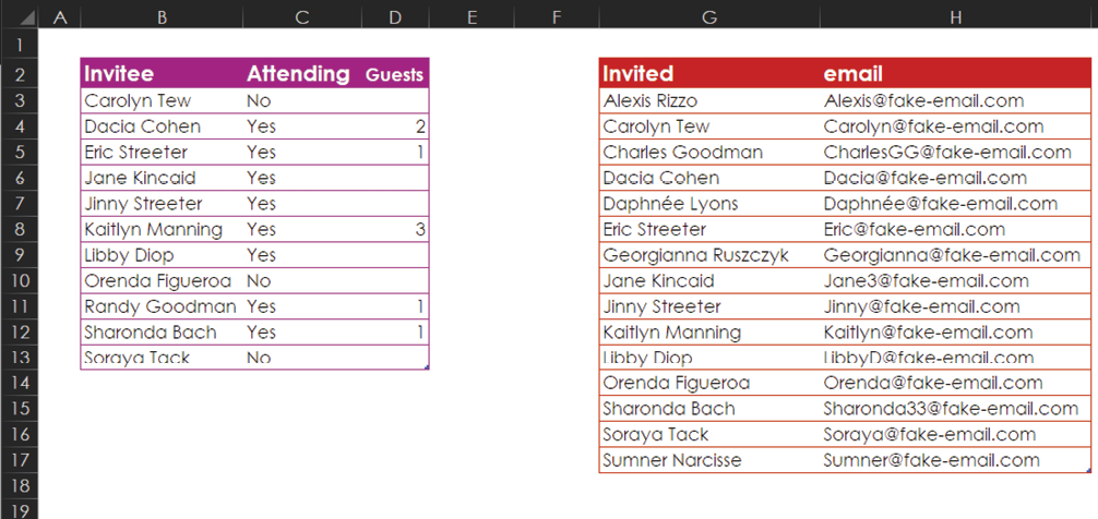
To do everything you want to do here, the best strategy would be to create a master dataset via a Power Query Full Outer Join. This is the best strategy for two reasons:
- The Full Outer Join will match everything that has a match.
- Power Query can be easily updated when you modify the data.
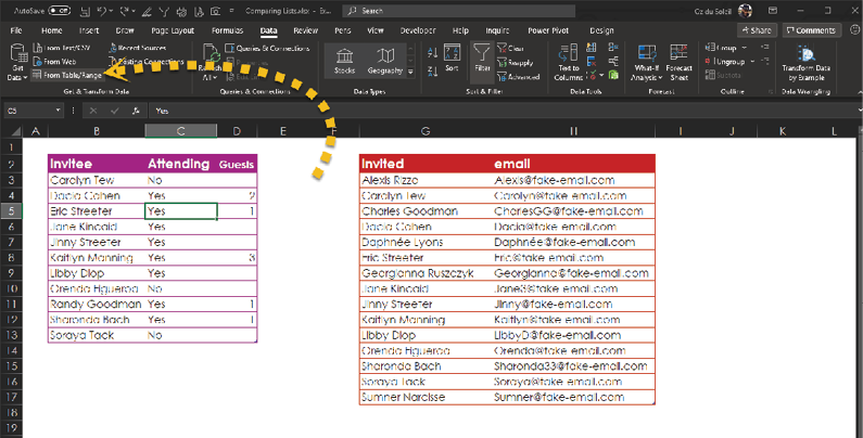
The datasets are already in tables, so you need to make queries. With the cursor in the Invitee dataset, select Data > Get & Transform Data > From Table/Range, as shown below.
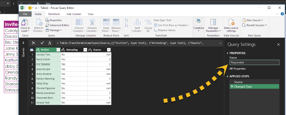
Excel takes you to the Power Query Editor, where you are going to do only one thing: Change the name of the query to Responded, as shown with the arrow below.
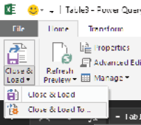
Then, in the upper-left corner, click the arrow underneath Close & Load and select Close & Load To.
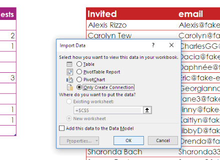
Excel opens the Import Data dialog box, which you can use to tell Excel where to load the result. In this case, you should select Only Create Connection because this is an intermediate step with results that you don’t need on a worksheet; you just need the query so that you can merge it with the next query.
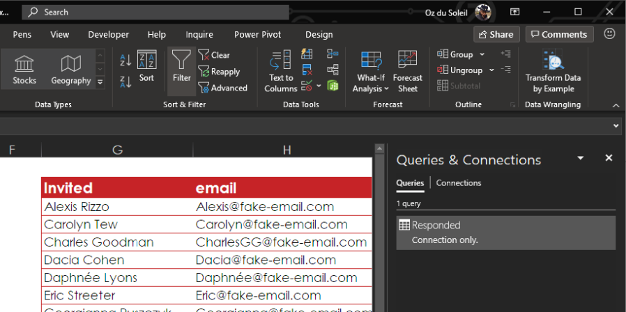
Now, in the Queries & Connections pane, you see the Responded query.
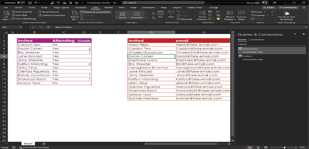
Now you need to follow the same steps again, this time starting in the Invited table. Name this query Invited and load it as a connection only.
When you have the two queries, as shown below, you’re ready to merge them and get everything matched up.
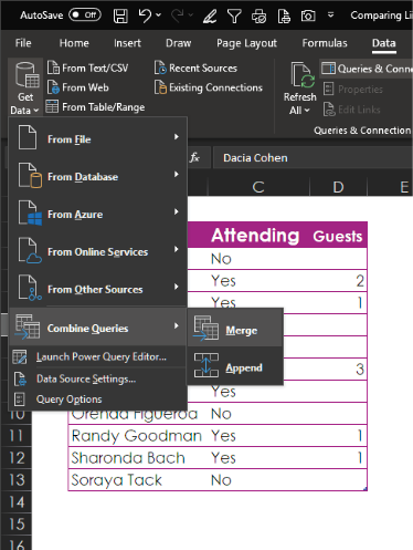
To start the merge, select Data > Get & Transform Data > Combine Queries > Merge.
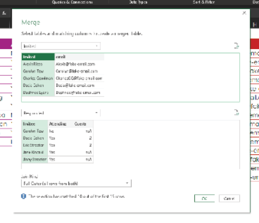
In the Merge dialog box, you see the Invited query at the top and the Responded query at the bottom. Highlight the columns that need to be matched—in this case, Invitee and Invited. For Join Kind, at the bottom of the dialog, select Full Outer. Then click OK.
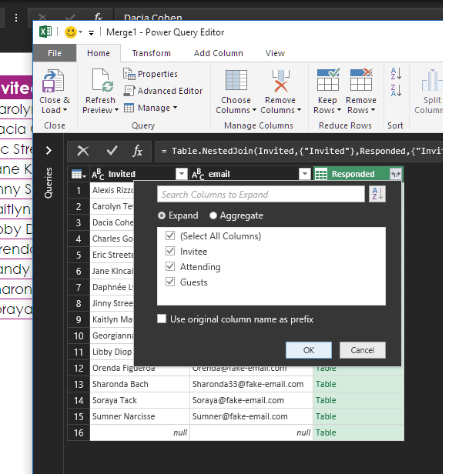
In the Power Query Editor, you can see the Invited query, and the Responded query’s data is collapsed in the Responded column. Click the double arrow at the top of the column and deselect Use Original Column Name as Prefix (because all it does is make a big ugly column header that you don’t need; try it out if you want).
Click OK, and you see all the data, now matched up wonderfully.
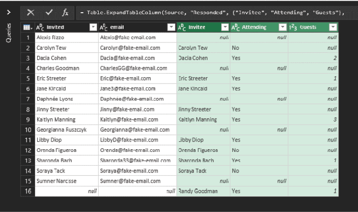
Here are some of the things you can see in the data:
- You haven’t heard from Alexis Rizzo yet.
- Dacia Cohen is attending and bringing two guests.
- There are 16 unique people.
- Soraya Tack is not attending.

Wait a minute. What’s the deal with Randy Goodman? She wasn’t invited, but she’s showing up as not only attending but as bringing one guest. Who is Randy Goodman?
NOTE: Randy Goodman shows why you did the Full Outer Join here rather than a simple MATCH or VLOOKUP. If you had only asked “Who haven’t we heard from?” you would not have discovered that you heard from someone who wasn’t even invited. Therefore, when comparing lists like this, it’s critical to not only compare List A against List B but also compare List B against List A.
For the time being, you can simply click Close & Load, and you see the final dataset along with a new query named Merge1, as shown below.

Now send someone to find out who Randy Goodman is!
Determining What’s over There That’s Not over Here
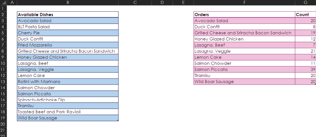
A common data analysis need is to determine what’s in one list that isn’t in another. There are a few ways to find this information: by using a formula, by using dynamic arrays, or by using a Power Query Anti Join. The following sections show how to use all three methods, using the example of a catering company that wants to find out which of its available dishes have never been ordered. Each of these methods has pros and cons, and they’re all especially useful in different scenarios.
Available vs. Ordered: Formula Method
As you can see above, both datasets—the available dishes and the ordered dishes—are in tables. To find out which of the available dishes have never been ordered by using a formula, you can start a new column named Match in cell C2. In cell C3 you then use this formula:
=MATCH([@[Available Dishes]],Table1[Orders],0)
Every entry with #N/A means that the available dish was not found in the list of orders. A number in the Match column indicates the position in the orders list where the dish was found; for example, lemon cake was found seventh in the list of orders.

This is a down-and-dirty one-and-done method: You write one formula, and you get an answer. This is the strategy to use if you just need an answer now and don’t expect to ever need to know such information again.
But what if learning which dishes aren’t ordered becomes a regular need? If you keep using the formula you’ve just created and new orders and new available dishes are regularly added to the tables, the #N/A errors will sooner or later become unbearable visual clutter. In such a case, you might instead choose to use dynamic arrays or Power Query to create a summary of just the items that have never been ordered. The following sections describe these two methods.
Available vs. Ordered: Dynamic Arrays Method
Dynamic array functions and the new Excel calculation engine were released to Office 365 Insiders in September 2018—and they’re spectacular!
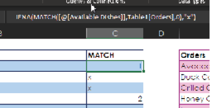
To see how dynamic arrays work, you can look again at the previous example but now wrap the MATCH function in IFNA, as shown here:
=IFNA(MATCH([@[Available Dishes]],Table1[Orders],0),”x”)
In column H you create a NEVER ORDERED section. Then, in cell H3, you use the new FILTER function, like this:
=FILTER(Table2,Table2[MATCH]=”x”)
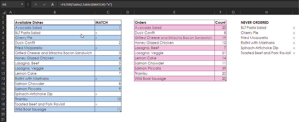
The NEVER ORDERED column now lists all the dishes that have never been ordered. It’s so easy!
But wait.…There’s more! Scroll down and unhide rows 30 through 36, and you see that there are more items in both the available and orders lists, as shown below.

Now add the data from rows 30 through 36 to the data above by dragging it up to the respective tables.
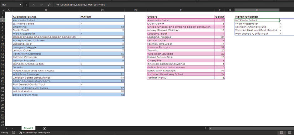
Holy moly! The dynamic array—that is, the NEVER ORDERED list—has updated. You wrote just one formula and didn’t have to refresh anything, as you’d have to do with a PivotTable or Power Query.
Available vs. Ordered: Power Query Anti Join Method
Now it’s time to see how Power Query can help you create a summary of just the items that have never been ordered. This method involves a Power Query option known as an Anti Join. A Left Anti Join can be thought of this way: Give me everything that’s on the left side that does not have a match on the right side.
In the Venn diagram below, say that you’re looking at two sets of people: those who live in Chicago and those who work in Chicago. You can see that there’s some overlap, and a number of people, like Leo and Trudy, fit both criteria (that is, they both live and work in Chicago).
A Power Query Left Anti Join isolates the people who live in Chicago and do not work in Chicago—the boldface list on the left below.

To apply a Left Anti Join to the available vs. orders example, you should create an Available query and an Orders query, as shown below.

You can merge the Available and Orders queries to create a Never Ordered dataset. To do so, select Data > Get & Transform > Get Data > Combine Queries > Merge.
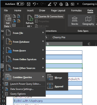
Power Query brings you to the Merge dialog box, where you select the Available query at the top and the Orders query at the bottom.
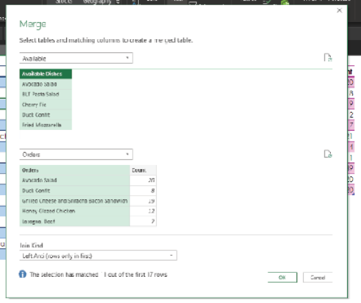
To let Power Query know what you want to match, highlight the Available Orders and Orders columns, as shown below. For Join Kind, at the bottom of the dialog, select Left Anti. Then click OK.
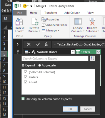
Inside the Power Query Editor, the left-side data (the Available query) is visible. The right-side data (the Orders query) is collapsed in the Orders column.

Click the button with the diverging arrows and, in the dialog that appears, deselect Use Original Column Name as Prefix.
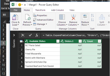
Woah! You get nothing but nulls in the Orders and Count columns. Why? The Left Anti Join retrieved everything on the left side that does not have a match on the right side—exactly what you were looking for.
Highlight the Available Dishes column, right-click, and select Remove Other Columns.
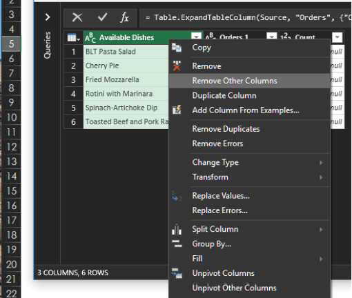
Now click Close & Load.
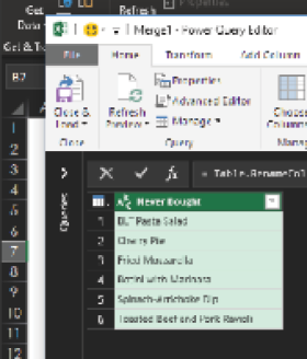
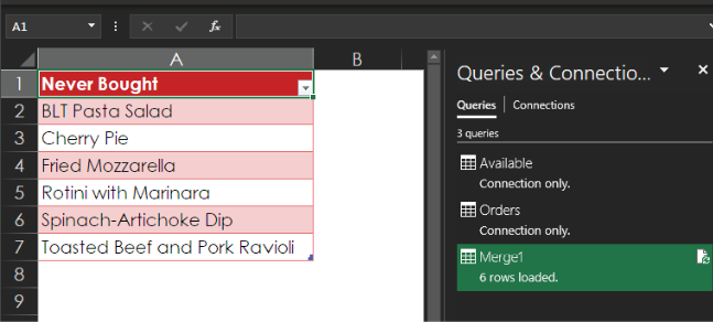
And here is the result:
On the sheet with the original data, scroll down and unhide the additional data in rows 30 through 36.
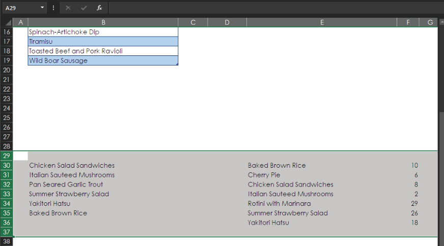
Now add the data from rows 30 through 36 to the existing data, as shown below.
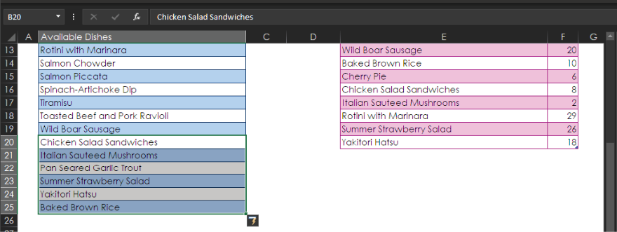
To apply the query steps to the new data, select Data > Queries & Connections > Refresh All. Bang! You get a new result, as shown below.
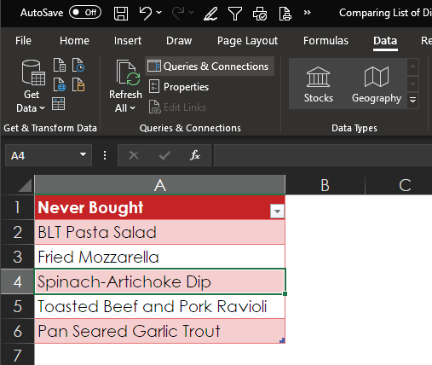
You’ve just seen three ways to find the same information using various Excel tools. Which one is best? The answer depends on your context. You have to understand your complete need and determine what you are comfortable with. Let’s review:

PEELING, PARSING, AND SEGMENTING
This section looks at the classic problems involved in separating bits of data that are stuck together—a task sometimes referred to as parsing strings of text.
Extracting the First Name (Using Flash Fill)
Parsing strings of text can be a nightmare. For example, say that you have people’s names and cities all in one column, as shown below.
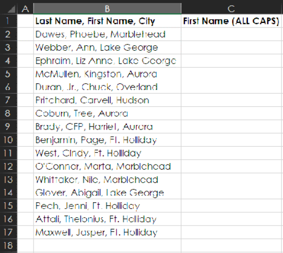
Now suppose you’re having an event and would like to print nametags that have each person’s first name in ALL CAPS. To make that happen, you have to parse the data to get those first names out of the first column.
The details in the first column are separated by commas. Note, though, that rows 6 and 9 have additional commas, which complicates the situation. If you tried to use Excel’s Text-to-Column feature here, it would create a mess for you—and more work—because it would separate the data at every comma and put Jr. and CFP into a column with the first names. This is the first of two reasons you don’t want to use Text-to-Column here.
The second reason you don’t want to use Text-to-Columns in this case is that Flash Fill can help you do the job much more easily. However, with Flash Fill, you have to think ahead. Because of the extra commas in rows 6 and 9, you have to do some extra training to help Flash Fill recognize the pattern.
You can start by typing in PHOEBE in C2. Then, as soon as you type A in C3, Flash Fill’s ghosting lets you know that it will give you the wrong results for rows 6 and 9.

To properly train Flash Fill, you can press Esc and type in CHUCK and HARRIET, as shown below.

Next, highlight the entire column where you want the final names to appear and choose Data > Data Tools > Flash Fill.
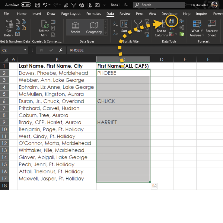
As you can see below, this does the trick, and you get exactly what you wanted!
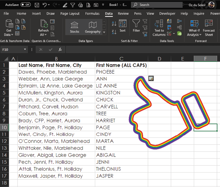
Splitting by a Single Delimiter: Separating the City from the Name
Now, using the same data as for the nametag example, say that you need to separate the names from the cities. This would be easy enough to do with Flash Fill, but what if you’ll be adding more data to the list and need to repeat the parsing of the names from the cities? Two words: Power Query!

With the cursor in the dataset, you start a Power Query solution by selecting Data > Get & Transform Data > From Table/Range. As shown below, select the checkbox My Table Has Headers. (Yes, the table does have headers.)
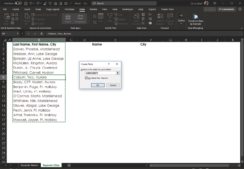
With the column highlighted, select Home > Split Column > By Delimiter.

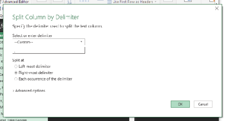
Next, you need to configure the Split Column by Delimiter dialog settings as shown in the image below. One thing that’s vital that you cannot see in the image below is that the custom delimiter is a comma with a space after it. That is, you need to split by a comma and a space, not just a comma. If you do this, you won’t end up with leading and trailing spaces when you’re done with the splitting, and you won’t have to take the extra step of clearing those extra spaces. There’s no reason to work that hard today.
Also note in the image below that you need to split at the right-most delimiter. The Right-Most Delimiter option is beautiful because it allows you to surgically parse strings of text rather than use the ham-fisted Text-to-Columns feature.
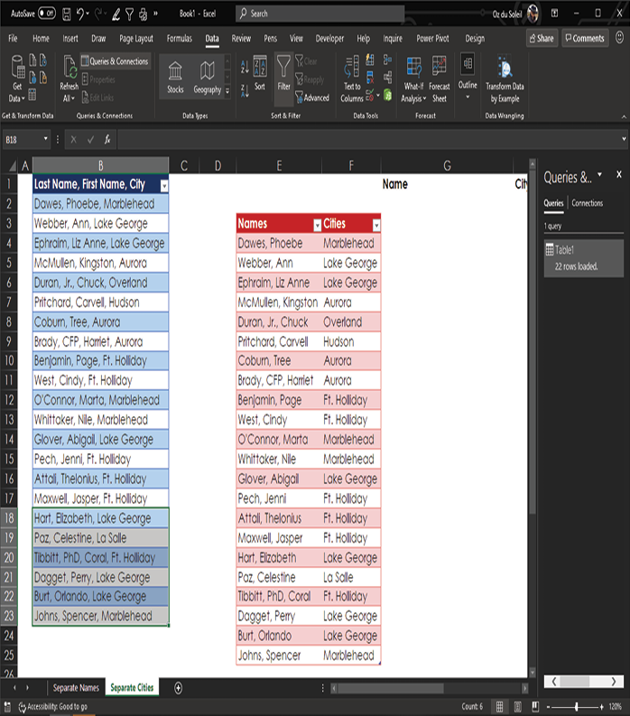
Click OK, and you see the result below. Done! Split! You got it!
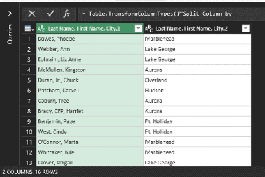
The last step is to rename the columns Names and Cities. Double-click the column heading and type a new heading.
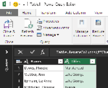
Next, select Close & Load > Close & Load To and load the query result to start in cell E3, as shown below.
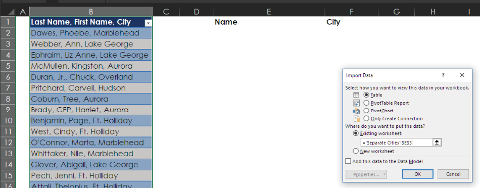
The result, as you can see here, is a beautifully cleansed dataset with names formatted consistently and correctly in one column and cities in another column.

As hinted at earlier, the benefit of doing this in Power Query is that if you add more data, Power Query applies the same data cleansing to the new data for you. To see how it works, go back to the source data, scroll down, and unhide the data in rows 25 through 30.
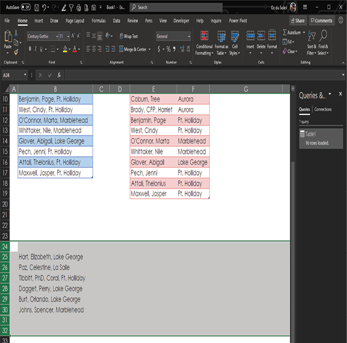
Drag that data into the table of names and cities above.
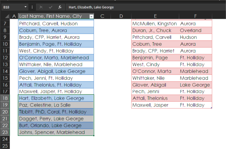
Now all you have to do is refresh, and Excel reruns the query with the new data. Select Data > Queries & Connections > Refresh All, and there’s the newly added data, looking just the way you want it!
Splitting into Rows: Getting Those People Out of There!
Now let’s look at the classic problem of too much stuff in a single cell. This often happens when data is copied from an email or a web page and then pasted into Excel. To see how to deal with this issue, say that you have guests and their table assignments, as shown below.
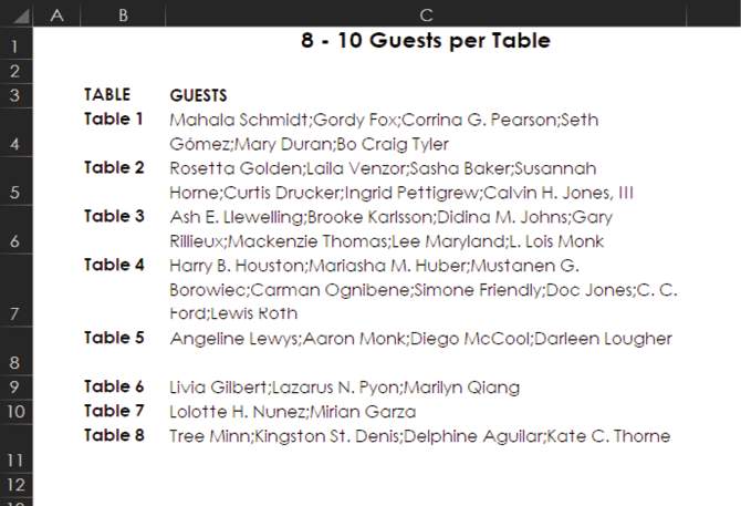
Because of the way the data is formatted, you can’t do any of the following operations:
- Sort by name
- Easily count how many people are at each table
- Identify any duplicate names
How can you cleanse this data so that it’s useful? Use Power Query!
Place the cursor in the data range and select Data > Get & Transform Data > From Table/Range.
In this case, you can take advantage of the fact that the names are separated by semicolons. Inside the Power Query Editor, highlight the GUESTS column and then select Home > Split Column > By Delimiter.
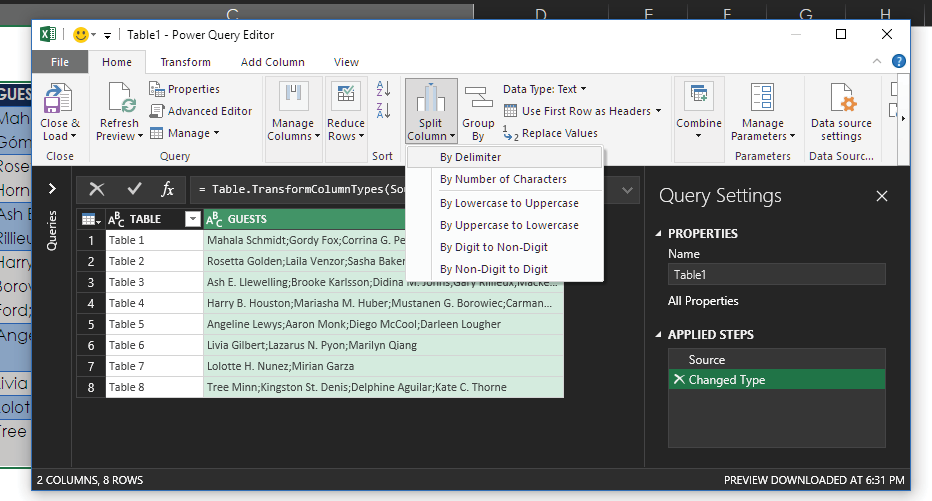
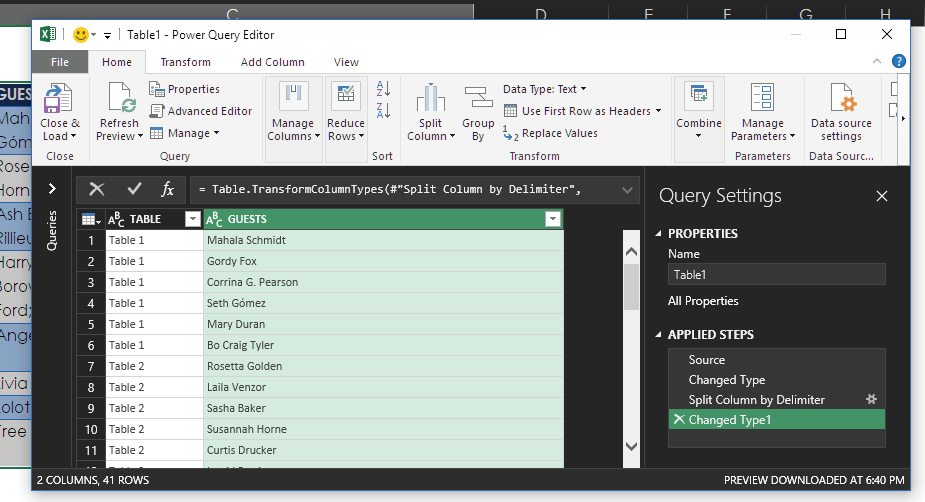
As shown in the image below, you can indicate the semicolon as the custom delimiter and select Each Occurrence of the Delimiter to split at each semicolon. Then expand the Advanced Options section and choose Split into Rows. Finally, click OK.
And here you can see the final data—ready for use!
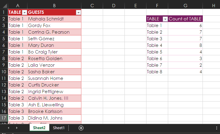
Click Close & Load, and you see the table shown at left below. You can also create a PivotTable, as shown at right below, to tally the number of people at each table.
IDENTIFYING DUPLICATE RECORDS: FUZZY MATCHING
Duplicate records are insidious. They create problems ranging from mildly embarrassing to catastrophic.
These are some of the many ways duplicates can end up in a dataset:
- Customers go online and create multiple accounts for themselves—deliberately or accidentally.
- Someone compiles data from multiple data sources, and it turns out that some entries exist in more than one of the sources.
- Sloppy copy/paste jobs happen all the time.
Duplicates in data can cause simple consequences like the embarrassment of mailing two duplicate pieces of mail to the same person. But duplicate records can also cause big problems, like jeopardizing someone’s professional license—which I’ve actually seen happen. That kind of problem causes a great deal of undue stress!
Excel’s Duplicate Remover: The Hazard!
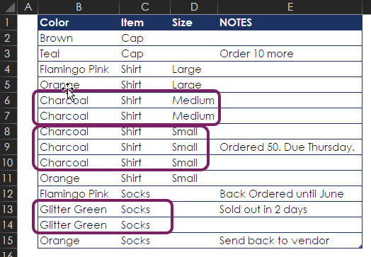
Let’s look at a simple example of identifying duplicate records. Say that you have a list of 14 records, as shown here, and you’d like to know how many unique items you have. You really don’t have 14 items, though: It’s easy to see that small charcoal shirts is entered three times, medium charcoal shirts is in here twice, and glitter green socks is entered twice.
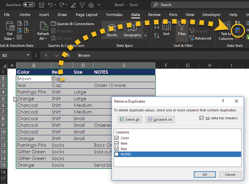
Excel has a duplicate remover that can help out here. Select Data > Data Tools > Remove Duplicates. Then, in the Remove Duplicates dialog box, select all columns except NOTES.

Look at what happens when you click OK. Excel picks the items to get rid of. Its results are fine if you don’t care about the notes and really wanted just a list of the unique items. But if you did need that note about the charcoal shirts that are due Thursday, you’re in trouble because that note is now gone.
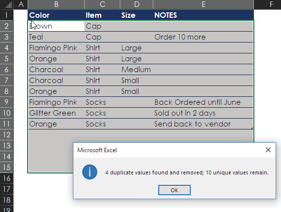
The moral of the story: Use Excel’s duplicate remover only when it’s okay for Excel to pick what to delete. The next section shows a safer way to find duplicates. In that section, you will also get a taste of what’s formally called fuzzy matching.
Reality, Context, and Strategy: Flagging Records for Review Instead of Clearing Duplicates
Fuzzy matching is the sometimes grueling task of matching entries that aren’t identical. It can be as simple as using an employee ID to match Kate Montgomery with Kate A. Montgomery. In more difficult cases, you have to deal with entries that have multiple legitimate variations, like these:
- 18th Avenue Library
- Cora & Lloyd Prudhomme Memorial Library
- 1904 18th Ave
- City Library—Clock Tower Branch
At this level, matching duplicates can be an art, or it can be tedious. You have to decide how much effort to put into this and when it’s time to accept that the data won’t ever be 100% clean.
When you’re looking for duplicates, it’s important to think about context and strategy. In the previous example, you let Excel delete duplicates for you. However, when you’re out in the real wilderness, battling messy data, it’s often better to flag potential duplicates and check a couple issues:
- Are they truly duplicates?
- If they are duplicates, which one(s) should be kept, and which one(s) should be deleted?
To take a peek at how this can play out, consider the data in the following example.
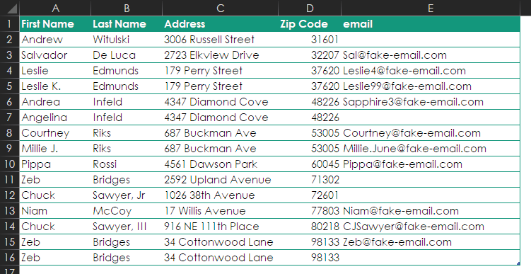
The data here is just foul:
- Leslie Edmunds and Leslie K. Edmunds are the same person.
- Excel’s duplicate remover would not identify these records as duplicates even though they are for the same person.
- Two email addresses are listed for Leslie. Which one should be kept? Does it matter?
- Zeb Bridges is in here three times. (Let’s assume that we know this is the same person.)
- He has two different addresses.
- One record has an email address. Whatever you end up doing with Zeb, you want to keep the email address.
- A decision has to be made about the two addresses. Do you keep both? Keep the one with the email address? Mail a letter to both addresses and ask Zeb for verification? Just get rid of one because the consequences aren’t very high if you get it wrong?
- If you tried to clear duplicate addresses, you would eliminate people who live together, such as Courtney and Millie Riks.
Because of these wrinkles, this is a case where it’s best to flag possible duplicates for review rather than let Excel just delete them for you. You also need a lot more information based on the context. What are the stakes if you get the results wrong? Consider:
- If you’re mailing a $2 coupon for shoelaces, then it’s not a big deal if some people get more than one and you delete some people that you incorrectly identified as duplicates.
- If you’re about to contact them to announce that they’re under investigation for professional impropriety, you’ve got to get this right.
One trick for flagging duplicates is to create a unique identifier, such as the ones in column F below, and then use conditional formatting on it. In this case the ID in column F is built from pieces of the source data, using the following formula:
=LEFT([@[First Name]],4)&[@[Zip Code]]&RIGHT([@[Last Name]],5)&MID([@Address],2,4)

The formula takes the following information:
- The first four characters of the first name
- The whole zip code
- The last five characters of the last name
- Four characters from the address, starting with the second character
Next, to use conditional formatting to flag possible duplicates, highlight the ID column and select Home > Styles > Conditional Formatting > Highlight Cell Rules > Duplicate Values.
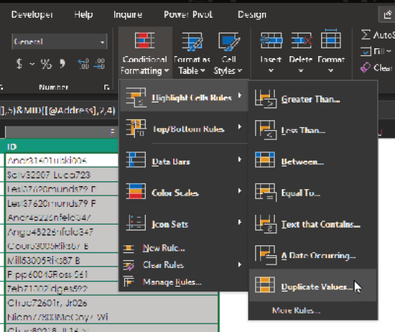
And here is the result:

Both Leslies and two of the three Zebs are flagged. You could delete one of the Leslies and one Zeb, but you know you have a third Zeb. How you approach the situation from here is all about strategy and deciding how much effort is needed to get the data to an acceptable level of cleanliness.
If you need a result that’s better than this, you might work on the list in chunks. For example:
1.Separate all records that are clearly, without a doubt, unique. Get them out of the way.
2.Flag unique addresses. Isolate them and identify duplicates vs. multiple people with the same address.
3.Flag unique names. Isolate them to identify duplicates vs. different people with the same name.
4.Use more than one unique identifier to isolate possible duplicates in different ways.
5.As records get verified as unique, move them over to the first list that you know is clean.
6.At the end, there are usually a few very difficult entries that can only be handled manually—perhaps even by finding contact information and asking the people themselves for corrections.
How far you go depends, again, on the stakes.
MERGING AND APPENDING MULTIPLE WORKBOOKS
Now say that you have a folder named FolderImport, and it has five files containing data that you’d like to have stacked up in one place. In this case, you are ordering shirts for all active members and need to know how many of each size to order.

The files look like this:
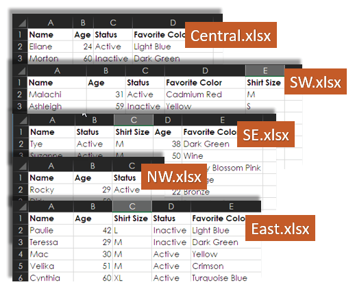
You can quite easily make the following observations about these files:
- All the files start with a Name column, and that’s all that’s similar in all five of the files.
- NW.xlsx just has Name, Age, and Status columns, and it’s the only file that doesn’t have a Favorite Color column.
- East.xlsx, SE.xlsx, and SW.xlsx have the same columns, but they aren’t in the same order.
Before Power Query came along, getting this type of data stacked up was a copy/paste nightmare. It is now much easier to merge these files: Start by opening a new workbook and then select Data > Get & Transform > From File > From Folder.
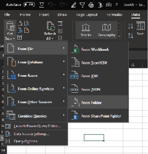
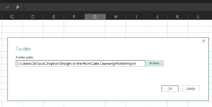
Navigate to the location where you’ve stored the FolderImport folder.
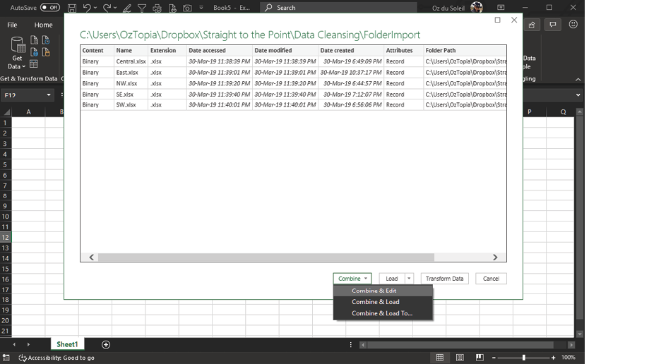
Next, you see a list of all the files in the folder. Select Combine & Edit.
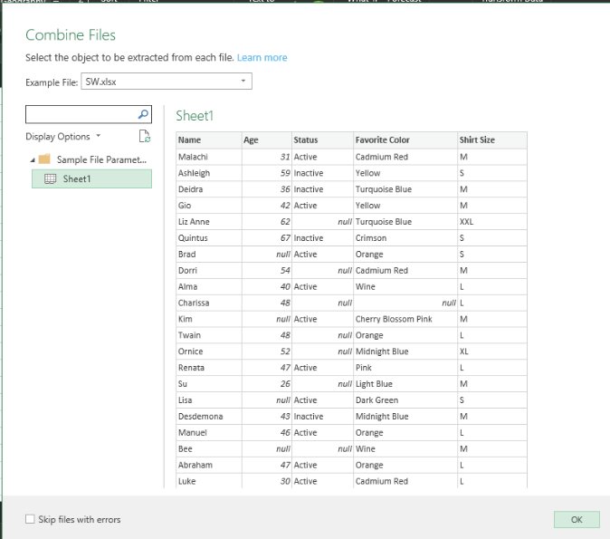
In the Combine Files dialog box, highlight Sheet1. In the Example File drop-down, you have to select one of the files that has all of the headers—so in this case, select SW.xlsx.

If you select NW.xlsx for Example File, Power Query will import only the three columns contained in that file.
Here is the data! Everything from the five files has been merged, and the columns are all lined up. You’re done!
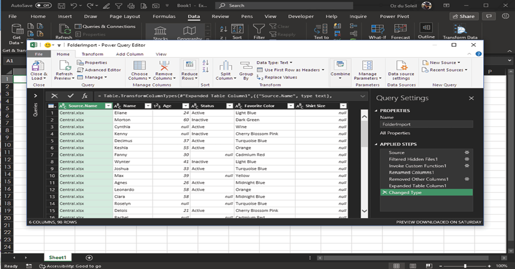
NOTE: Notice that Central.xlsx doesn’t have a Shirt Size column, and Power Query handles this by adding a column, adding the column heading Shirt Size, and filling the column with null.
Now select Close & Load, and the result is 98 rows of data from the five source files.

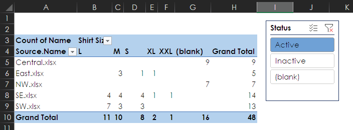
If you add a PivotTable and a slicer and filter for only active members, you see that you need 16 more people to let you know their shirt sizes.
FROM USELESS TO USEFUL: FLATTENING A REPORT
A common and often useless starting point for data is a report format. A report is designed to give human beings a predefined view of specific data to answer specific questions. However, what if the report does not answer the questions you’re asking? In this situation, you need a different view of the data, but it might be difficult to get someone to generate a nice pretty report for you. In such cases, it is incredibly helpful to be able to flatten a report into a flat file—that is, turn the report into a simple wall of rows and columns of data. The flattened result isn’t easy for a human to read. However, flattening a report makes it infinitely easier for a human to get Excel to generate any imaginable report that’s based on the data.
Below, the survey results on the left can tell you that Jennifer Fletcher captured 12 surveys over the two days that she presented, and you could use the information shown to calculate some averages. The survey results on the right have been flattened, and although the data isn’t pretty, it’s now in a format that will allow you to look for many other insights:
- You could put the flattened data into a PivotTable or a data model.
- You could sort by scores, largest to smallest.
- You could insert slicers to toggle between results for Tuesday, Wednesday, and both days.
- You could merge this data with data from other sessions to enable more complex analysis.
The ability to flatten data makes you practically invincible.

In this section, you’re going to use Power Query to flatten the data from the survey report shown above. But you’re not going to use From Table/Range. Putting the report into a table would be a bit goofy because the report has headers all throughout; it has different sections that don’t go together; and in some situations, reports like these have empty columns and rows that you could easily miss if you’re not paying attention.
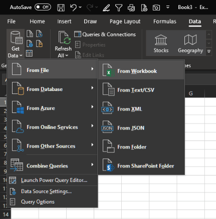
Rather than use a table, it’s better to open a brand-new workbook and import the entire worksheet. So, with a new workbook open, select Data > Get & Transform > Get Data > From File > From Workbook.
You now see the Import Data dialog, in which you need to navigate to the location where you have stored the file Survey Results.xlsx.
NOTE: This technique creates a file path between the new Excel workbook and the source workbook. If you anticipate that changes will be made to the source data, you need to store the source workbook in a location that is not likely to change. If the location does change, you need to get into the query and navigate to the new source location.
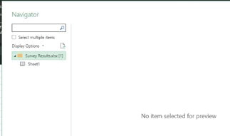
The Navigator pane gives you a preview of the data, and you can choose to import the entire workbook Survey Results.xlsx or just Sheet1.
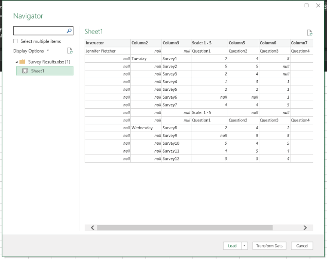
In this case, you want to select the folder to import the entire workbook. Then click Transform Data.
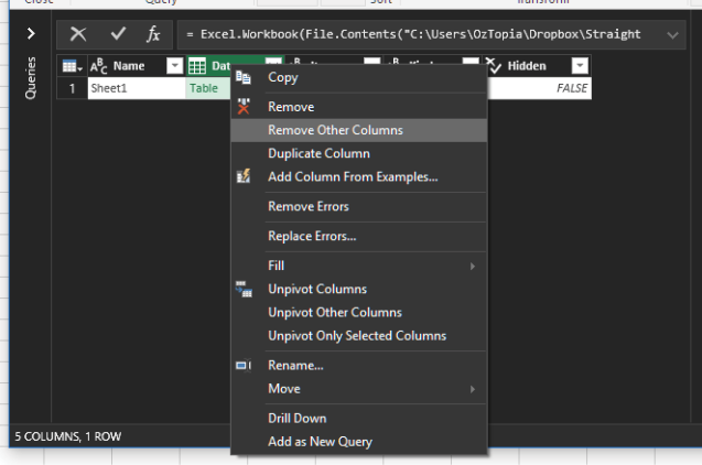
The dataset is in the collapsed Data column, and in this case you don’t need the other columns.

Highlight the Data column, right-click, and select Remove Other Columns.
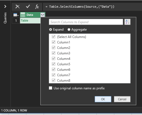
Click the diverging arrows to expand the column and deselect Use Original Column Name as Prefix.
After you click OK, you see your fabulous data, all ready to be flattened.
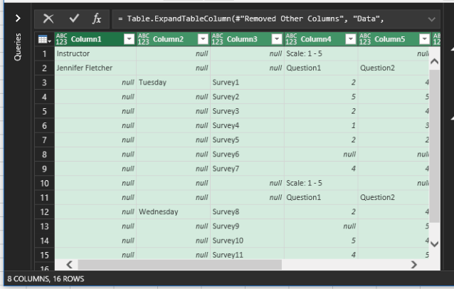
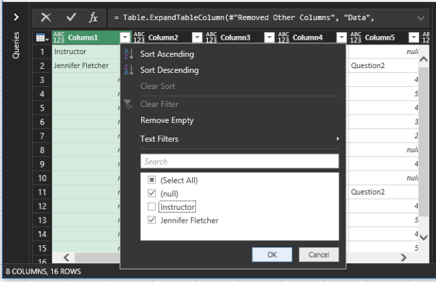
It takes several strategic steps to convert the data from its current format into a wall of columns and rows. First, you don’t need the very top row, so filter Column1 and deselect Instructor.
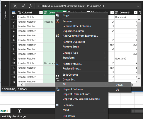
Next, you need to fill in Column1 and Column2 by using Fill > Down.
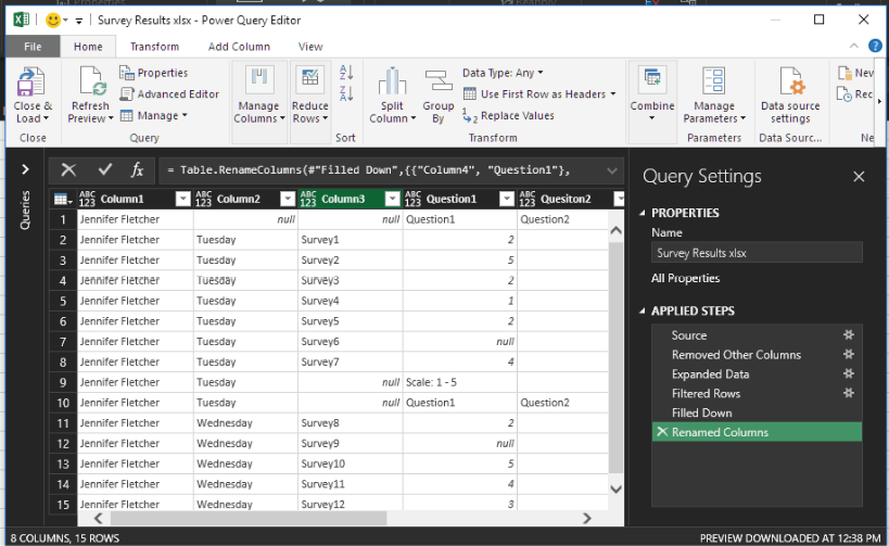
Next, rename Column4, Column5, Column6, and Column7 to Question1, Question2, Question3, and Question4, respectively.

You don’t need the question headers or the rows with Scale: 1 – 5, but you have to be careful about their removal. In Column3, filter out null.
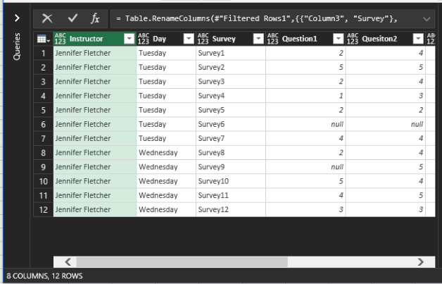
Rename the first three columns Instructor, Day, and Survey.
Now you’re about to get into some serious flattening power. You need two columns:
- Questions
- Scores
That data is in the columns Question1 through Question4, which you’re going to unpivot. Highlight the columns Instructor, Day, and Survey, right-click, and select Unpivot Other Columns.

There you have it! Doesn’t it feel good?
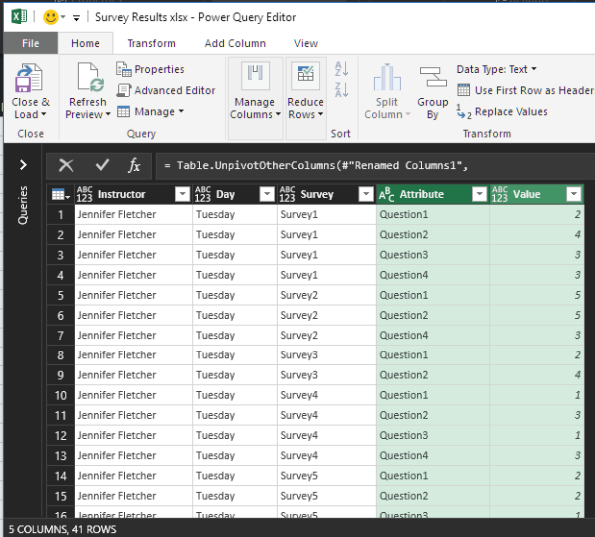
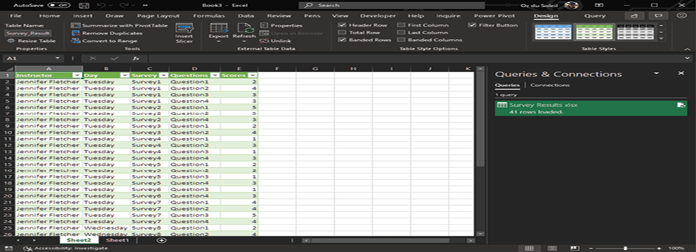
Rename the new columns Questions and Scores and click Close & Load. Now, as shown below, this data is flatted—and it’s useful.
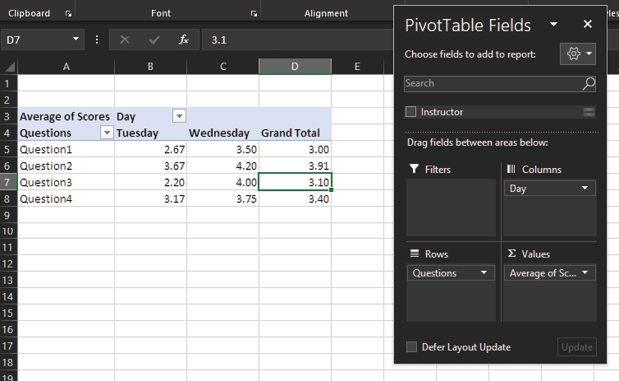
Here’s an example of this data inside a quick-and-easy PivotTable, showing average by day and by question.
A lot of data cleansing needs are unique. You’ll see a particular situation once and never see it again. Therefore, like a blue heron, you must be patient, relax, focus, view the whole situation, and strike when you’re confident that you have a solution. The alternative is to dive into the confusion and possibly make a situation worse.

Many times I’ve seen people faced with complex data cleansing tasks, trying to figure out what to do with data that’s 15,000 rows and 40 columns, spread across 3 workbooks and 12 worksheets. That can involve a lot of scrolling, switching around, highlighting columns, trying this and trying that, getting lost, and thinking too much about the data and not enough about the solution.
My advice? Slow down. Make a small model. Maybe work with 30 rows of data instead of 15,000; start with just enough data to get a fair representation of the problem. Break the task into pieces and get each piece working before integrating the pieces into a final solution.
In closing, here are a few data cleansing tips and review points:
- Never work on your original dataset. You always need a way to get back to the source in case something goes wrong. Make a copy and work on the copy.
- Be aware of the strengths and weaknesses of your data cleansing strategy.
- Accept that data is never ever 100% clean. You have to decide how clean is clean enough.
- Assess the size of your data cleansing project before you dive in.
- To determine how sophisticated your solution needs to be, consider the context and the stakes involved.
- Clarify whether you need a one-and-done solution or a solution that needs to be easily updated or repeated.
- Strategy is key! Excel is loaded with helpful features. But they’re helpful only inside a strategy that clarifies what you are trying to do, what steps you are going to take, and in what order you’re going to take those steps.
- Build a small model of your solution and get it working. Then apply the solution to the larger dataset.
- Take your time. Be patient. Be the blue heron.
