LESSON 8

Transforming Hard Equations into Easier Ones

PURPOSE OF LESSON: To show how one can transform a PDE in u(x,t) into a new (easier) one in a new variable w(x,t). The transformation is generally based on intuition, and in this lesson, the PDEs

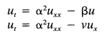
are transformed into the simple heat equation

w_t = α²w_xx

by means of the transformations

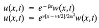
After the transformations are made, the heat equation (the easy one) can be solved for w(x,t), hence,

are the solutions of the original equations (of course, the BCs and the IC must be transformed too).

The reader may get the impression from the last two lessons that the only type of PDE that can be solved by separation of variables is

u_t = α²u_xx

It is true the heat equation is the easiest parabolic PDE to solve by separation of variables, but it is in no way the only equation we can solve by this technique.

As mentioned earlier, as long as the equation is linear and homogeneous, we can separate variables. For example, two-dimensional heat flow inside a circle would be described by the equation

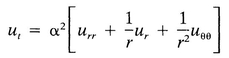
and although it has variable coefficients, it can still be separated into three ODEs.

This lesson will show the reader that sometimes a PDE doesn’t have to be attacked directly but that the original PDE can be transformed into an easier one. In this way, the easier problem can be solved (by separation of variables or some other technique). We now present an example that illustrates this technique.

Transforming a Heat-Flow Problem with Lateral Heat Loss into an Insulated Problem

Consider the following problem:

(8.1)

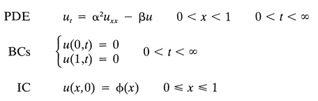
where the term – βu represents heat flow across the lateral boundary (Figure 8.1).

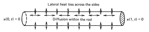
FIGURE 8.1 Heat flow described by u_t = α²u_xx – βu.

The goal of this lesson is to introduce a new temperature w(x,t) in place of u(x,t), so that the PDE in w is simpler than the original one

u_t = α²u_xx – βu

This is a common technique in PDEs, and the transformation is generally based on an intuitive feeling of how the solution of the original PDE behaves. For example, in our problem (8.1), the temperature u(x,t) at any point x₀ is changing as a result of two phenomena

1. diffusion of heat within the rod (due to α²u_xx).
2. heat flow across the lateral boundary (due to – βu).

The important point is that if there were no diffusion within the rod (α = 0), then the temperature at each point x₀ would “damp” exponentially to zero according to

u(x₀,t) = u(x₀,0)e^-βt

By means of this observation, we wonder if we can essentially decompose the temperature u(x,t) of problem (8.1) into two factors

(8.2)

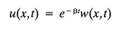
or

Noninsulated temperature = e^-βt (insulated temperature)

where w(x,t) would represent the temperature due to diffusion only. Let’s see what happens if we substitute this expression into problem (8.1); this is a routine calculation (the reader can do it on his or her own), and we arrive at

(8.3)

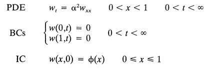
This is exactly the same problem we started with except that now the PDE doesn’t contain – βu; so all we have to do to solve (8.1) is solve the transformed problem (8.3) and then multiply the solution w(x,t) by e^-βt. In this case, we have already solved (8.3) previously by the separation of variables method and found

(8.4)

and, hence, the solution of the original problem (8.1) is

u(x,t) = e^-βtw(x,t)

The following example in the notes is solved by this technique.

NOTES

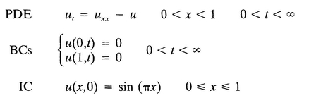
1. To solve the problem

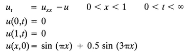
by the preceding strategy, we

1. neglect the convection term – u for the time being.
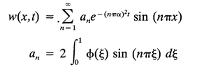
2. solve the initial-boundary-value problem without the term – u to get

   u(x,t) = sin (πx) + 0.5 sin (3πx)

3. multiply this solution by the convection factor e^-βt = e^-t to get the solution
   

2. The diffusion-convection equation

u_t = α²u_xx – vu_x

(v is a constant) can also be transformed to

w_t = α²w_xx

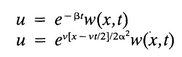
In this case, the transformation is

u(x,t) = w(x,t)

This transformation essentially factors out the part of the solution (exponential factor) that is due to the moving medium. Note that the exponential factor consists of a moving exponential (moving to the right with velocity v/2). The reader will get a chance to use this transformation in the problem set.

PROBLEMS

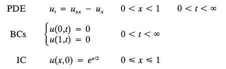
1. Solve the diffusion problem
   
   by transforming it into an easier problem. What does the solution look like? We could interpret this problem as describing the concentration u(x,t) in a moving medium (moving from left to right with velocity v = 1) where the concentration at the ends of the medium are kept at zero (by some filtering device) and the initial concentration is e^x/2. Does your solution agree with this interpretation?
2. Solve the problem
   
   by
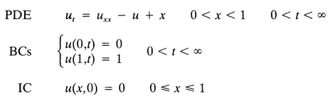
   1. changing the nonhomogeneous BCs to homogeneous ones.
   2. transforming into a new equation without the term – u.
   3. solving the resulting problem.
3. Solve
   
   directly by separation of variables without making any preliminary transformation. Does your solution agree with the solution you would obtain if the transformation

   u(x,t) = e^-tw(x,t)

   were made in advance?

OTHER READING

Nonlinear Partial Differential Equations in Engineering by W. F. Ames. Academic Press, 1965. This text discusses many types of transformations for changing old problems into new ones, so that sometimes even nonlinear problems can be transformed into linear ones.