Multiple linear regression is a powerful and flexible technique that can handle many types of data. However, there are many other of types of regression that are more appropriate for particular types of data or to express particular relationships among the data. We discuss a few of these regression techniques in this chapter. Logistic regression is appropriate when the dependent variable is dichotomous rather than continuous, multinomial regression when the outcome variable is categorical (with more than two categories), and polynomial regression is appropriate when the relationship between the predictors and the outcome variable is best expressed through an equation including polynomial terms (such as x2 or x3). If you are unfamiliar with odds ratios, it would be good to read the section of Chapter 15 covering them before reading this chapter because the odds ratio plays a key role in interpreting the output of logistic regression.
Multiple linear regression may be used to find the relationship between a single, continuous outcome variable and a set of predictor variables that might be continuous, dichotomous, or categorical; if categorical, the predictors must be recoded into a set of dichotomous dummy variables.
Logistic regression is in many ways similar to multiple linear regression, but it’s used when the outcome variable is dichotomous (when it can take only two values). The outcome might be dichotomous by nature (a person is either a high school graduate or she is not) or represent a dichotomization of a continuous or categorical variable. (Blood pressure is measured on a continuous scale, but for the purposes of analysis, people might simply be classified as having high blood pressure or not.) Outcome variables in logistic regression are conventionally coded as 0–1, with 0 representing the absence of a characteristic and 1 its presence. The outcome variable in linear regression is a logit, which is a transformation of the probability of a case having the characteristic in question; you can easily convert logits to probabilities and back, as will be demonstrated.
You might be wondering why you can’t use multiple linear regression with a categorical outcome. There are two reasons:
The assumption of homoscedasticity (common variance) is not met with categorical variables.
Multiple linear regression can return values outside the permissible range of 0–1 (presence or absence).
The logit is also called the log odds for reasons that are clear from its definition. If p is the probability of a case having some characteristic, then the logit for this case is defined as in Figure 11-1.
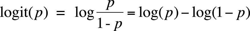
The natural log (base e) is used to convert probabilities to logits.
Apart from having an outcome expressed as a logit, the form of a logistic regression equation with n predictor variables looks very similar to that of a linear regression equation, as can be seen in Figure 11-2.

As with linear regression, we have measures of model fit for the entire equation (evaluating it against the null model with no predictor variables) and tests for each coefficient (evaluating each against the null hypothesis that the coefficient is not significantly different from 0). The interpretation of the coefficients is different, however; instead of interpreting them in terms of linear changes in the outcome, we interpret them in terms of odds ratios (discussed in this chapter and in Chapter 15; note that odds ratios are used frequently in medical and epidemiological statistics).
As with linear regression, logistic regression makes several assumptions about the data:
- Independence of cases
As with multiple linear regression, each case should be independent of other cases, so you should not have multiple measurements on the same person, members of the same family, and so on (if family membership is likely to make cases more related than two cases chosen at random).
- Linearity
There is a linear relationship between the logit of the outcome variable and any continuous predictor. This is tested by creating a model with the logit as outcome and as predictors, each continuous predictor, its own natural logs, and an interaction term of each predictor and its natural log. If the interaction terms are not significant, we can assume the linearity criterion has been met.
- No multicollinearity
As with multiple linear regression, no predictor should be a linear function of other predictors, and predictors should not be too closely related to each other. The first part of this definition is absolute (usually violated only due to the researcher’s absentmindedness, as when including the predictors a, b, and a + b in an equation); the latter is open to interpretation and is assessed through multicollinearity statistics produced during the regression analysis. As discussed in Chapter 10, statisticians disagree on how much of a threat less than absolute multicollinearity presents to a regression model.
- No complete separation
The value of one variable cannot be perfectly predicted by the value(s) of another variable or set of variables. This is a problem that most frequently arises when you have several dichotomous or categorical variables in your model; you can test for it by doing cross-tabulation tables on these variables and checking that there are no empty cells.
Suppose you are interested in factors to health insurance coverage in the United States. You decide to use a random sample of 500 cases from the 2010 BRFSS data set, an annual survey of U.S. adults. (For more on the BRFSS, see Chapter 8.) Insurance coverage is dichotomous; after examining several potential predictors, you decide to use gender (dichotomous) and age (continuous) as predictors. In this data set, 87.4% of the respondents have health insurance, their mean age is 56.4 years (standard deviation 17.1 years), and the respondents are 61.7% female.
Looking at the assumptions for logistic regression, the first is met because we know the BRFSS data is collected by trained researchers following a national sampling plan. To evaluate linearity between the logit and age, we construct a regression model including age, the natural log of age, and the interaction of those two terms. The results are shown in Figure 11-3.
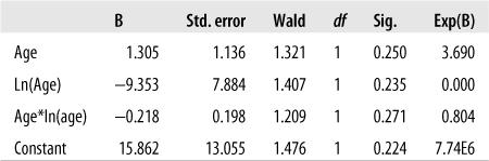
For this analysis, the only thing we are interested in is whether the interaction terms are significant. This is tested by the Wald statistic, a type of chi-square. As we can see from the significance column, the interaction term in this model is not significant, so we can consider the assumption of linearity in the logit met.
We will evaluate multicollinearity by running a linear regression model with multicollinearity diagnostics. We found tolerance values of 0.999 and VIF (variance inflation factor) of 1.001 for both variables, indicating that multicollinarity is not a problem. As discussed in Chapter 10, a standard rule of thumb is that tolerance should not be greater than 10 or VIF less than 0.10. The lack of multicollinearity is not surprising because these data come from a randomized national sample, and over a broad range of ages (18 and older in this case), there is no expected relationship between gender and age.
To check for complete separation, we create a cross-tabulation table between our dichotomous predictor (gender) and outcome (health insurance coverage). The cross-tabulated frequencies are presented in Figure 11-4.
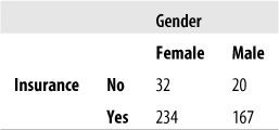
We have no empty cells; in fact, we have no nearly empty cells. The latter can be a problem because although it does not constitute complete separation, it can produce estimates with very high standard errors, hence wide confidence intervals.
To see what complete separation looks like, consider the hypothetical data presented in Figure 11-5.

In this example, all persons who do not have insurance are female. Therefore, if we know that a case does not have insurance, we also know that the case’s gender is female; that is what is meant by complete separation. In practice, complete separation is more likely to occur when you have many categorical predictors (imagine that we included employment status, marital status, and educational level in this model as well) and some of them are sparsely distributed in some categories. A logistic regression model will not run if the data have complete separation, so the best solution is to see whether you can recode the variable. If marital status has six categories (married, widowed, divorced, single never married, living with same-sex partner, living with opposite-sex partner), perhaps you can combine them to produce only two or three categories, each of which includes sufficient cases to avoid the problem of separation. Of course, you need to be able to defend your choice of which categories to combine. For instance, if you could make a case that the most important information is simply whether a person is married versus not married, you should feel free to recode the variable to reflect that information. Even if you don’t have complete separation, it’s wise to avoid a variable with only a few cases in some of its categories because this can produce estimates with extremely wide confidence intervals, as noted earlier.
Having met the assumptions, we continue with the analysis. In logistic regression, overall model fit is evaluated in several ways. First, there is an omnibus test of the model coefficients, testing whether our entire model is better than the null model with no coefficients; the model passes this test with a chi-square statistic (2 df) of 16.686 (p < 0.001). We also get three measures of model fit: the −2 log likelihood, the Cox & Snell R2, and the Nagelkerke R2. The −2 log likelihood is somewhat analogous to the residual sum of squares from a linear regression. It’s hard to interpret the value of the −2 log likelihood by itself, but it is useful when comparing two or more nested models (models in which the larger model includes all the predictors from the smaller model) because a smaller −2 log likelihood indicates better model fit. We can’t compute a Pearson’s R or R2 for a regression model, but two pseudo-R2 statistics are possible: the Cox & Snell and Nagelkerke R2. Both are based on the log likelihood of the model versus the null model; because the range of the Cox & Snell R2 never reaches the theoretical maximum of 1.0, Nagelkerke’s R2 includes a correction, which results in it having a higher value. Both are interpreted the same as the coefficient of determination in linear regression, that is, as the amount of variance in the outcome explained by the model. Because of the correction, Nagelkerke’s R2 generally has a higher value than Cox & Snell’s R2 for a given model. For this model, the −2 log likelihood is 301.230, the Cox & Snell R2 is 0.038, and the Nagelkerke R2 is 0.073.
The coefficients table for this model is presented in Figure 11-6.
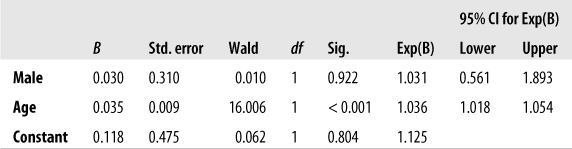
Figure 11-6. Coefficients table for a logistic regression model predicting insurance status from age and gender
We recoded gender into a new variable, Male, with values 0 for female and 1 for male; this is easier to interpret because we don’t have to remember how the category was coded. As with linear regression, the value and significance tests for the constant in logistic regression are usually not our focus of interest. Predictors are evaluated in logistic regression by the Wald chi-square; the significant values are interpreted just like the p-values for any other statistic. In this case, we see that age is a significant predictor of insurance status (Wald chi-square (1 df) = 16.006, p <0.001), whereas male is not significant (Wald chi-square (1 df) = 0.010, p = 0.922). Remembering that we coded insurance status so that 0 = no insurance and 1 = insurance, we see that because the coefficient for age is positive (0.035), increasing age is associated with increasing probability of having insurance.
The Exp(B) column gives the odds ratio for each predictor and the outcome variable, adjusted for all the other variables in the model; the last two columns give the 95% confidence interval for the adjusted odds ratio. If you are unfamiliar with odds ratios, you should read the section covering them in Chapter 15 before proceeding because only a brief explanation will be offered here. An odds ratio is, as the name implies, the ratio of the odds for two conditions. In the case of the first row in this table, the odds ratio for Male is the ratio of the odds of having insurance, if you are male, to the odds of having insurance if you are female. The neutral value for the odds ratio is 1; values higher than 1 indicate increased odds, values lower than 1, decreased odds. Because the odds ratio for male is higher than 1 (1.031), this indicates that in this data set, men have better odds of having insurance than do females. However, this result is not significant, as can be seen from the p-value for the Wald statistic (0.922) and the fact that the 95% confidence interval for the odds ratio (0.561, 1.893) crosses the neutral value of 1. We can therefore say that in a model predicting insurance status from gender and age, gender was not a significant predictor.
Looking at the second line of the table, we see that age is a significant predictor of insurance status in a model also including gender. The adjusted odds ratio is 1.036, and the 95% confidence interval is (1.018, 1.014); note that the confidence interval does not cross 1. The odds ratio for age and male look small (barely higher than 1, in fact), but remember that this is the difference in odds for an increase in age of 1 year; for instance, it is the odds of insurance for someone who is 35 compared to someone who is 34 (adjusted for gender). To find the expected change for a larger number of years, you exponentiate the odds ratio by the number of years. For instance, the predicted change in the odds of having insurance for an age difference of 10 years (adjusted for gender) is:
It’s often useful to report a few hypothetical examples like this along with your results to help your audience understand the importance of variables measured on a continuous scale. The logistic regression equation for this model is:
As noted earlier, though our model is significantly better than the null model at predicting insurance status, it doesn’t explain much of the variance in our data (determined by examining the pseudo-R2 statistics). This is not surprising because there are probably many other variables besides age and gender related to whether a person has insurance; if we were to continue this analysis, we would certainly test the effects of employment and income, for instance. We might also try dichotomizing age to under/over 65 years because we know that virtually everyone over the age of 65 is entitled to insurance coverage under the federal Medicare insurance program. We might also consider running an equation for just people younger than 65 because we don’t expect to see much variation in insurance status for people age 65 and older.
People outside the field of statistics are unlikely to be familiar with the logit, and it’s often better to present results to them in units they understand. For logistic regression, the obvious choice is probabilities. Fortunately, a logistic equation for any set of predictors can be converted to a probability by using the following formula:
Continuing with our previous BRFSS example, we can find the probability of an individual having insurance by plugging his or her X values into our equation and then using that equation in the formula presented earlier. For instance, for a male (X1 = 1) of age 40 (X2 = 40), the predicted logit is:
We then put this value into the equation to predict probability:
If you have a data set that would be suitable for logistic regression, except that the outcome variable is categorical (with more than two categories), it might be a good candidate for multinomial logistic regression. Returning to the BRFSS data, we are interested in what variable predicts health status. Fortunately for us, the BRFSS includes a variable measuring health status on a scale that is commonly accepted and used in the fields of medicine and public health. Often described as self-reported general health, this variable asks people to indicate which of five categories best describes their general health:
Excellent
Very good
Good
Fair
Poor
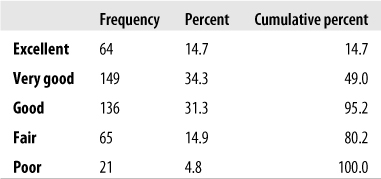
The responses to this question in our sample are displayed in Figure 11-7.
We will use age (continuous) and gender (dichotomous) in a multinomial regression equation to predict self-reported health status. Because we have relatively sparse data in one of our outcome categories, we will do a cross-tabs table with gender to see whether we have empty or nearly empty cells; if so, this would be a problem for the same reason (complete or near-complete separation) discussed in the logistic regression example. The results are shown in Figure 11-8.
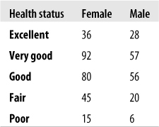
This is mixed news: although we don’t have any empty cells, a cell of size 6 (males in poor health) might give us quite wide confidence intervals. We decide to combine the two lowest categories and proceed with our analysis. We need to choose one of the categories to serve as a reference category for the analysis; the computer algorithm will compare each of the other categories to this one to see whether there is any significant difference among them. We choose the Excellent category.
The model fit information for multinomial logistic regression is similar to that for binomial logistic regression. The −2 log likelihood for this model is 660.234 (this might come in handy if we want to compare the fit of this model to more complex models), and our model predicts significantly better than the null model without predictor variables (χ2 (6 df) = 19.194, p = 0.004). The pseudo-R2 statistics tell us that we aren’t explaining much of the variance (Cox & Snell’s R2 = 0.043, Nagelkerke’s R2 = 0.046), but we’re not surprised: we expect that many more things than gender and age would influence a person’s general health status. We also get likelihood ratio tests, which tell us how model fit changes if one of the predictors is removed. If model fit is significantly lowered (as tested with a chi-square statistic), that means the variable is making a significant contribution to predicting the outcome variable. Data from the likelihood ratio test is presented in Figure 11-9.
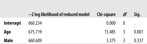
Figure 11-9. Likelihood ratio tests for a multinomial regression model predicting general health status from age and gender
The “reduced model” in each case is the model lacking the variable tested. From this table, we can see that age is a significant predictor of general health status, but gender is not. The intercept is not tested because removing it does not change the degrees of freedom of the model. As we said earlier, a lower −2 log likelihood indicates better fit, so we are not surprised to see a substantial increase in the −2 log likelihood when Age is removed from the model (675.719 vs. 660.234) but very little change (660.608 vs. 660.234) when Male is removed.
The parameter estimates for our full model are presented in Figure 11-10. Note that this is really three models at once because different coefficients are estimated for each of our comparisons (very good versus excellent, good versus excellent, and fair/poor versus excellent).
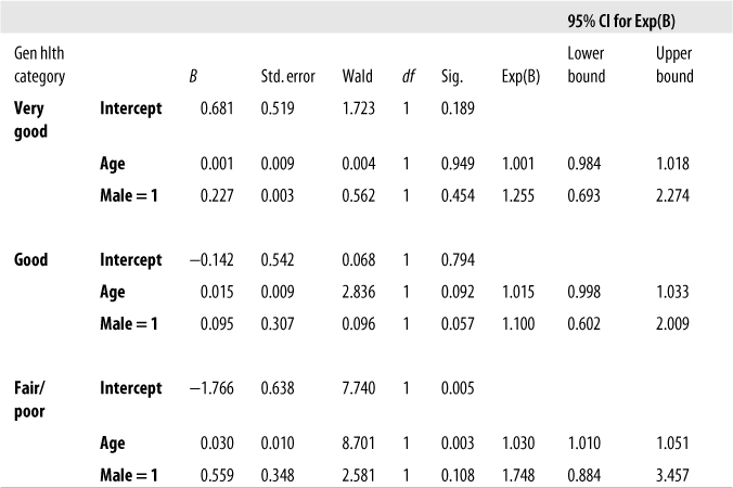
Figure 11-10. Parameter estimates for a multinomial regression model predicting general health status from age and gender
Our misgivings at seeing such low pseudo-R2 statistics are upheld in this model because only one predictor in one of our comparisons is significant: Age for the comparison of Fair/poor versus Excellent health. Because the coefficient is positive (0.030), and the Exp(B) or odds ratio is greater than one, we can see that increased age is associated with increased probability of having Fair/poor versus Excellent health. Note also that the 95% confidence interval for Age in this comparison (1.010, 1.051) does not cross the null value of 1.0, a result expected because the Wald chi-square test is significant for this predictor in this comparison.
So far, you have largely learned about model fitting when the relationship between a DV and one or more IVs is linear, that is, the value of a DV can be predicted by a weighted linear sum of the IVs plus an intercept value. In the two-dimensional plane, such relationships can be viewed as straight lines that have nonzero slope. However, many phenomena have nonlinear relationships, and you need to be able to model these relationships as well. Any relationship that is not entirely linear is, by definition, nonlinear, so any discussion of nonlinear modeling must be very broad indeed. In this section, you learn about two of the most commonly used regression models, which are based on quadratic and cubic polynomials.
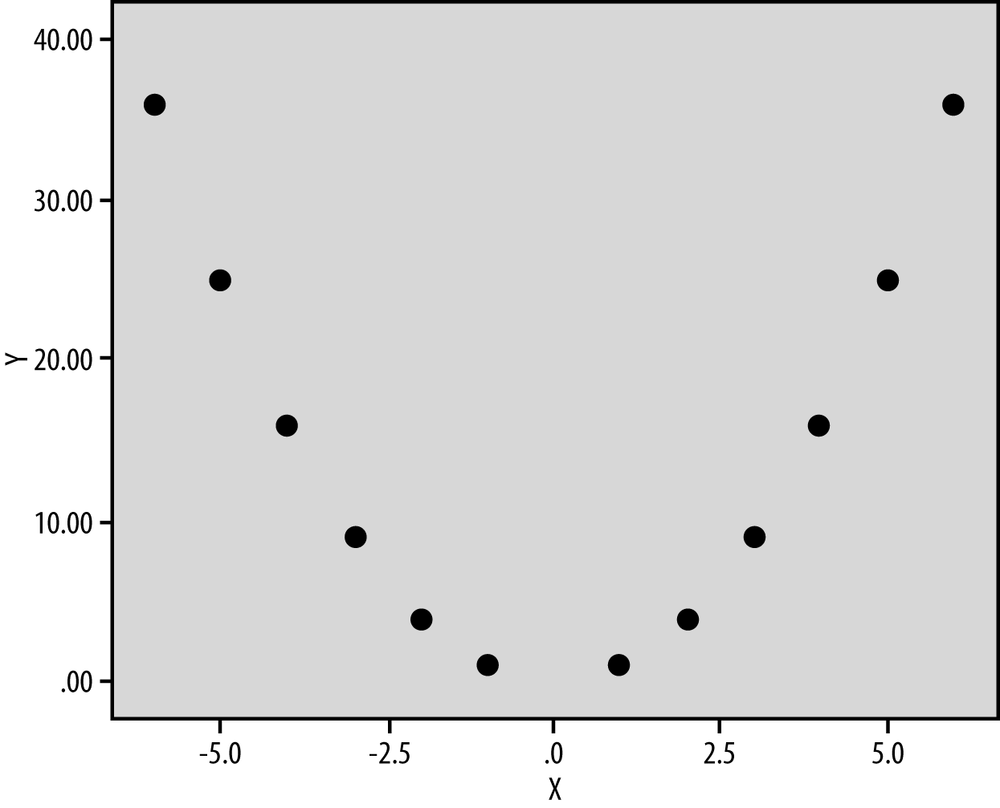
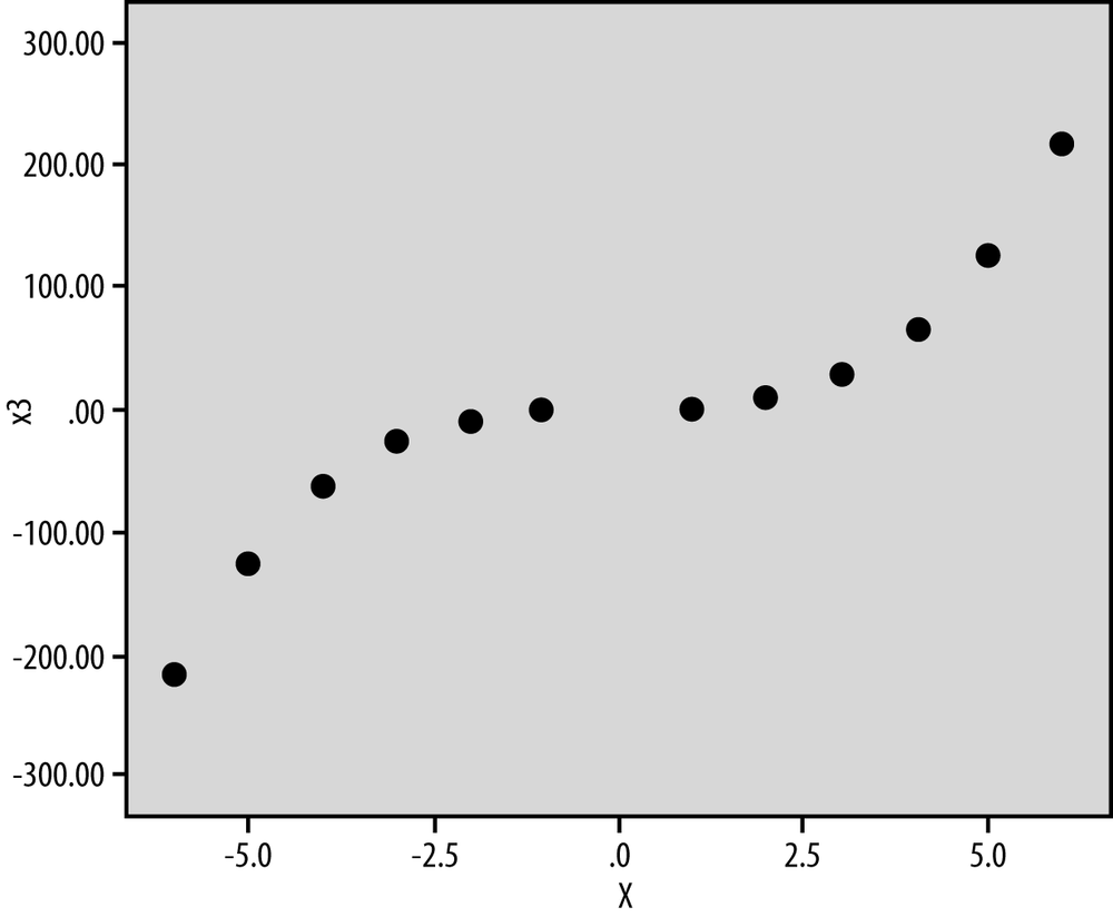
A quadratic model has both a linear and squared term for the IV, whereas the cubic model has a linear, squared, and cubic term for the IV; the principle is that you include all lower order terms as well as the highest order term. Each curve has a number of extreme points equal to the highest order term in the polynomial, so a quadratic model will have a single maximum, whereas a cubic model has both a relative maximum and a minimum. Figure 11-11 shows a quadratic model (Y = X2) and Figure 11-12, a cubic model (Y = X3).
Let’s look at an example from sports psychology. The Yerkes-Dodson Law, first formulated in 1908, predicts a quadratic relationship between arousal (the predictor variable) and performance (the outcome variable). For many athletes, achieving the optimal level of physiological arousal—corresponding to the single maxima of the DV—corresponds to their goal of producing their best possible athletic performance. If athletes are not aroused enough, their performance will be poor; conversely, if athletes are over-aroused, their performance will also be poor.
However, if the relationship between arousal and performance is actually cubic, increasing arousal even further might result in improvements in performance, which would be a contrary prediction to the quadratic model. Polynomial regression can be used to determine the goodness of fit for both the quadratic and cubic models, and the one with the best goodness of fit can be taken as the most accurate description of the relationship between arousal and athletic performance.
Watters, Martin, and Schreter (1997)[3] designed an experiment to determine whether there was a quadratic relationship between caffeine (a drug that produces arousal) and cognitive performance on a battery of tests. The experimental setup required a dose of caffeine to be administered at regular intervals in a single session (6 × 100 mg); this would introduce practice effects and would lead to an increase in performance session to session, independent of arousal. Any residual variation accounted for by a quadratic term would then indicate the underlying relationship between arousal and performance.
You might be wondering why participants in the study were not simply invited back several times to complete the test, with the caffeine dosage randomly assigned on each occasion. The reasoning was ethical; the researchers wanted to observe any adverse reactions at low dosages, which would be impossible on the first trial in a truly randomized design because some of the subjects would be receiving the highest dosage on their first trial, and the researchers wanted to minimize the number of return visits. To obtain a higher degree of experimental control, a repeated measures design was used, in which each participant attended a placebo and treatment session (single blind). If the experimenter noted an adverse reaction, the experiment would be halted. The order of attendance for either the placebo or treatment condition was randomized.
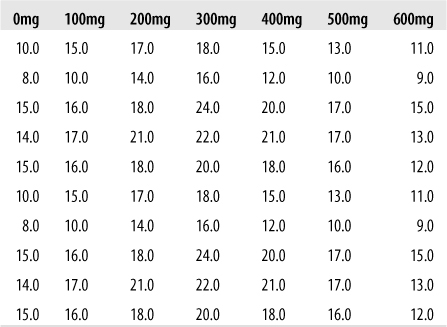
As designed, the experiment had both a within-subjects and between-subjects comparison, with the former showing the dose-response relationship and the latter confirming that the dose-response relationship observed was not the product of chance (or practice). Only the within-subjects analysis is shown here. The analysis proceeds by adding terms progressively into the model, starting with caffeine, followed by the square and cube of caffeine. Figure 11-13 shows some sample data that may be obtained in this type of experiment.
For the linear model Y = β0 + β1X1 + e, where Y is performance and x is caffeine, there was virtually no relationship between the two variables: R2 = 0.001, and the F-statistic also showed that the coefficient for caffeine was not significantly different from 0 (F(1, 68) = 0.097, p = 0.757).
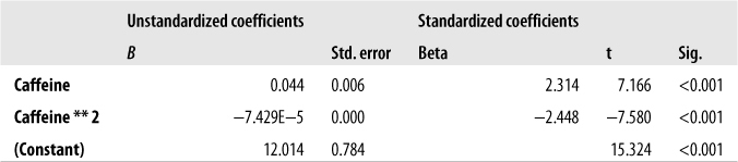
For the quadratic plus linear model, Y = β0 + β1X1 + β2X12 + e for the same variables found a significant relationship between caffeine and performance. For this model, R2 = 0.462, F(2, 67) = 28.81, and p < 0.001. The coefficients table for this model, Figure 11-14, shows that both the linear and quadratic terms made a significant contribution to the model fit, with a strongly linear effect accompanied by a negative quadratic term. The relative contribution that both terms make to the model, as demonstrated by the absolute value of their beta coefficients, is comparable (βlinear = 2.314 versus βquadratic = −2.448).
The cubic plus quadratic plus linear model Y = β0 + β1X1 + β2X12 + β3X13 + e did not explain a significant additional amount of variation in performance, and the coefficient for the cubic term was not significant, confirming that the linear and quadratic relationship model best explains the relationship between caffeine consumption and athletic performance.
One of the more amazing features of modern statistical computing packages is that you can automatically specify and perform any number of tedious statistical tests at the click of a button. This ability to run many models quickly can be useful if you are simply exploring the data, or if your a priori hypotheses have failed to meet expectations and you are trying to figure out what is actually going on in the data. However, many statisticians frown on building models based purely on a given data set, deeming it “going on a fishing expedition” and, when nonlinear regression is involved, arbitrary curve-fitting. We discussed the dangers of mechanical model-building in Chapter 10, but the cautions apply even more here because you are not simply adding and subtracting predictor variables but also changing their form. However, this type of model building is acceptable in some fields, so if that is the case in your workplace or school, there’s no reason you shouldn’t take advantage of all the possibilities offered by modern computer packages. Some statistical packages allow you to request that all possible linear and nonlinear relationships between two variables be calculated, and then you can simply select the one that does the best job of explaining the data.
If you’re going to engage in this type of model fitting, you should be aware of the dangers inherent in the process. We illustrate these with a simple example. Imagine that you are a nutritionist interested in the relationship between smoking and blood pressure, with the results obtained from a small study shown in Figure 11-15. You know that there is a relationship between the two, but as an expert witness in a court case, you are under pressure to prove the strongest possible link between the two variables. Some of the data, showing the diastolic blood pressure and daily cigarette consumption for the first few cases, is shown in Figure 11-15.
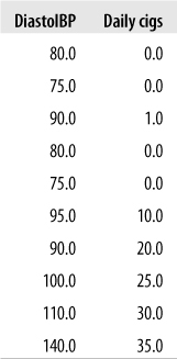
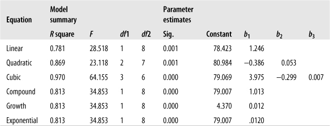
Summary results from a few models (with diastolic blood pressure as the outcome, and daily cigarettes smoked as the predictor) are displayed in Figure 11-16. As you can see from Figure 11-16, there are many types of relationships two variables can have besides linear. Even more surprising, a model including linear and quadratic terms explains 97% of variability in diastolic blood pressure. No one has ever reported a cubic relationship between the two variables before, so you think you have discovered a very convincing argument.
Do the R2 values computed by such an approach have any real meaning? Yes and no; one real risk with fishing expeditions is overfitting. This means your data fits your data set too well and explains the random variation in it as well as the significant relationships. Because the purpose of inferential statistical analysis is to find results that will generalize to other samples drawn from the same population, overfitting defeats the whole purpose of conducting the analysis in the first place. You might have a model that fits your particular data set remarkably well, but it won’t necessarily fit any other data set, so it hasn’t produced any useful knowledge for your field.
The best protection against overfitting is to build your models based on theory. If you decide to use mechanical procedures to build your model, you should test it across multiple samples to be sure you are modeling major relationships within the data instead of random noise. If only limited samples are available, such as in destructive testing environments, resampling techniques such as bootstrapping and the jackknife may be employed; these are discussed in the Efron book listed in Appendix C.
Problem
You are comparing two nested logistic regression models (models in which the larger models include all the predictor variables included in the smaller models). Model A has a −2 log likelihood of 200.465; Model B has a −2 log likelihood of 210.395. Which model fits the data better?
Solution
Model A has the better fit; when comparing two nested models, the model with the smaller −2 log likelihood fits the data better.
Problem
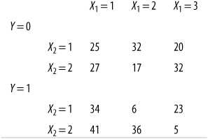
You are planning a logistic regression analysis, using one dichotomous and one categorical predictor. The following table presents cross-tabulation results for the Y variable and the two predictors (X1 and X2). Do any alarm bells go off when you read this table? If so, how would you fix the problem?
Solution
Although there are no empty cells, two are sparsely populated (with 6 and 5 cases, respectively), which might result in wide confidence intervals. If possible (and theoretically defensible, based on the meanings of the categories for variable X1), the best solution may be to combine the second and third categories for this variable.
Problem
You have conducted a logistic regression analysis to predict the probability of high school students becoming dropouts, using their GPA and gender as predictors. This is your regression equation:
| Logit(p) = 4.983 + 1.876(male) −2.014(GPA) + e |
| Dropout (the Y variable) is coded so 1 = dropped out, 0 = not dropped out. |
| GPA is a continuous variable ranging from 0.00 to 4.00. |
| Male (the gender variable) is coded so 0 = female and 1 = male. |
What is the predicted probability of dropout for a female with a 3.0 GPA?
Solution
To calculate this probability, plug the values for female and GPA into the logistic regression equation and then use the following formula to calculate the predicted probability of dropout:
The predicted logit is:
The predicted probability of dropping out is:
Problem
Continuing with the problem of predicting who will drop out of high school, you decide to add another variable to the equation: whether the student’s mother graduated from high school (coded so 0 = no, 1 = yes). After doing the appropriate data checks, you run the equation, which produces the coefficients and significance tests shown in Figure 11-17. This model is significantly better than the null model in predicting high school dropouts (chi-square (3) = 28.694, p < 0.001); the value for the Cox & Snell R2 is 0.385 and, for the Nagelkerke R2, 0.533.
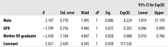
Figure 11-17. Coefficients for a logistic regression equation predicting the high school dropout from gender, GPA, and mother’s education
Interpret the information in this table, including specifying which predictors are significant, in which direction, and what the Exp(B) column and its 95% confidence interval means.
Solution
All the predictor variables in this model are significantly related to the probability of a student dropping out of high school. Males are more likely than females to drop out (B = 2.107; Wald chi-square (1) = 7.495, p = 0.006). Higher GPA predicts a lower probability of dropping out (B = −1.599; Wald chi-square (1) = 4.466, p = 0.035), as does having a mother who graduated from high school (B = −2.430; Wald chi-square (1) = 4.867, p = 0.028).
The Exp(B) column presents the adjusted odds ratios for each of the predictor variables. As expected, male gender has an odds ratio greater than 1 (8.224), indicating that males are more than 8 times as likely as females to drop out, after adjusting for GPA and mother’s education; the 95% confidence interval for male gender is (1.819, 37.170). The odds ratios for GPA and having a mother who graduated from high school are less than 1, indicating that a higher GPA or a mother who is a high school grad are associated with a lower probability of dropping out. The odds ratios and the 95% confidence intervals are 0.202 (0.046, 0.890) for GPA and 0.088 (0.010, 0.766) for having a mother who graduated from high school. Note that none of the confidence intervals cross the neutral value of 1; this is expected because all the predictors are significant.
[3] Watters, P.A., Martin, F., & Schreter, Z. (1997). “Caffeine and cortical arousal: The nonlinear Yerkes-Dodson Law.” Human psychopharmacology: clinical and experimental, 12, 249–258.