You might wonder what a chapter on data management is doing in a book about statistics. Here’s the reason: the practice of statistics usually involves analyzing data, and the validity of the statistical results depends in large part on the validity of the data analyzed, so if you will be working with statistics, you need to know something about data management, whether you will be performing the management tasks yourself or delegating them to someone else.
Oddly enough, data management is often ignored in statistics classes, as well as in many offices and labs; some professors and project managers seem to believe that data will magically organize into a usable form without human intervention. However, people who work with data on a daily basis have quite a different view of the matter. Many describe the relationship of data management to statistical analysis by invoking the 80/20 rule, meaning that on average 80% of the time devoted to working with data is spent preparing the data for analysis, and only 20% of the time is spent actually analyzing the data. In my view, data management consists of both a general approach to the problem and the knowledge of how to perform a number of specific tasks. Both can be taught and learned, and although it’s true that some people can pick up this knowledge on an informal basis (through the college of hard knocks, so to speak), there is no good reason to leave such matters up to chance. Instead, it makes more sense to treat data management as a skill that can be learned like any other, and there’s no reason not to take advantage of the collective wisdom of those who have gone before you.
The quality of an analysis depends in part on the quality of the data, a fact enshrined in a phrase that originated in the world of computer programming: garbage in, garbage out, or GIGO. The same concept applies to statistics; the finest statistician cannot produce valid results if the data is a mess. The process of data collection by its nature is messy, and seldom does a data file arrive in perfect shape and ready for analysis. This means that at some point between data collection and data analysis, someone has to get her hands dirty working directly with the data file, cleaning, organizing, and otherwise getting it ready for analysis. There’s usually no mystery about what needs to be done during this process, but it does require a systematic approach guided by knowledge of the data and the uses to which it will be put as well as an inquisitive attitude informed by common sense.
GIGO has another meaning that applies equally well to statistical analysis: garbage in, gospel out. This phrase refers to the distressing tendency of some people to believe that anything produced by a computer must be correct, which we can extend to the equally distressing belief that any analytic results produced using statistical procedures must be correct. Unfortunately, there’s no getting around the need for human judgment in either case; computers and statistical procedures can both produce nonsense instead of valid results if the data provided to them is faulty. To take an elementary example, the fact that you can calculate the mean and variance of any set of numbers (even if they represent measurements on a nominal or ordinary scale, for instance) does not mean that those numbers are meaningful, let alone that they provide a reasonable summary of the data. The burden is on the analyst to provide correct data and to choose an appropriate procedure to analyze it because a statistical package simply performs the operations you request on the data you provide and cannot evaluate whether the data is accurate or the procedures appropriate and meaningful.
If your interest is restricted to learning statistical procedures, you might want to skip this chapter. Similarly, if you have no practical experience working with data, this chapter might seem entirely abstract, and you might want to skim or pass over it until you’ve actually handled some data. On the other hand, in either circumstance, you might still find having a basic understanding of what is involved in the process of data management useful and want to become aware of what can happen when it isn’t done correctly. In addition, it’s always good to know more than you need to for your immediate circumstances, particularly given that career change is a salient feature of modern life. You never know when a little knowledge of data management will give you an edge in a job interview, and reading this chapter should help you speak convincingly on topic, giving you an advantage over many other candidates. In addition, if in the future data management should become one of your responsibilities, the information in this chapter will start you off with a good understanding of why data management is important and how it is done.
Because many methods and computer programs are used to collect, store, and analyze data, it’s impossible to write a chapter spelling out how to carry out data management procedures that will work in all circumstances. For that reason, this chapter focuses on a general approach to data management, including consideration of issues common to many situations as well as a generalized process for transforming raw data into a data set ready for analysis.
If I had to give one piece of advice concerning data management, it would be this: assume nothing. Don’t assume that the data file supplied to you is the file you are actually supposed to analyze. Don’t assume that all the variables transferred correctly when the file was translated from one program to another. (Volumes could be written on this subject alone, and every version of any software seems to include a new set of problems.) Don’t assume that appropriate quality control was exercised during the data entry process or that anyone else has examined the data for out-of-range or otherwise impossible values. Don’t assume that the person who gave you the project is aware that an important variable is missing for 50% of the cases or that another variable hasn’t been coded in the way specified by the codebook. Data collection and data entry are activities performed by human beings who have been known to make mistakes now and then. A large part of the data management process involves discovering where those mistakes were made and either correcting them or thinking of ways to work around them so the data can be analyzed appropriately.
Without getting too carried away with the military metaphor, it is true that efficient data management for a large project requires establishing a structure or hierarchy of people who are responsible for different aspects of the process. Equally important, everyone involved in the project should know who is authorized to make what decisions so that when a problem arises, it can be resolved quickly and reasonably. This might sound like simple common sense, but in fact, it is not always exercised in practice. If the data entry clerk notices that data is coming in with lots of variables missing, for instance, he should know exactly who to report this problem to so it can be corrected while the project is still in the data collection phase. If an analyst finds out-of-range values during initial inspection of the data file, she should know who is authorized to make the decision about what to do with those values so they can be corrected or recoded before the main analysis begins. Make it difficult for such issues to be resolved, and the staff is likely to impose its own ad hoc solutions or give up trying to deal with them, leaving you with a data set of uncertain quality.
The codebook is a classic tool of research, and the principle of the codebook applies to any project that involves collecting and analyzing data. The codebook is simply a means to collect and organize important information about a project. Sometimes the codebook is a physical object such as a spiral notebook or a three-ring binder, and sometimes it is an electronic file (or a collection of files) stored on a computer. Some projects use a hybrid system in which most of the codebook information is stored electronically, but some or all of it is also printed and kept in a binder. The bottom line is that it doesn’t matter what method you choose as long as the vital information about the project and the data set is reliably recorded and stored for future reference.
At a minimum, the codebook needs to include information in the following categories:
The project itself and data collection procedures used
Data entry procedures
Decisions made about the data
Coding procedures
Details about the project include its goals, timeline, funding, and some statement of the personnel involved (original plus any changes) and their duties. Information about data collection procedures includes when the data was collected, what procedures were used, whether any sort of quality control was used, and who actually collected the data. If a form like a questionnaire was used, a copy should be included in the codebook, as should any instructions given to the data collection team. Decisions made about the data include matters such as definitions of outliers (a case whose value is far different from others in the data set) or other unusual values, details about any cases that were excluded from analysis and why, and any imputation or other missing data procedures that were followed. Information about coding procedures include the meaning of variables and their values, how and why variables were recoded, and the codes and labels applied to them.
Recording information about data entry procedures is particularly important when data is collected in one medium, for instance by using paper questionnaires, and analyzed in another, such as in an electronic file. However, even if a CATI (computer-assisted telephone interviewing) system or other method of electronic data collection was used, the codebook should explain how the individual files were collected and transferred. Usually, electronic file transfer works smoothly, but not always, and every time a file is transferred it creates an opportunity for a data file to become corrupted. If the file for analysis is discovered to be corrupted, it might be necessary to trace backward through the transfer process to determine what happened and to develop a way to correct it. Information about the training of data entry personnel and any quality control methods used (such as double entry of a sample of the data) should also be recorded.
In my experience, companies whose data consists of the records of their day-to-day business operations do a better job of documentation than academics and others working on small projects with data collected specifically for each project. Several factors are involved here. One is that when data collection and storage processes are ongoing, it is relatively easy to establish a set of procedures and follow them. Another is that large companies that deal with data on a regular basis often have a staff of people assigned specifically to manage that data, and those people receive special training relevant to their job. In academia, the opposite situation is often the rule; a lab might be involved in a number of projects, each involving different data and each data set having its own set of quirks. Matters are often complicated by the fact that the responsibilities of collecting and organizing this data can be relegated to undergraduates with minimal experience or training or to PhDs or MDs who are subject matter experts but unfamiliar with (and possibly uninterested in) the day-to-day issues of data management.
The main reason you need a codebook or its equivalent is to create a repository of information about each project and its data, so that people who join a project or analyze the data long after the collection process has ceased know what the data is and how to interpret it. The existence of a reliable codebook is also helpful for people who have been involved in a project from the start because no one’s memory is perfect, and it’s easy to forget what decisions were made six months or two years ago. Having the codebook information easily accessible is also a great time-saver when it’s time to write up your results or when you need to explain the project to a new analyst.
Seldom is data ready to be analyzed exactly as it has been collected. Before analysis begins, someone needs to examine the data file and make decisions about problems such as out-of-range values and missing data. All these decisions should be recorded, as well as the location of each version of the file. An archived version of the original data file should be stored somewhere it can’t be changed in case you want to reverse a coding decision later or in case the edited file becomes corrupt and has to be recreated. It’s also sensible to store versions of the file after each major round of editing in case you decide that decisions made in rounds 1, 2, 3, and 5 were valid but not those of round 4. Being able to go back to version 3 of the data file saves you from having to process the original version from scratch. The number of variables and cases in each version of the file, as well as the file layout, should also be recorded. Every time a file is transferred, you need to confirm that the right number of cases and variables appear in the new version, and the file layout is useful when you need to refer to variables by position rather than name (for instance, if the last variable in the file didn’t survive a transfer). If any method such as imputation is used to deal with missing data, details on the method used and how this changed the data file should also be recorded.
Records of the coding procedures used for a project will probably occupy the largest part of your codebook. Information that should be recorded here includes the original variable names, labels added to variables and data values, definitions of missing value codes and how they were applied, and a list of any new variables and the process by which they were created (for instance, by transforming an existing variable or recoding a continuous variable into categories).
There are many ways to store data electronically, but the most common format is the rectangular data file. This format should be familiar to anyone who has used a spreadsheet program such as Microsoft Excel, and although statistical packages such as SAS and SPSS can read data stored in many formats, the rectangular data file is often used because it facilitates the exchange of data among different programs.
The most important aspect of a rectangular data file is the way it is laid out. For data prepared for statistical analysis, the usual convention is that each row represents a case and each column represents a variable. The definition of a case depends partly on the analysis planned and involves the concept known as the unit of analysis (discussed further in the sidebar Unit of Analysis). Because sometimes data about one case is recorded on multiple lines or data about multiple cases is recorded on a single line, some prefer to say that one line represents one record rather than one case.
Figure 17-1 displays an excerpt of data from the General Social Survey of 1993, a nationally representative survey that has been conducted by the National Opinion Research Center at the University of Chicago almost every year since 1972. Each line holds data collected from one individual, identified by the variable id in the first column. Each column represents data pertaining to a particular variable. For instance, the second column holds values for the variable wrkstat, which is the individual’s response to a question about her work status, and the third column holds values for the variable marital, which is the individual’s response to a question about her marital status.
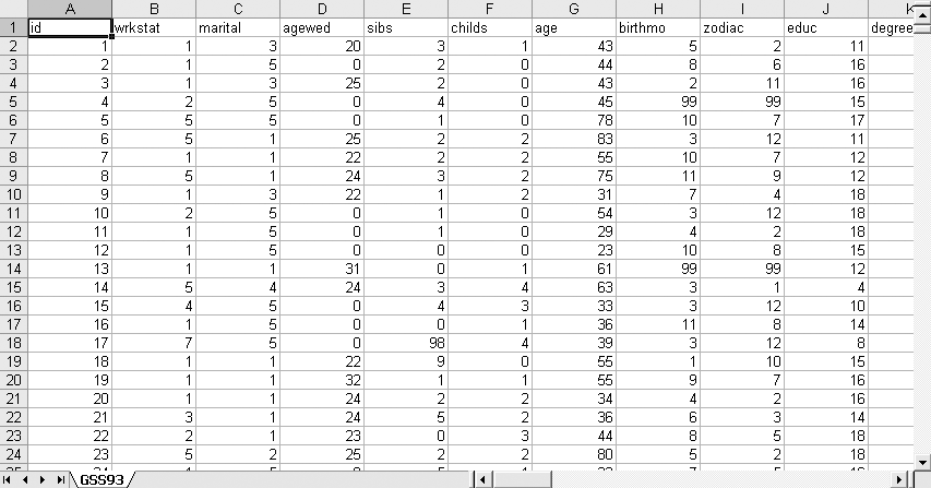
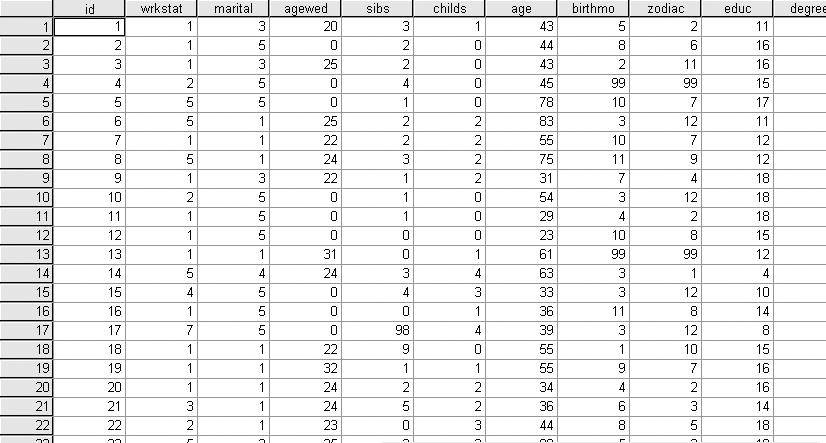
Figure 17-2 shows the same excerpt from the same data file in SPSS. The chief difference is that in Excel, the first row stores variable names (id, wrkstat, etc.), whereas in SPSS, variable names are linked to the data but do not appear as a line in the data file. This difference in storage procedure means that when moving a data file from Excel to SPSS, there will appear to be one fewer case in SPSS than in Excel, but in fact, the difference is due to the row of data names used in Excel but not in SPSS. Transferring data from one program to another often involves this type of quirk, so it’s good to know something about each system or program through which the data will pass.
Although other data arrangements are possible in spreadsheets, such as placing variables in rows and cases in columns, these methods are generally not used for data that will be imported into a statistical program. In addition, although spreadsheets allow for the inclusion of other types of information beyond data and variable names, such as titles and calculated fields, that information should be removed before the data is imported into a statistical program.
The main consideration when setting up a system of electronic data storage should be to facilitate whatever you plan to do with it. In particular, remember that whatever program or statistical package you intend to use to analyze this data (Minitab, SPSS, SAS, or R) has specific requirements, and it is your responsibility to provide the data in a form that your chosen program can use. Fortunately, many statistical analysis packages provide built-in routines to transform data files from one format to another, but it remains the responsibility of the data manager and/or statistical analyst to determine which format is required for a particular procedure and to get the data into that format before beginning the analysis.
Even if a project’s data will ultimately be analyzed using a specialized statistical analysis package, it is common to collect and/or enter the data by using a different program such as Excel, Microsoft Access, or FileMaker. These programs can be simpler to use for data entry than a statistical package, and many people have them installed on their computers anyway (particularly Excel), limiting the number of licenses of specialized statistical software that must be purchased. Excel is a spreadsheet, and Access and Filemaker are relational databases. All three can open electronic files from other programs and write files that can be opened by other programs, making them good choices if data will be transferred among programs. In addition, all three can also be used to inspect the data and compute elementary statistics.
For small projects with simple data sets, a spreadsheet can be completely adequate for data entry. The advantage of spreadsheets is their simplicity; you can create a new data file simply by opening a new spreadsheet and typing the data into the window, and the entire data set can be contained in a single document. Beginners find spreadsheets easy to use, and the spreadsheet format encourages entering data in the rectangular data file form, facilitating data sharing among programs.
Relational databases can be a better choice for larger or more complex projects. A relational database consists of a number of separate tables, each of which looks similar to a spreadsheet page. In a well-designed database, each table holds one particular type of data, and the tables are linked by key variables. This means that within the database, data for one case (for instance, for one person) might be contained in many separate, specialized tables. A student database might have one table for student home addresses, one for birth dates, one for enrollment dates, and so on. If data needs to be transferred to a different program for analysis, the relational database program can be used to write a rectangular data file that contains all the desired information in a single table. The chief advantage of a relational database is efficiency; data need never be entered more than once, and multiple records can draw on the same data. In the school example, this would mean that several siblings could draw on the same home address record, but in a spreadsheet, that information would have to be entered separately for each child, raising the possibility of typing or transcription errors.
Let’s assume you have just been sent a new data file to analyze. You have read the background information on the project and know what type of analysis you need to perform, but you need to confirm that the file is in good shape before you proceed. In most cases, you will need to answer the following questions (at least) before you begin to analyze the data. To answer these questions, you must open the data file and, in some cases, run some simple procedures such as creating frequency tables (discussed in Chapter 4). Some statistical packages have special procedures to aid in the process of inspecting a new data file, but almost any package allows you to perform most of the basic procedures required. However, you might also wish to consult one of the specialized manuals that explain the specific data inspection and cleaning techniques available with particular statistical packages; several such books are listed in Appendix C.
The following are some basic questions for a new data file:
How many cases are in the file?
How many variables are in the file?
Are there any (unintended) duplicate cases?
Did the variable values, names, and labels transfer correctly?
Is all the data within reasonable range?
How much data is missing and in what patterns?
You should know how many cases are expected to be in the data file you received. If that does not match up with the number actually in the file, perhaps you were sent the wrong file (which is not an uncommon occurrence), or the file was corrupted during the transfer process (also not uncommon). If the number of cases in your file does not match what you were expecting, you need to go back to the source and get the correct, uncorrupted file before continuing in your investigation.
Assuming the number of cases is correct, you also need to confirm that the correct number of variables is included in the file. Aside from being sent the wrong data file, missing variables can also be due to the file becoming corrupted during transfer. One thing in particular to be aware of is that some programs have restrictions on the number of variables they will handle; if so, you need to find another way to transfer the complete file. If this is not possible, another option is to create a subset of the variables you plan to include in your analysis (assuming you won’t be using all the variables in the original file) and just transfer that smaller file instead. A third possibility is to transfer the file in sections and then recombine them.
Assuming you have a file with the correct number of cases and variables, you next want to see whether it contains any unintended duplicate cases. This requires communication with whoever is in charge of data collection on the project to find out what constitutes a duplicate case and whether the data includes a key variable (see the upcoming sidebar Unique Identifiers if this term is unfamiliar) to identify unique cases. The definition of a duplicate case depends on the unit of analysis. For instance, if the unit of analysis is hospital visits, it would be appropriate for the same person to have multiple records in the file (because one person could have made multiple hospital visits). In a file of death records, on the other hand, you would expect only one record per individual. Different methods are available to identify duplicate records, depending on the software being used as well as the specifics of the data set. Sometimes it is as simple as confirming that no unique identifier (for instance, an ID number) appears more than once, whereas in other cases, you might need to search for multiple records that have the same values on several or all variables.
Checking that variable values, names, and labels are correct is the next step in inspecting a data file. Correct transfer of data values is the most important issue because names and labels can be recreated, but the data must be correct, and many unexpected things can happen to data in the file transfer process. Among the things you should check are correct variable type (sometimes numeric variables are unexpectedly translated to string variables or vice versa; see the following section on string and numeric variables), length of string variables (which are often truncated or padded during transfer), and correct values, particularly for date variables. Most statistical packages have a way to display the type, length, and labels associated with each character, and this should be used to see that everything transferred as expected.
Variable names can change unexpectedly during the file transfer process due to different programs having different rules about what is allowable in a variable name. For instance, Excel allows variable names to begin with a number, but SAS and SPSS do not. Some programs allow names up to 64 characters in length, whereas others truncate names at 8 characters, a process that can result in duplicate variable names or the substitution of generic names such as var1. Although data can usually be analyzed no matter how the individual variables are named, odd and nonmeaningful names impose an extra burden on the user and can make the analytical process less efficient. Some advance planning is in order if data will be shared among several programs. In particular, someone needs to confirm the naming conventions for each program whose use is anticipated and to create variable names that will be compatible with all the programs that will be used.
Variable and value labels are a great convenience when working with a data file but often create problems when files are moved from one program or platform to another. Variable labels are text phrases attached to a variable that provide one way to work around name length restrictions. For instance, the variable wrkstat in the GSS example could be assigned the label “Work status in the previous six months,” which does a much better job of conveying what the variable actually measures. Value labels are assigned to variable labels but are assigned to the values of individual variables. Continuing with the previous example, for the variable wrkstat, we might assign the label “Full-time employment” to the value 1, “Part-time employment” to the value 2, and so on. Convenient as variable and value labels might be, they often don’t transfer correctly from one program to another because each program stores this information differently. One solution, if you know that the data will be shared across several platforms and/or programs, is to use simple variable names such as v1 and v2 and simple numeric codes for values (0, 1, 2, etc.), and write a piece of code (a short computer program) to be run on each platform or program that assigns the variable and value labels.
The next step is to examine the actual values in the data set and see whether they seem reasonable. Some simple statistical procedures (such as calculating the mean and variance of numeric variables) can help confirm that the data values were transferred correctly (assuming you have the values for mean and variance for the data set before it was transferred). Date variables should be checked particularly carefully; they are a frequent source of trouble because of the different ways dates are stored in different programs. Generally, the value of a date is stored as a number reflecting the number of units of time (days or seconds) from a particular reference date. Unfortunately, each program seems to use a different reference date, and some use different time units as well, with the consequence that date values often do not transfer correctly from one program to another. If date values cannot transfer correctly, they can be translated to string variables, which can then be used to recreate the date values in the new program.
Even if you have confirmed that the file transferred correctly, there might still be problems with the data. One thing you have to check for is impossible or out-of-range variables, which is easily done by looking at frequencies (or the minimum and maximum values if a variable has many values) to see whether they make sense and match with the way the variable was coded. (Frequency tables are discussed in Chapter 4.) If a data file is small, it might also be feasible simply to sort each variable and look at the largest and smallest values. A third option, if you are using Excel, is to use the data filter option to identify all the values for a particular variable. Typical problems to watch out for include out-of-range data (someone with an age of 150 years), invalid values (3 entered in response to a question that has only two valid values, 0 and 1), and incongruous patterns (newborn infants reported as college graduates). If you find unusual values or obvious errors after confirming that the file transferred correctly, someone will have to make a judgment call about how to deal with these problems because once you begin statistical analysis, the program will treat all the data you supply for an analysis as valid.
The final step before beginning an analysis is to examine the amount of missing data and its patterns. Your first goal is to discover the extent of the missing data, a task that can be accomplished using frequency procedures. The second is to examine the patterns of missing data across multiple variables. For instance, is data frequently missing on particular sets of variables? Are there some cases with lots of missing data, whereas others are entirely or primarily complete? Does the file include information about why data is missing (for instance, because a person declined to provide information versus because a question did not apply to her) and, if so, how is that information coded? Finally, you need to decide how you will deal with the missing data, a topic that is discussed later in this chapter.
One distinction observed in most electronic data processing and statistical analysis systems is the difference between string and numeric variables, although they might use different names for the concepts. The values stored in string variables, which are also called character or alphanumeric variables, can include letters, numbers, blanks, and symbols such as #. (The specific characters allowed vary across different systems.) String variables are stored as a series of coded values; the coding systems most commonly used are EBCDIC (Extended Binary Coded Decimal Interchange Code) and ASCII (American Standard Code for Information Interchange). Because string variables are stored as a series of codes, each with a defined position within the variable, certain procedures are possible that refer to the position of the characters. For instance, many programming systems allow you to perform tasks such as selecting the first three characters of a string variable and storing it in a new string variable.
Numeric variables are stored as values rather than as the characters that are used to write those values. They may be used in mathematical and statistical procedures such as addition and subtraction, whereas string variables may not. In some systems, certain symbols such as the decimal point, comma, and dollar sign are also allowed within numeric variables. One point to be aware of is that the values of string variables coded with leading zeroes (0003) will lose those leading zeroes (3) if converted to numeric variables.
The specific method used to store the values of numeric variables differs across platforms and systems, as does the precision with which those values are stored. You should be aware that when transferring electronic files from one system to another, the variable type can change, or certain values that were read as valid in the first system might be recoded as missing in the second. This is a problem that must be handled on a file-by-file basis; the specific problems that occur when transferring files from Excel to SPSS, for instance, might be different from those that occur when transferring files from Access to SAS.
Missing data is a common problem in data analysis. Despite the ubiquity of missing data, however, there is not always a simple solution to deal with this problem. Instead, a variety of procedures and fixes is available, and analysts must decide what approach they will take and how many resources they can afford to dedicate to the problem of missing data. This discussion can only introduce the main concepts concerning missing data and suggest some practical fixes. For a more in-depth and academic discussion, see the classic text, Statistical Analysis with Missing Data, by Little and Rubin (Wiley) listed in Appendix C.
Data can be missing for many reasons, and it is useful if the reasons are recorded within the data set. Often, programs allow you to use specific data codes to differentiate among different types of missing data, using values such as negative numbers that cannot appear as true values for the variable in question. An individual completing a survey might refuse a particular question, might not have the information requested, or the question might simply not apply to him. These three types of responses could be assigned different codes (say, −7, −8, and −9) and the meaning of each code recorded in the codebook. Some systems also allow you to record the meaning of these codes by using value labels. The reason for differentiating among types of missingness is so you can use the information to perform further analyses. You might want to examine whether those who declined to answer a particular question differed in terms of gender or age from those who did not know the answer to the question.
Missing data poses two major problems. It reduces the number of cases available for analysis, thereby reducing statistical power (your ability to find true differences in the data, a topic discussed further in Chapter 15), and it can also introduce bias into the data. The first point is based on the fact that, all things being equal, statistical power is increased as the number of cases increases, so any loss of cases might result in a loss of power. To explain the second point requires an excursion into missing data theory.
Missing data is traditionally classified into three types: missing completely at random (MCAR), missing at random (MAR), and nonignorable. MCAR means that the fact that a piece of data is missing is not related to either its own value or the value of other variables in the data set. This is the easiest type of missing data to deal with because the complete cases can be considered to be a random sample drawn from the entire data set. Unfortunately, MCAR data rarely occurs in practice. MAR data is a missing piece of data that is not related to its own value but is related to the values of other variables in the analysis. Failure to complete a survey item about household income can be related to an individual’s level of education. Nonignorable missing data is unfortunately the most common type and the type most likely to introduce bias into a statistical analysis. Nonignorable refers to data whose missingness is related to its own value. For instance, overweight people might refuse to supply information about how much they weigh, and people with low-prestige jobs might be less likely to complete an occupational survey.
This discussion might seem a bit theoretical; how can you tell which type of missing data you have when you, by definition, don’t know the values of the data that is missing? The answer is that you have to make a judgment based on knowledge of the population surveyed and your experience in the field. Because the most common methods of statistical analysis assume you have complete, unbiased data, if a data set has a large quantity of missing data, you (or whoever is empowered to make such decisions) will have to decide how to deal with it. Implementing some of the following solutions suggested might require calling in a statistical consultant or using software designed specifically for dealing with missing data, so the departmental budget and availability of such experts and software will also play a role in the decision. Some potential solutions are listed here. The most preferable is the first, although this solution might not always be possible (and even if attempted might not be successful). Solution 3 is the second most preferable in most circumstances. Solutions 5 through 7 are seldom justified from a statistical point of view, although they are sometimes used in practice.
Make an extra effort to collect the missing data by following up with the source, which solves the problem by making the missing data no longer missing.
Consider a different analytical design, such as a multilevel model rather than a classic repeated-measures model.
Impute values for the missing data using maximum likelihood methods, such as those available in the SPSS MVA module, or use multiple imputation capabilities provided in programs such as SAS PROC MI to generate a distribution for the missing values. An imputation process provides substitute values for those that are missing based on the values that do exist in the data, creating a complete data set.
Include a dummy (0, 1) variable in your analysis that indicates that data is missing, along with an imputed value replacing the missing data.
Drop the cases or variables with large amounts of missing data from the analysis. (This is feasible only if the problem is confined to a small percentage of cases and/or variables that are not central to your analysis, and it can introduce bias if the data is not MCAR.)
Use conditional imputation by using available values to impute missing values (not recommended because it can result in an underestimate of variance).
Use simple imputation to substitute a value such as the population mean for the missing value (not recommended because it nearly always results in an extreme underestimate of variance).