Sometimes just data is not enough. You need data about data. You might even need data about how you are getting the data. In some cases it might even be convenient to get the metadata using SQL, and indeed, you can for several vendors. You can then incorporate the results into your other scripts such as conditionally creating a table only if it is not already created and so forth.
Another type of metadata is how well a query performs. Though in principle SQL is supposed to abstract us away from the mechanics of locating and retrieving data, it is an abstraction nonetheless. And as Joel Spolsky1 has written, all abstractions are leaky. So it is possible to write a query that forces a suboptimal execution plan, and thus you must dig into the physical aspects of the DBMS product to understand how to improve the performance. This chapter will get you started on the basics, though because it is product specific, it is at most a starting point that you can then supplement with other resources.
1. Joel Spolsky is a software engineer and writer, author of Joel on Software and a blog of the same name.
You have read in many of the items in this book that certain features vary from DBMS to DBMS, and that an approach that might work well on, say, Microsoft SQL Server will not work as well on, say, Oracle. You may be wondering how you can determine which approach to use for your DBMS. In this item we try to give you some tools to help you make your decision.
Before any DBMS can execute an SQL statement, its optimizer has to determine how best to run it. It does this by creating an execution plan, which it then follows step by step. You can think of the optimizer as being similar to a compiler. Compilers convert source code into executable programs; optimizers convert SQL statements into execution plans. Looking at the execution plan for a particular SQL statement you intend to run can help you to identify performance issues.
Note
Because the specifics of each optimizer vary from DBMS to DBMS and even from one version of a specific DBMS to another, we cannot go in depth for any specific database. Consult your documentation for more details.
Before you can get an execution plan from DB2, you need to ensure that certain system tables exist. If they do not, you need to create them. You can run the code in Listing 7.1 to create these tables using the SYSINSTALLOBJECTS procedure.
Listing 7.1 Creating DB2 explain tables
CALL SYSPROC.SYSINSTALLOBJECTS('EXPLAIN', 'C',
CAST(NULL AS varchar(128)), CAST(NULL AS varchar(128)))
Note
The SYSPROC.SYSINSTALLOBJECTS procedure does not exist in DB2 for z/OS.
After you have installed the necessary tables in the SYSTOOLS schema, you can determine the execution plan for any SQL statement by prefixing the statement with the words EXPLAIN PLAN FOR, as shown in Listing 7.2.
Listing 7.2 Creating an execution plan in DB2
EXPLAIN PLAN FOR SELECT CustomerID, SUM(OrderTotal)
FROM Orders
GROUP BY CustomerID;
Note that using EXPLAIN PLAN FOR does not actually show the execution plan. What it does is store the plan in the tables created by Listing 7.1.
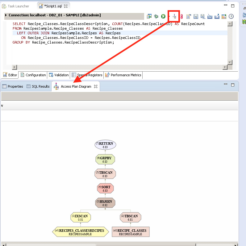
IBM provides some tools to help analyze the explain information, such as the db2exfmt tool to display explain information in formatted output and the db2expln tool to see the access plan information that is available for one or more packages of static SQL, or you can write your own queries against the explain tables. Writing your own queries allows you to customize the output and lets you do comparisons among different queries, or executions of the same query over time, but it does require knowledge of how the data is stored in the explain tables. IBM also provides the capability to generate a diagram of the current access plan through its freely downloadable Data Studio tool (version 3.1 and later). You can download the Data Studio tool at www-03.ibm.com/software/products/en/data-studio. Figure 7.1 illustrates how Data Studio displays the execution plan (using the term “Access Plan Diagram”).
Obtaining an execution plan in Access can be a bit of an adventure. In essence, you turn on a flag telling the database engine to create a text file, SHOWPLAN.OUT, every time it compiles a query, but how you turn that flag on (and where SHOWPLAN.OUT appears) depends on the version of Access you are using.
Turning the flag on involves updating your system registry. For the x86 version of Access 2013 on an x64 operating system, you would use the registry key shown in Listing 7.3.
Listing 7.3 Registry key to turn Show Plan on for Access 2013 x86 on Windows x64
Windows Registry Editor Version 5.00
[HKEY_LOCAL_MACHINE\SOFTWARE\WOW6432Node\Microsoft\Office
\15.0\Access Connectivity Engine\Engines\Debug]
"JETSHOWPLAN"="ON"
Note
The .REG files that can be used to update your registry are included in the Microsoft Access/Chapter 07 folder on the GitHub site (https://github.com/TexanInParis/Effective-SQL). Make sure to read the name of the file carefully to ensure that you use the correct one for your setup.
Note
As mentioned, the exact registry key varies depending on the version of Access being run, and whether you are running a 32-bit or 64-bit version of Access. For example, for Access 2013 on an x86 operating system, the key would be [HKEY_LOCAL_MACHINE\SOFTWARE\Microsoft\Office\15.0\Access Connectivity Engine\Engines\Debug]. For Access 2010 on an x64 operating system, it would be [HKEY_LOCAL_MACHINE\SOFTWARE\WOW6432Node\Microsoft\Office\14.0\Access Connectivity Engine\Engines\Debug]. For Access 2010 on an x86 operating system, it would be [HKEY_LOCAL_MACHINE\SOFTWARE\Microsoft\Office\14.0\Access Connectivity Engine\Engines\Debug].
After you have created that registry entry, you simply run your queries as usual. Every time you run a query, the Access query engine writes the query’s plan to a text file. For Access 2013, SHOWPLAN.OUT is written to your My Documents folder. In some older versions, it was written to the current default folder.
Once you have analyzed all the queries you wish, remember to turn off the flag in your system registry. Again, for the x86 version of Access 2013 on an x64 operating system, you would use the registry key shown in Listing 7.4, but the exact key depends on whichever one you used to turn it on. Unfortunately, there is no built-in tool for graphical viewing of the plan.
Listing 7.4 Registry key to turn Show Plan off for Access 2013 x86 on Windows x64
Windows Registry Editor Version 5.00
[HKEY_LOCAL_MACHINE\SOFTWARE\WOW6432Node\Microsoft\Office
\15.0\Access Connectivity Engine\Engines\Debug]
"JETSHOWPLAN"="OFF"
Note
Former Access MVP Sascha Trowitzsch has written a free Showplan Capturer tool for Access 2010 and earlier, which can be downloaded at www.mosstools.de/index.php?option=com_content&view=article&id=54. This tool allows you to see execution plans without having to update your registry and locate the SHOWPLAN.OUT file.
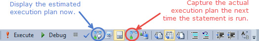
SQL Server provides several ways to fetch an execution plan. A graphical representation is easily accessible in the Management Studio, but because some of the information is visible only when you move the mouse over a particular operation, it is harder to share details with others. Figure 7.2 shows the two different icons on the toolbar, which can be used to produce a graphical execution plan.
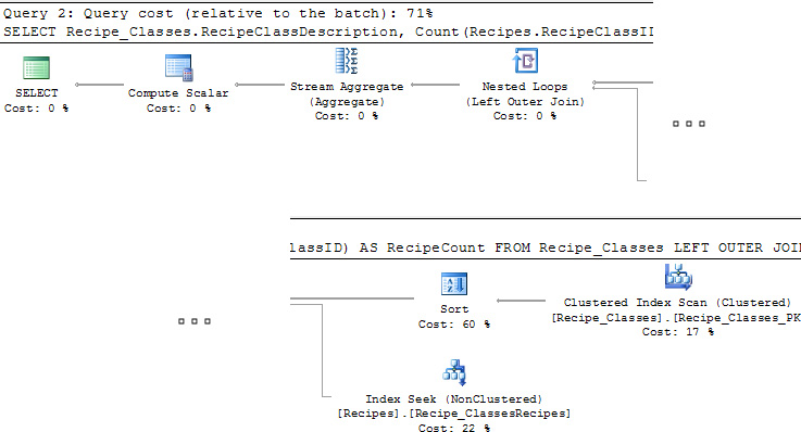
Regardless of which button is used to produce the plan, you will end up with a diagram similar to Figure 7.3 on the next page.
You can compare two queries by placing the SQL for both queries in a new query window, highlighting the SQL for both, and then clicking the Display Estimated Execution Plan button. Management Studio shows you the two estimated plans in the results window. You can obtain an XML version of the execution plan by profiling the execution of an SQL statement. You run the code in Listing 7.5 on the next page to enable it.
Listing 7.5 Enabling execution profiling in SQL Server
SET STATISTICS XML ON;
After you have enabled profiling, every time you execute a statement, you will get an extra result set. For example, if you run a SELECT statement, you will get two result sets: the result of the SELECT statement first, followed by the execution plan in a well-formed XML document.
Note
It is possible to get the output in tabular form, rather than in an XML document, by using SET STATISTICS PROFILE ON (and SET STATISTICS PROFILE OFF). Unfortunately, the tabular execution plan can be hard to read, especially in SQL Server Management Studio, because the information contained in StmtText is too wide to fit on a screen. However, you can copy the information and reformat it to make it more useful. Unlike the graphical plan, you can see all the information at once. We recommend the use of XML instead, especially because Microsoft has indicated that SET STATISTICS PROFILE will be deprecated.
After you have captured all the information you want, you can disable profiling by running the code in Listing 7.6.
Listing 7.6 Disabling execution profiling in SQL Server
SET STATISTICS XML OFF;
Similar to the case for DB2, you can determine the execution plan for any SQL statement in MySQL by prefixing the statement with the word EXPLAIN, as shown in Listing 7.7. (Unlike in DB2, you do not have to do anything first to enable the action.)
Listing 7.7 Creating an execution plan in MySQL
EXPLAIN SELECT CustomerID, SUM(OrderTotal)
FROM Orders
GROUP BY CustomerID;
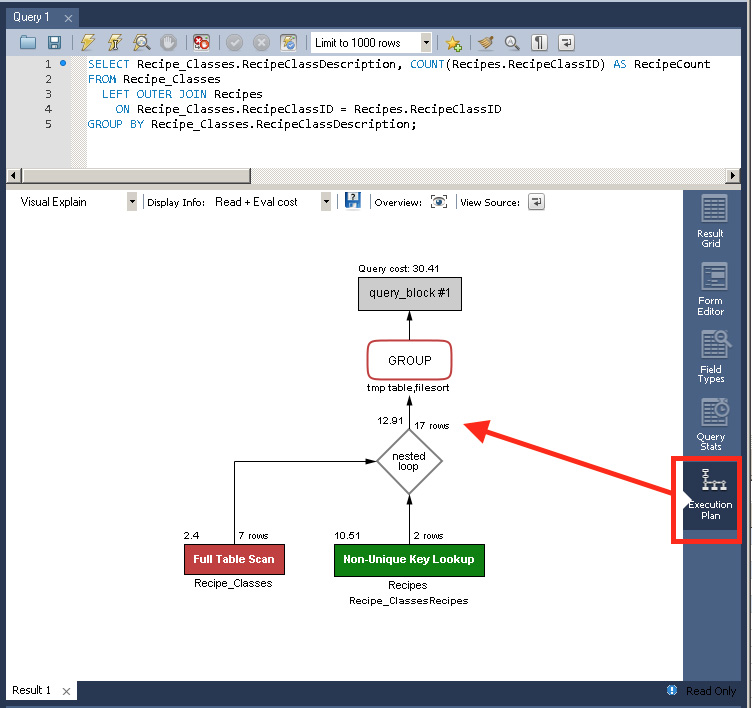
MySQL shows you the plan in tabular form. It is also possible to use the “Visual Explain” feature of the MySQL Workbench 6.2 to provide a visualization of the execution plan, as demonstrated in Figure 7.4.
1. Save the execution plan in the PLAN_TABLE.
2. Format and display the execution plan.
To create the execution plan, you prefix the SQL statement with the keywords EXPLAIN PLAN FOR, as shown in Listing 7.8.
Listing 7.8 Creating an execution plan in Oracle
EXPLAIN PLAN FOR SELECT CustomerID, SUM(OrderTotal)
FROM Orders
GROUP BY CustomerID;
As was the case for DB2, executing the EXPLAIN PLAN FOR command does not actually show the plan. Instead, the system saves the plan into a table named PLAN_TABLE. You should note that the EXPLAIN PLAN FOR command may not necessarily create the same execution plan that the system will use when executing the statement.
Note
The PLAN_TABLE table is automatically available as a global temporary table in release 10g and later. For previous releases, it is necessary to create the table in each schema as needed. You or your database administrator can execute the CREATE TABLE statement from the Oracle database installation ($ORACLE_HOME/rdbms/admin/utlxplan.sql) in any desired schema.
Although it is easy to show execution plans in the Oracle development environment, how they are formatted can vary. A package DBMS_XPLAN was introduced with release 9iR2 that can be used to format and display execution plans from the PLAN_TABLE. For example, the statement in Listing 7.9 shows how to display the most recent execution plan created in the current database session.
Listing 7.9 Displaying the last execution plan explained in the current Oracle database session
SELECT * FROM TABLE(dbms_xplan.display)
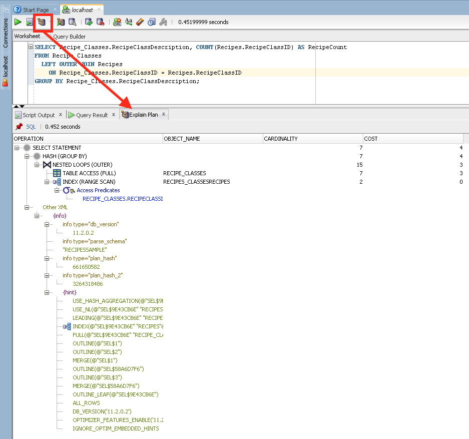
Different tools can display the execution plan information differently. For example, Oracle SQL Developer provides the ability to display the execution plan information in a treelike fashion, as illustrated in Figure 7.5.
Note that some tools are known not to display all of the information, even though it may exist in the PLAN_TABLE.
Note
There are cases when the plan generated by EXPLAIN PLAN FOR and the actual runtime plan do not match, for example, when there are BIND variables with data skew. We advise you to read the Oracle documentation.
You can display execution plans in PostgreSQL by prefixing the SQL statement with the keyword EXPLAIN, as shown in Listing 7.10 on the next page.
Listing 7.10 Creating an execution plan in PostgreSQL
EXPLAIN SELECT CustomerID, SUM(OrderTotal)
FROM Orders
GROUP BY CustomerID;
You can follow the EXPLAIN keyword with one of these options:
 ANALYZE: Carry out the command and show actual run times and other statistics (defaults to
 FALSE).
VERBOSE: Display additional information regarding the plan (defaults to FALSE).
COSTS: Include information on the estimated start-up and total cost of each plan node, as well as the estimated number of rows and the estimated width of each row (defaults to TRUE).
BUFFERS: Include information on buffer usage. May be used only when ANALYZE is also enabled (defaults to FALSE).
TIMING: Include the actual start-up time and time spent in the node in the output. May be used only when ANALYZE is also enabled (defaults to TRUE).
FORMAT: Specify the output format, which can be TEXT, XML, JSON, or YAML (defaults to TEXT).
It is important to note that SQL statements with BIND parameters (e.g., $1, $2, etc.) must be prepared first, as shown in Listing 7.11.
Listing 7.11 Preparing a bound SQL statement in PostgreSQL
SET search_path = SalesOrdersSample;
PREPARE stmt (int) AS
SELECT * FROM Customers AS c
WHERE c.CustomerID = $1;
After the statement has been prepared, its execution can be explained using the statement shown in Listing 7.12.
Listing 7.12 Explaining a prepared SQL statement in PostgreSQL
EXPLAIN EXECUTE stmt(1001);
Note
In PostgreSQL 9.1 version and older, the execution plan was created with the PREPARE call, so it could not consider the actual values provided with the EXECUTE call. Since PostgreSQL 9.2, the execution plan is not created until execution, so it can consider the actual values for the BIND parameters.
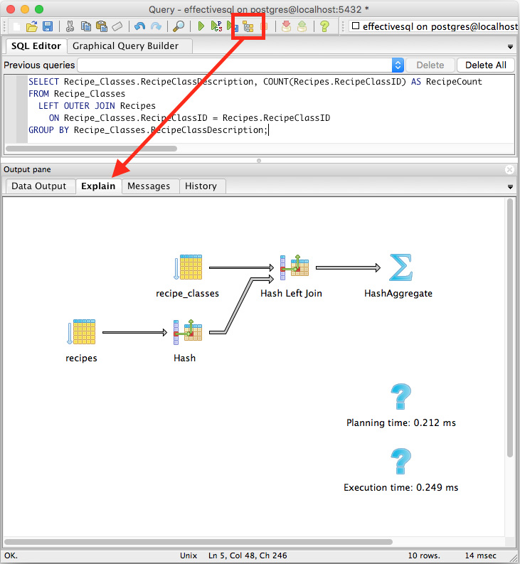
PostgreSQL also provides the pgAdmin tool that can be used to provide a graphical representation of the execution plan via the Explain tab, as Figure 7.6 shows.
 Learn how to obtain execution plans for your DBMS.
Consult the documentation for your DBMS to learn how to interpret the execution plans it produces.
Remember that the information shown in execution plans can change over time.
DB2 requires that system tables be created first. It stores the execution plans in those system tables, as opposed to displaying them. It produces estimated plans.
Access requires that a registry key be installed. It stores the execution plans in an external text file and produces actual plans.
SQL Server requires no initialization to display execution plans. You have the choice of displaying the plans graphically or in tabular form. You also have the choice of producing estimated plans or actual plans.
MySQL requires no initialization to display execution plans. It displays the execution plans to you and produces estimated plans.
Oracle requires no initialization to display execution plans in release 10g and later, although you need to create system tables in each schema of interest for earlier releases. It only stores the execution plans in system tables, as opposed to displaying them. It produces estimated plans.
PostgreSQL requires no initialization to display execution plans. It does, however, require you to prepare SQL statements that have BIND parameters in them. It displays the execution plan for you. For basic SQL statements, it produces estimated plans. For prepared SQL statements, in version 9.1 and older, it produces estimated plans, but since 9.2 it produces actual plans.
Metadata is simply “data about data.” Although you may well have designed an ideal logical database model and worked hard with the DBAs to ensure a proper physical database model (ideally using techniques you have read in this book!), it is often nice to be able to step back and ensure that things were, in fact, implemented consistently with your design. That is where metadata can help.
ISO/IEC 9075-11:2011 Part 11: Information and Definition Schemas (SQL/Schemata) is an often-overlooked part of the official SQL Standards. This standard defines the INFORMATION_SCHEMA, which is intended to make SQL databases and objects self-describing.
When a physical data model is implemented in a compliant DBMS, not only are each of the objects such as tables, columns, and views created in the database, but also your system stores information about each of those objects in system tables. A set of read-only views exists on those system tables, and those views can provide information about all the tables, views, columns, procedures, constraints, and everything else necessary to re-create the structure of a database.
Note
Although INFORMATION_SCHEMA is an official standard of the SQL language, the standard is not always followed. While IBM DB2, Microsoft SQL Server, MySQL, and PostgreSQL all provide INFORMATION_SCHEMA views, Microsoft Access and Oracle do not at present (although Oracle does provide internal metadata that can serve the same needs).
There are a variety of third-party products that can provide you with information about your database. Most of them do so by retrieving information from the INFORMATION_SCHEMA views. You do not need a third-party tool, though, to be able to get useful information from those views.
Let’s assume you have been given access to a new database, and you want to find out details about it.
You can query the INFORMATION_SCHEMA.TABLES view to get a list of the tables and views that exist in the database, as shown in Listing 7.13, the results of which are shown in Table 7.1.
Listing 7.13 Get a list of tables and views
SELECT t.TABLE_NAME, t.TABLE_TYPE
FROM INFORMATION_SCHEMA.TABLES AS t
WHERE t.TABLE_TYPE IN ('BASE TABLE', 'VIEW');
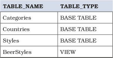
Table 7.1 List of tables and views from Listing 7.13
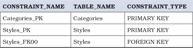
You can query the INFORMATION_SCHEMA TABLE_CONSTRAINTS view to get a list of what constraints have been created on those tables, as shown in Listing 7.14, with results shown in Table 7.2 on the next page.
Listing 7.14 Get a list of constraints
SELECT tc.CONSTRAINT_NAME, tc.TABLE_NAME, tc.CONSTRAINT_TYPE
FROM INFORMATION_SCHEMA.TABLE_CONSTRAINTS AS tc;
Table 7.2 List of constraints from Listing 7.14
Yes, there are definitely other ways to obtain that same information. However, the fact that the information is available in views allows you to determine more information. For example, since you know all of the tables in your database and you know all of the table constraints that have been defined, you can easily determine which tables in your database do not have a primary key, as shown in Listing 7.15, with results shown in Table 7.3.
Listing 7.15 Get a list of tables without a primary key
SELECT t.TABLE_NAME
FROM (
SELECT TABLE_NAME
FROM INFORMATION_SCHEMA.TABLES
WHERE TABLE_TYPE = 'BASE TABLE'
) AS t
LEFT JOIN (
SELECT TABLE_NAME, CONSTRAINT_NAME, CONSTRAINT_TYPE
FROM INFORMATION_SCHEMA.TABLE_CONSTRAINTS
WHERE CONSTRAINT_TYPE = 'PRIMARY KEY'
) AS tc
ON t.TABLE_NAME = tc.TABLE_NAME
WHERE tc.TABLE_NAME IS NULL;
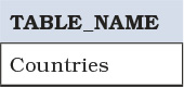
Table 7.3 List of tables without a primary key from Listing 7.15
Should you be considering making a change to a particular column, you can use the INFORMATION_SCHEMA.VIEW_COLUMN_USAGE view to see which table columns are being used in any view, as shown in Listing 7.16.
Listing 7.16 Get a list of all tables and columns used in any view
SELECT vcu.VIEW_NAME, vcu.TABLE_NAME, vcu.COLUMN_NAME
FROM INFORMATION_SCHEMA.VIEW_COLUMN_USAGE AS vcu;
As shown in Table 7.4, it does not matter whether or not you have used an alias for any of the column names, or even if the column appears only in the WHERE or ON clause of the view. This information allows you to see quickly whether your possible change might have any impacts.
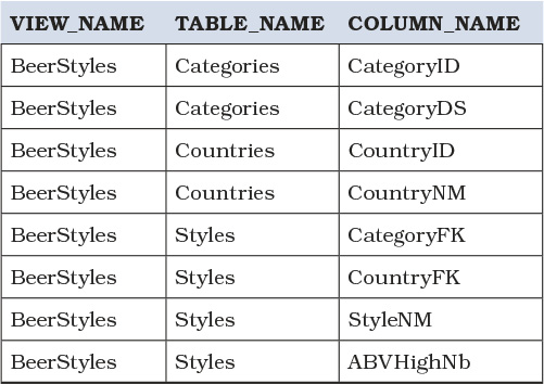
Table 7.4 List of all tables and columns used in any view from Listing 7.16
Listing 7.17 shows the SQL used to create the BeerStyles view. You can see that INFORMATION_SCHEMA.VIEW_COLUMN_USAGE reports on all columns used, whether they are in the SELECT clause, the ON clause, or anywhere else in the CREATE VIEW statement.
Listing 7.17 CREATE VIEW statement for the view documented in Table 7.4
CREATE VIEW BeerStyles AS
SELECT Cat.CategoryDS AS Category, Cou.CountryNM AS Country,
Sty.StyleNM AS Style, Sty.ABVHighNb AS MaxABV
FROM Styles AS Sty
INNER JOIN Categories AS Cat
ON Sty.CategoryFK = Cat.CategoryID
INNER JOIN Countries AS Cou
ON Sty.CountryFK = Cou.CountryID;
A major advantage of using INFORMATION_SCHEMA rather than DBMS-specific metadata tables is that because INFORMATION_SCHEMA is an SQL standard, any queries you write should be portable from DBMS to DBMS, as well as from release to release of any specific DBMS.
That being said, you should probably be aware that there can be issues with using INFORMATION_SCHEMA. For one thing, despite being a standard, INFORMATION_SCHEMA is not actually implemented consistently from DBMS to DBMS. The INFORMATION_SCHEMA.VIEW_COLUMN_USAGE view that we showed in Listing 7.16 does not exist in MySQL, but it does in SQL Server and PostgreSQL.
Additionally, because INFORMATION_SCHEMA is a standard, it is designed to document only features that exist in the standards. And even when the feature is permitted, it is still possible that INFORMATION_SCHEMA may not be capable of documenting it. An example of this is creating FOREIGN KEY constraints that reference unique indexes (as opposed to primary key indexes). Usually you would document FOREIGN KEY constraints by joining the REFERENTIAL_CONSTRAINTS, TABLE_CONSTRAINTS, and CONSTRAINT_COLUMN_USAGE views in INFORMATION_SCHEMA, but because a unique index is not a constraint, there is no data in TABLE_CONSTRAINTS (or in any other constraint-related view), and you cannot determine which columns are used in the “constraint.”
Fortunately, all DBMSs have other metadata sources available, and you can use them to determine information as well. The downside, of course, is that what you have learned that works in one DBMS may not work in another DBMS.
For instance, you could retrieve the same information retrieved in Listing 7.13 in SQL Server using the SQL statement in Listing 7.18.
Listing 7.18 Get a list of tables and views using SQL Server system tables
SELECT name, type_desc
FROM sys.objects
WHERE type_desc IN ('USER_TABLE', 'VIEW');
Alternatively you can use the SQL statement in Listing 7.19 to get the same information in SQL Server as provided by Listing 7.18.
Listing 7.19 Get a list of tables and views using different SQL Server system tables
SELECT name, type_desc
FROM sys.tables
UNION
SELECT name, type_desc
FROM sys.views;
It is perhaps telling that even Microsoft seems not to trust INFORMATION_SCHEMA: there are many places on MSDN, such as https://msdn.microsoft.com/en-us/library/ms186224.aspx, where they state:
**Important** Do not use INFORMATION_SCHEMA views to determine the schema of an object. The only reliable way to find the schema of an object is to query the sys.objects catalog view. INFORMATION_SCHEMA views could be incomplete because they are not updated for all new features.
Note
Many DBMSs offer alternative means of getting to their metadata. For example, DB2 has a db2look command, MySQL has a SHOW command, Oracle has a DESCRIBE command, and PostgreSQL’s command-line interface psql has a \d command, all of which can be used to query data. Consult your documentation to determine what options you have. However, those commands do not permit you to query the metadata using SQL as shown in the previous listings, so also check the documentation for system tables or schema if you need to collect information from several objects at once or within the context of an SQL query.
Use the SQL standard INFORMATION_SCHEMA views whenever possible.
Remember that INFORMATION_SCHEMA is not the same across DBMSs.
Learn any nonstandard command your DBMS may have to display metadata.
Accept that INFORMATION_SCHEMA does not contain 100% of the necessary metadata, and learn the system tables associated with your DBMS.
Because this is a book about SQL, and not about any particular vendor’s product, it is difficult to be very specific, because the execution plan is dependent on the physical implementation. Each vendor has a different implementation and uses different terminology for the same concepts. However, it is an essential skill for anyone working with an SQL database to understand how to read and understand what an execution plan means in order to be able to optimize SQL queries or make any needed schema changes, especially on indices or model design. Thus we will focus on some general principles that you might find useful when reading an execution plan for your SQL database, regardless of which vendor’s product you use. This item is intended to be supplemented with additional readings in the vendor’s documentation on reading and interpreting the execution plan.
We also want to remind readers that the goal of SQL is to free developers from the menial task of describing the physical steps to retrieve the data, especially in an efficient manner. It is meant to be declarative, describing what data we want to get back and leaving it up to the optimizer to figure out the best way to get it. When we discuss execution plans, and therefore the physical implementation, we are breaking the abstraction that SQL offers.
A common mistake that even computer-literate people make is to assume that because a task is done by a computer, it is magically different from the way it would be done by a person. It just ain’t so. Yes, a computer might execute and complete a task much faster and more accurately, but the physical steps it must take are no different from those of an actual person doing the same task. Consequently, when you read an execution plan, you get an outline of physical steps the database engine performs to satisfy a query. You can then ask yourself, if you were doing it yourself, whether you would get the best result.
Consider a card catalog in a library. If you wanted to locate a book named Effective SQL, you would go to the catalog and locate the drawer that contains cards for books starting with the letter E (maybe it will actually be labeled D–G). You would then open the drawer and flip through the index cards until you find the card you are looking for. The card says the book is located at 601.389, so you must then locate the section somewhere within the library that houses the 600 class. Arriving there, you have to find the bookshelves holding 600–610. After you have located the correct bookshelves, you have to scan the sections until you get to 601, and then scan the shelves until you find the 601.3XX books before pinpointing the book with 601.389.
In an electronic database system, it is no different. The database engine needs to first access its index on data, locate the index page(s) that contains the letter E, then look within the page to get the pointer back to the data page that contains the sought data. It will jump to the address of the data page and read the data within that page(s). Ergo, an index in a database is just like the catalog in a library. Data pages are just like bookshelves, and the rows are like the books themselves. The drawers in the catalog and the bookshelves represent the B-tree structure for both index and data pages.
We made you walk through this to emphasize the point that when you read the execution plan, you can easily apply the physical action, as though you were doing the same thing with papers, folders, books and index cards, labels, and the classification system. Let’s do one more thought experiment. Now that you have found the Effective SQL book that John Viescas coauthored, you want to find out what other books he has written. You cannot go back to the catalog because that catalog sorts the index cards by book title, not by author. Without a catalog available, the only way to answer the question is to painstakingly go through every bookshelf, each of the shelves, and each book to see what other books John has authored. If you found that such questions were commonly asked, it would be more expedient to build a new catalog, sorted by author, and put it beside the original catalog. Now it is easy to find all books that John has authored or coauthored just by looking in the new catalog—no more trips to the bookshelves. But what if the question changes and is now “How many pages are there in each book that John wrote?” Well, that extra piece of information is not in the index cards. So it is back to the bookshelves to find out the page counts in each book.
This illustrates the next key point: the index system you set up depends heavily on what kind of queries you will typically use against your database. You needed two catalogs to support different types of queries. Even so, there were still some gaps. Is the correct answer to add page counts to the index cards in one of the catalogs? Maybe, maybe not. It depends more on whether it is essential that you get the information quickly.
It is also possible to have queries where you never need to actually go to the bookshelves. For example, if you wanted a list of all authors with whom John has written books, you could look up all books that John has co-written, but the catalog does not list the other authors for those books. But you can then look in the book titles catalog, look up the title that you got from the author catalog, and thus get the list of coauthors. You were able to do all this standing at the catalogs without going to the bookshelves at all. Thus, this is the fastest way to retrieve data.
The preceding thought experiments should make it clear that when you read the execution plan, you can act out the physical actions in your mind. So, if you saw an execution plan that scans a table, and you know you have an index that exists but apparently is not used in the plan (as though you had walked past the catalog and gone directly to the bookshelves), you can tell something is amiss and start your analysis.
Note
The examples provided in the rest of the items are heavily dependent on the data stored in the database, the existing index structure, and other things. Therefore, it might not always be possible to reproduce the exact same execution plan. The examples also use the Microsoft SQL Server execution plan, as it provides a graphical view. Other vendors might yield similar plans but use different terms.
With the mental scaffolding set up, let’s look at some examples, starting with Listing 7.20.
Listing 7.20 Query to find customers’ cities based on an area code
SELECT CustCity
FROM Customers
WHERE CustAreaCode = 530;
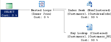
In a large enough table, we might get the plan illustrated in Figure 7.7.
To translate this into physical actions, think of it as going to a catalog containing the CustAreaCode and location code on the index cards. For each index card found, we then go to the bookshelves, locate the record to read the CustCity value, then return to the catalog to read the next index. That is what is meant when you see a “Key Lookup” operation. An “Index Seek” operation represents looking through the catalog, whereas “Key Lookup” means you are going to the bookshelves to get the additional information that is not contained on the index card.
For a table with few records, it is not that bad. But if it turns out that we found many index cards and shuttled between the bookshelves and the catalog, that is a lot of wasted time. Let’s say there are several possible matches. If the query is commonly asked, it makes sense to update the index to include the CustCity. One way to do this is with the SQL statement in Listing 7.21.
Listing 7.21 Improved index definition
CREATE INDEX IX_Customers_CustArea
ON Customers (CustAreaCode, CustCity);
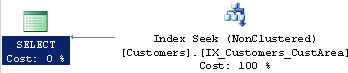
This changes the execution plan to what is shown in Figure 7.8 for the same query.
So we are back to standing at the new catalog and reading through the index cards without going to the bookshelves at all. That is much more efficient even though we now have one more catalog in the library.
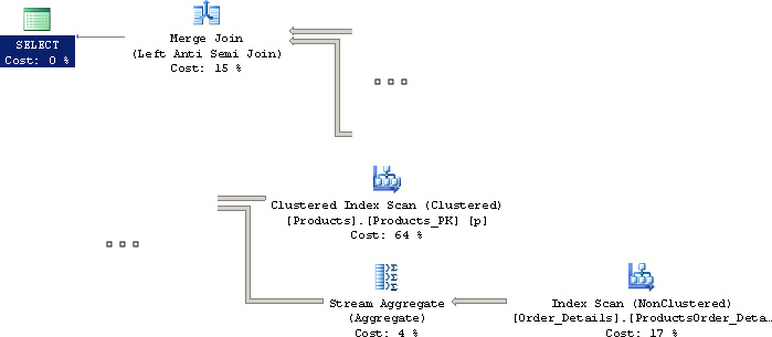
It is also important to note that sometimes the physical steps described by a generated execution plan can be quite different from the logical steps described by the SQL query itself. Consider the query that does an EXISTS correlated subquery in Listing 7.22.
Listing 7.22 Query to find customers who have not placed any orders
SELECT p.*
FROM Products AS p
WHERE NOT EXISTS (
SELECT NULL
FROM Order_Details AS d
WHERE p.ProductNumber = d.ProductNumber
);
At a glance, it looks as if the engine must query the subquery for each row in the Products table because we are using a correlated subquery. Let’s consider the execution plan in Figure 7.9.
To translate the execution plan into physical actions: with “Clustered Index Scan” on Products, we first grab a stack of index cards from one catalog that detail the products we have on hand. With “Index Scan” on Order_Details, we grab another stack of index cards from the catalog containing orders. For “Stream Aggregate,” we group all index cards containing the same ProductNumber. Then for “Merge Join,” we sort through both stacks, taking out a product index card only if we do not have a matching card from the Order_Details stack. That gives us the answer. Take note that the merge join is a “left anti-semi-join”; this is a relational operation that has no direct representation in the SQL language. Conceptually, a semi-join is like a join except that you select a row that matches only once rather than for all matching rows. Therefore, an anti-semi-join selects distinct rows that do not match the other side.
So in this specific example, the engine was smart enough to see a better way of doing things and rearranged the execution plan accordingly. However, it bears emphasizing that the engine itself is constrained by the user asking the queries. If we send it poorly written queries, it has no choice but to generate poor execution plans.
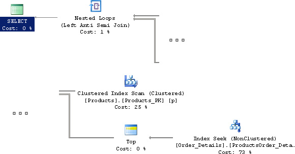
When you read your execution plans, you check whether the engine is making sane choices as to how it should collect the data and doing it in the most efficient manner. Because the execution plan is a sequence of physical actions, it can vary drastically even for the same query if the data volume and distribution change. For example, using the same query from Listing 7.22 on a smaller set of data, we might get the plan shown in Figure 7.10.
What is not apparent is that the “Index Seek” on the Order_Details table has a predicate to take a value from the “Clustered Index Scan” on the Products table. The “Top” operation then restricts the output to only one row and matches to the records from the Products table. This is similar to the key lookup we saw earlier. Because the data set was small enough, the database engine decided it was good enough to do a key lookup instead of taking a stack, because that is less setup to do.
That then brings us to the problem of “elephant and mouse.” By now you should realize that there are many possible sequences of physical actions to get the same results. However, which sequence is more effective depends on the data distribution. So it is possible to have a parameterized query that performs great for a particular value but is awful with a different value. This is a particular problem for any engines that cache an execution plan for a parameterized query (which might be a stored procedure, for instance). Consider the simple parameterized query in Listing 7.23.
Listing 7.23 Query to find order details for a particular product
SELECT o.OrderNumber, o.CustomerID
FROM Orders AS o
WHERE EmployeeID = ?;
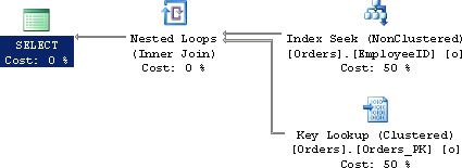
Suppose we pass in EmployeeID = 751. That employee made 99 orders out of 160,944 rows in the Orders table. Because there are comparatively few records, the engine might create a plan like the one in Figure 7.11.
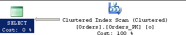
Contrast that with the plan where we pass in EmployeeID = 708 who has worked on 5,414 orders in Figure 7.12.
Because the engine saw that there were so many records scattered, it decided it was just as fast to wade through all the data. This is obviously suboptimal, and we can improve it by adding an index specifically for this query as shown in Listing 7.24.
Listing 7.24 Index to cover the query in Listing 7.23
CREATE INDEX IX_Orders_EmployeeID_Included
ON Orders (EmployeeID)
INCLUDE (OrderNumber, CustomerID);
Because the index covers both queries, this improves the plan for both “mouse” and “elephant” significantly, as shown in Figure 7.13.
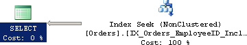
Figure 7.13 Improved execution plan for the query in Listing 7.23
However, this might not be possible in all cases. In a complicated query, it might not make sense to create an index that would be usable in only one query. You want to have an index that is useful in several queries. For that reason, you might elect to modify the columns indexed or included in an index and even exclude some.
In those situations, the “mouse and elephant” problem can still appear for parameterized queries. In those situations, it is likely best to recompile the queries, because compilation of a query is usually a fraction of the total execution time. You should investigate what options you have available for your database product for forcing recompilation where it is applicable. With some database engines such as Oracle, peeking into the parameters prior to executing the cached plan is supported, which helps alleviate this particular problem.
Whenever you read an execution plan, translate it into physical actions, analyze whether you have indices that are not being used, and determine why they are not being used.
Analyze the individual steps and consider whether they are effective. Note that efficiency is influenced by the data distribution. Consequently, there are no “bad” operations. Rather, analyze whether the operation used is appropriate for the query being used.
Do not fixate on one query and add indices to get a good execution plan. You must consider the overall usage of the database to ensure that indices serve as many queries as possible.
Watch out for a “mouse and elephant” situation, where the data distribution is unequal and thus requires different optimizations for an identical query. That is especially problematic when execution plans are cached and reused (typically the case with stored procedures or client-side prepared statements).