Chapter 2. How Automated Machine Learning Works

In the previous chapter, we established the need to automate the process of building machine learning models. In this chapter, we explain what Automated Machine Learning is, the different techniques involved in this process, and how they all come together. We will also give a quick overview of automated ML on Microsoft Azure Machine Learning.

What Is Automated Machine Learning?

In Chapter 1, we discussed how coming up with a good machine learning model can be time-consuming and tedious, given all the possible combinations to explore. Automated Machine Learning is a recent development in machine learning focused on making that entire process easy, with the goal of bringing efficiency to data scientists as well as enabling non–data scientists to build models.

Let’s go through the stages of the machine learning process and see how Automated Machine Learning can help at each stage.

Understanding Data

As briefly discussed in the previous chapter, real-world data is not clean and requires a lot of effort to get to a usable state. Understanding input data is a crucial step toward formulating the machine learning problem.

Automated Machine Learning can help here by analyzing the data and automatically detecting the data type of each column. Column types could be Boolean, numeric (discrete or continuous), or text. Automatically detecting these column types helps with subsequent stages like feature engineering.

In many cases, Automated Machine Learning can also provide insight into the semantics or intent of each column. It can detect a wide spectrum of situations, including the following:

• Detecting the target/label column

• Detecting whether a text column is a categorical-text feature or free-text feature

• Detecting columns that are zip codes, temperatures, geo coordinates, and so on

Before we go ahead, let’s discuss how the model training process works in relationship to input data. Should we train using all of the data available? The answer is no.

Training the model on the full input data can lead to overfitting. Overfitting means that the model we trained is fit too closely to the input dataset and mimics the input dataset. This usually happens when the model is too complex (i.e., too many features/variables compared to the number of observations). This model will be very accurate on the input data but will probably perform badly on untrained or new data.

In contrast, when a model is underfit, it means that the model does not fit the input data and therefore misses the trends in the data. It also means the model cannot be generalized to new data. This is usually the result of a very simple model (not enough input variables/features). Adding more input variables/features helps overcome underfitting.

Figure 2-1 shows overfitting and underfitting for a binary classification problem.

Figure 2-1. Overfitting and underfitting

To overcome the overfitting problem, we usually split input data into two subsets: training data and testing data (and sometimes further, into three subsets: train, validate, and test). The model is then fit on the training data to make predictions on the test data. The training set contains a known output, and the model learns on this so that it can generalize to other data later. We use the test set to test the accuracy of our model’s predictions.

But, how do we know if the train/test split is good? What if one subset of our data is skewed compared to the other? This will result in overfitting, even though we’re trying to avoid that. This is where cross-validation comes in.

Cross-validation is similar to the train/test split, but it’s applied to more subsets. Data is split into k subsets, and the model is trained on k – 1 of those subsets. The last subset is held for testing. This is done for each of the subsets. This is called k-fold cross-validation. Finally, the scores from all the k-folds are averaged to produce the final score. Figure 2-2 shows this.

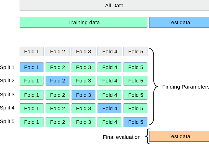
Figure 2-2. k-fold cross-validation (source: ttps://oreil.ly/k-ixI)

Detecting Tasks

Data scientists map real-world scenarios to machine learning tasks. Figure 2-3 shows some examples of types of machine learning tasks.

Figure 2-3. Machine learning tasks

Automated Machine Learning can automatically determine the machine learning task, given the input data. This is more relevant in supervised machine learning, in which target/label columns can be used to predict the machine learning task. Table 2-1 lists generic machine learning tasks.

Table 2-1. Machine learning task detection

Target/Label column	Machine learning task	Example scenarios
Boolean	Binary classification	* Classifying sentiment of Twitter comments as either positive or negative * Indicating that email is spam or not
Discrete numerical/categorical	Multiclass classification	* Determining the breed of a dog as Havanese, Golden Retriever, Beagle, etc. * Categorizing hotel reviews by location, price, cleanliness, etc.
Continuous numerical	Regression	* Predicting house prices based on house attributes such as number of bedrooms, location, or size * Predicting future stock prices based on historical data and current market trends

In addition to these generic tasks, there are specific variations based on input data. Forecasting is one such task type that is popular, given its relevance to many business problems like revenue forecasting, inventory management, predictive maintenance, and so on. If input data is time-series, determined by availability of a DateTime column, it is most likely a forecasting task.

Choosing Evaluation Metrics

Choosing a metric to evaluate your machine learning algorithm is fundamentally driven by the business outcome. This is an important step because it tells you how the performance of your algorithm is measured and compared. Different tasks have different sets of evaluation metrics to choose from, and the choice depends on multiple factors. Figure 2-4 shows possible options for evaluating algorithms used in various machine learning tasks.

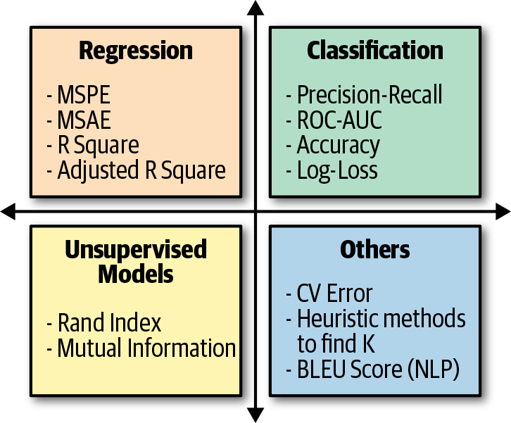
Figure 2-4. Machine learning evaluation metrics

Automated Machine Learning can automate the process of selecting the right evaluation metric for a given input dataset and machine learning task. For instance, scenarios like fraud detection (which is a classification task) inherently have imbalanced data in that a very small percentage of data would be fraudulent. In this case, area under curve (AUC) is a much better evaluation metric than accuracy. Automatically detecting class imbalance in the data can help automatically choose AUC as an evaluation metric for this classification task.

Feature Engineering

As discussed in Chapter 1, feature engineering is the process of getting to the appropriate set of features from input data with the goal of producing a good machine learning model. Automated feature engineering involves four key steps, which we discuss in the subsections that follow.

Detect issues with input data and automatically flag them

Examples of this include the following:

• Detecting missing values and automatically imputing them with the most relevant technique; for example, numeric columns with mean, categorical columns with mode (most frequently occurring), and so on.

• Detecting class imbalance and automatically fixing it by applying techniques like the Synthetic Minority Oversampling Technique (SMOTE).

Drop columns that are not useful as features

Here are some examples:

No variance columns

These are columns with the same value across all rows, which are easy to detect via automation.

High cardinality columns

These are columns with different values across rows; for example, hashes, IDs, or globally unique identifiers (GUIDs). Cardinality is determined by percentage of unique values in the column.

Generate features

There are multiple techniques for generating new features from existing features. Some examples follow:

Encodings and transformations

Most machine learning algorithms require numerical input and output variables. Real-world datasets are full of text and categorical data. Data scientists convert them into numerical data by using encodings and transformations.

One-hot encoding is a popular technique to convert categorical data to integer data. You can easily automate this process. Figure 2-5 shows an example of one-hot encoding.

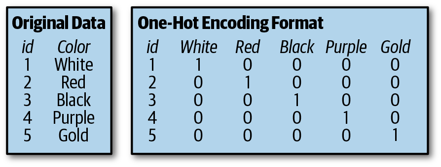
Figure 2-5. One-hot encoding

Transformations are applied to input columns to generate interesting features. Some examples include generating “Year,” “Month,” “Day,” “Day of week,” “Day of year,” “Quarter,” “Week of the year,” “Hour,” “Minute,” and “Second” for a given DateTime column. This is effective for time-series-related problems.

Other examples might generate term frequency based on unigrams, bi-grams, and tri-character-grams, and generating word embeddings for text columns.

Aggregations

Another popular technique in feature generation involves generating aggregations over multiple data records. Aggregations could be based on specific entities in the dataset (e.g., average product sales/revenue per store) or based on time (e.g., number of page views to a website in the past 7 days, 30 days, 180 days, etc.). Features generated through time-based aggregations are quite useful for time-series forecasting problems.

Select the most impactful features

Feature selection is an important step in the process because it helps to prioritize the appropriate set of input features. This becomes even more important when the number of input features is very large.

Why do we need to prioritize the proper set of input features? Why not use all the features? Here are the top benefits of feature selection:

• Faster training

• Simpler model, easier to interpret

• Reduces overfitting

• Improved model accuracy

Let’s go through some different feature selection techniques. Keep in mind that you can automate all of these techniques:

Filters

According to this technique, the selection of features is independent of any machine learning algorithms. Features are selected based on their correlation with the outcome variable, as measured by statistical tests. Because the selection process is agnostic of the model, this method might not select the most useful features but is robust against overfitting. As shown in Figure 2-6, selecting the best subset of features happens before model training.

Wrappers

According to this technique, a subset of features is used to train a model. Based on the performance of the model, we decide to add or remove features from the subset and train the model again with the updated subset. This process continues until the model’s performance is satisfactory. However, this technique can be computationally expensive due to multiple back-and-forth iterations. Because the selection process is tied to the model, it tends to produce more accurate results than filter methods but is more prone to overfitting. Figure 2-6 demonstrates wrapper methods.

Embedded methods

Embedded methods combine the qualities of filter and wrapper methods. Implemented by algorithms that have their own built-in feature selection methods, embedded methods are like wrappers but are less computationally expensive because there are no back-and-forth iterations. This technique is also less prone to overfitting. Figure 2-6 demonstrates embedded methods.

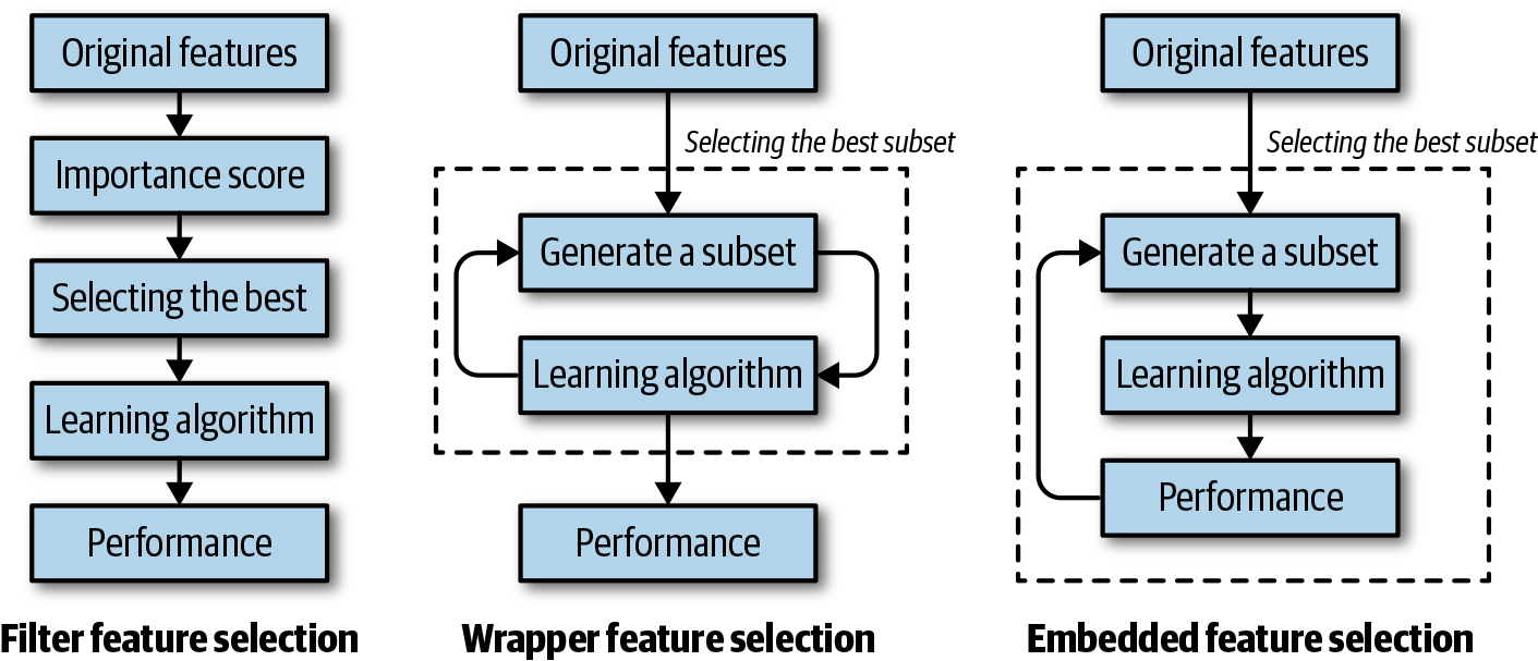
Figure 2-6. Feature selection

Selecting a Model

As discussed in the previous chapter, a machine learning model is represented by a combination of an algorithm and associated hyperparameter values. Automated Machine Learning systems follow different approaches for model selection. In this section, we discuss two categories of approaches: brute-force approaches and smarter approaches.

Brute-force approaches

This is the naïve approach of trying out all possible combinations of algorithms and hyperparameter values to find the one that produces the best model as measured by the evaluation metric. This is typically achieved by picking algorithms at random and applying grid search to figure out the right set of hyperparameters. One major drawback of grid search is that dimensionality suffers when the number of hyperparameters grows exponentially. With as few as four parameters, this problem can become impracticable because the number of evaluations required for this approach increases exponentially with each additional parameter, due to the curse of dimensionality.

Random search is a technique by which random combinations of the hyperparameters are used to find the best solution. In this search pattern, random combinations of parameters are considered in every iteration. Because random values are selected at each iteration, it is highly likely that the whole space has been covered due to randomness; hence the chances of finding the best model are comparatively higher than grid search. It takes a huge amount of time to cover every aspect of the combination during grid search. Random search works best if all hyperparameters are not equally important.

Figure 2-7 shows how grid search and random search work. In this example, nine sets of parameter combinations are being tried. Notice how random search manages to reach much better model performance, as shown by the dots on the “hills” at top. The topmost point on the “hill” represents the best parameter combination.

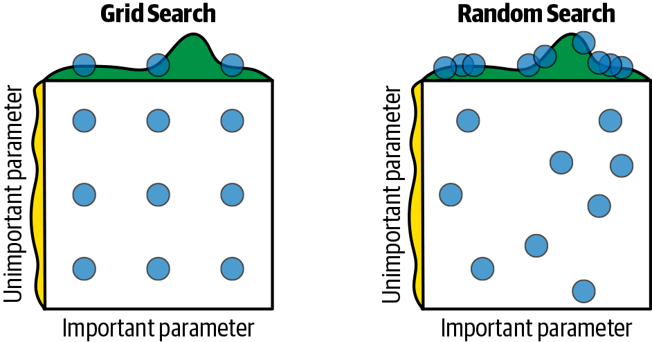
Figure 2-7. Grid search versus random search

Smarter approaches

For real-world problems, the search space is very large, and brute-force approaches will not be effective. This has led to the emergence of smarter selection and optimizations approaches, mostly powered by advanced statistics and machine learning techniques. Some of these approaches include Bayesian optimization, multiarmed bandit, and meta-learning. Here, we describe some of these at a high level (details require digging deeper and are beyond the scope of this book):

Bayesian optimization

This method uses approximation to guess an unknown function with some prior knowledge. The goal here is to train the model based on available observations. The trained model will map to a function, which we don’t know. Our task is to find the hyperparameters that maximize the learning function.

Bayesian optimization can help you find the best model among many, speeding up the model selection process by reducing the computation task and not requiring help from a human to guess the values. This optimization technique is based on randomness and probability distributions. Figure 2-8 provides a visual description of how it works.

Figure 2-8. Bayesian optimization

The dotted line is our True Objective function curve. Unfortunately, we don’t know this function and its equation. We are trying to approximate it by using a Gaussian process. Throughout our sample space, we draw an intuitive curve (the solid line) that fits with our observed samples (the solid dots). t represents different time points when we have a new observation sample. The shaded region is the Confidence region, where the point could exist. From the preceding prior knowledge, we can determine that second point as the maximum observed value. The next maximum point should be above it or equal. If we draw a horizontal line through the second point, the next maximum point should fall above this line. From the intersecting points of this line and the Confidence region, we can discard the curve samples below the line to find the maximum. In so doing, we have narrowed down our area of investigation. This same process continues with the next sampled points.

Multiarmed bandit

A multiarmed bandit is a problem in which a limited set of resources must be allocated between competing choices in a way that maximizes their expected gain when each choice’s properties are only partially known at the time of allocation and might become better understood as time passes or by allocating resources to the choice.

This is a classic reinforcement learning problem covering the exploration–exploitation trade-off dilemma, modeling an agent that simultaneously attempts to acquire new knowledge (called exploration) and optimize its decisions based on existing knowledge (called exploitation). As shown in Figure 2-9, the agent attempts to balance these competing tasks to maximize its total value over the period considered.

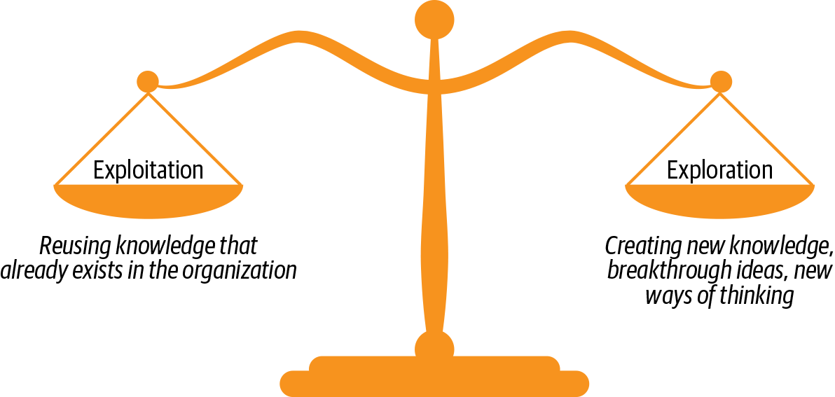
Figure 2-9. Explore versus exploit

Meta-learning

This “learning to learn.” Think of this as applying machine learning to build machine learning models; hence, the term “meta” in the name. The goal of meta-learning is to train a model on a variety of learning tasks, such that it can solve new learning tasks with only a small number of training samples. Not only does this dramatically speed up and improve the design of machine learning pipelines, but also allows us to replace a fixed set of manually chosen models with novel approaches learned in a data-driven way.

With neural networks gaining popularity, meta-learning approaches have been applied to automatically design optimal neural network architectures. Known as neural architecture search (NAS), this is a popular area of research. NAS has been used to design networks that are on par with or outperform hand-designed architectures. Methods for NAS can be categorized according to the search space, search strategy, and performance estimation strategy used.

The search space defines the type(s) of neural networks that can be designed and optimized. The search strategy defines the approach used to explore the search space. The performance estimation strategy evaluates the performance of a possible neural network from its design (without constructing and training it).

Monitoring and Retraining

So far, we have covered the stages leading up to building a good model and how Automated Machine Learning can help with each of those stages. The last and final stage in the machine learning workflow is monitoring and retraining your model.

Model performance during training can be very different from its performance after deployment on real data. Thus, it is important to continuously measure model performance even after deployment. Poor model performance is typically caused by change in characteristics of input data over time, which is known as data drift. Techniques exist to automatically monitor data drift and model performance over time.

As soon as poor model performance is detected, corrective actions can be taken to minimize the damage. Corrective actions could include the following:

• Immediately take the model offline (and disable the corresponding user experience)

• Retrain the model with the latest data and deploy the retrained model

This stage is particularly critical for companies that have production dependency on machine learning models. Hence, a good Automated Machine Learning solution should have support for monitoring and training.

Bringing It All Together

Automated Machine Learning empowers users (with or without machine learning expertise) to identify an end-to-end machine learning pipeline for any problem, achieving higher accuracy while spending far less of their time. And it enables a significantly larger number of experiments to be run, resulting in faster iteration toward production-ready intelligent experiences. Given input data, it can automate the process of feature engineering, model selection, and hyperparameter tuning, as shown in Figure 2-10.

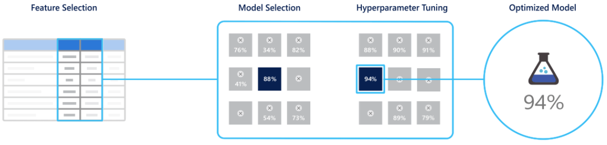
Figure 2-10. Automated Machine Learning

Automated ML

Automated ML is a capability available within the Microsoft Azure Machine Learning service. This section provides an overview of how automated ML works, whereas subsequent chapters will go into more details on how to use automated ML for your scenarios.

How Automated ML Works

Automated ML is based on a breakthrough from the Microsoft Research division. The approach combines ideas from collaborative filtering and Bayesian optimization to search an enormous space of possible machine learning pipelines intelligently and efficiently. It’s essentially a recommender system for machine learning pipelines. Similar to how streaming services recommend movies for users, automated ML recommends machine learning pipelines for datasets. Figures 2-11 and 2-12 demonstrate this analogy.

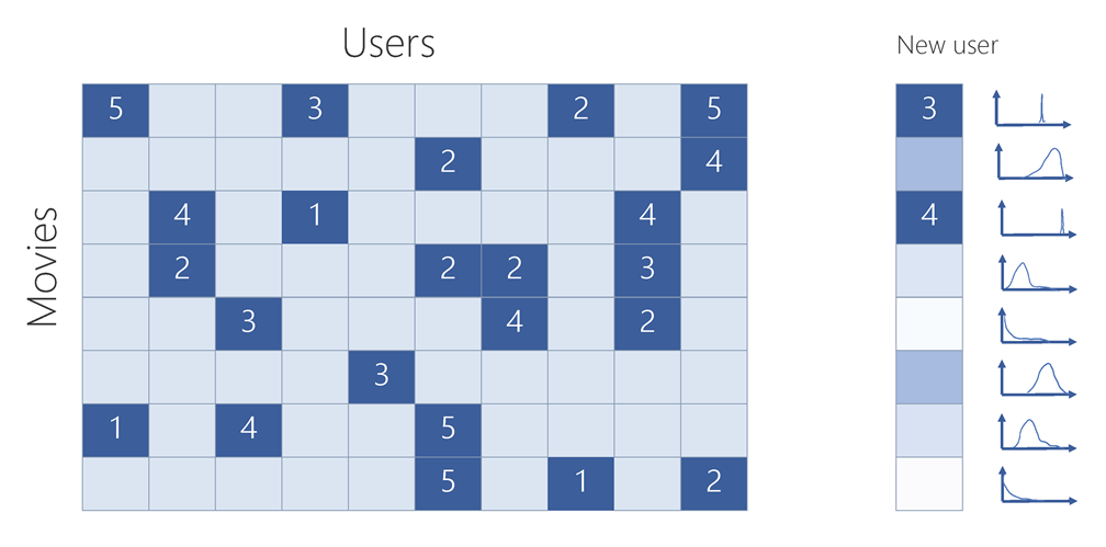
Figure 2-11. Streaming service: movie recommendation

Figure 2-12. Automated ML: machine learning pipeline recommendation

As indicated by the distributions shown on the right side of Figures 2-11 and 2-12, automated ML also takes uncertainty into account, incorporating a probabilistic model to determine the best pipeline to try next. This approach allows automated ML to explore the most promising possibilities without exhaustive search, and to converge on the best pipelines for the user’s data faster than competing brute-force approaches.

Preserving Privacy

Automated ML accomplishes all this without having to see the users’ data, preserving privacy. As shown in Figure 2-13, users’ data and execution of the machine learning pipeline both reside in the users’ cloud subscription (or their local machine), for which they have complete control. Only the model performance metrics of each pipeline run are sent back to the automated ML service, which then makes an intelligent, probabilistic choice of which pipelines should be tried next.

Automated ML’s probabilistic model has been trained by running hundreds of millions of experiments, each involving evaluation of a specific pipeline on a given dataset. This training now allows the automated ML service to find good solutions quickly for new problems. And the model continues to learn and improve as it runs on new machine learning tasks—even though, as just mentioned, it does not see users’ data.

Figure 2-13. Preserving privacy

Enabling Transparency

Transparency is important for data scientists as well as other users so that they can understand what’s going on, and trust the output. This is especially crucial for enterprises to use in business-critical scenarios in production.

Automated ML’s heavy focus on transparency makes it easy to understand the produced machine learning pipelines, including all of the stages discussed in the previous section (e.g., data understanding, feature engineering, model selection/optimization). Users can either directly use the machine learning pipeline produced or they can customize it further.

Another aspect of transparency is to understand how the input features contribute to the outcome of the model, also known as model explainability or interpretability. Automated ML makes this easy by offering a feature importance capability. Figure 2-14 shows an example of a customer churn model for which the SupportIncidents count is the top contributing feature. This makes sense because if a customer has had a lot of support issues, the likelihood of them churning is much higher.

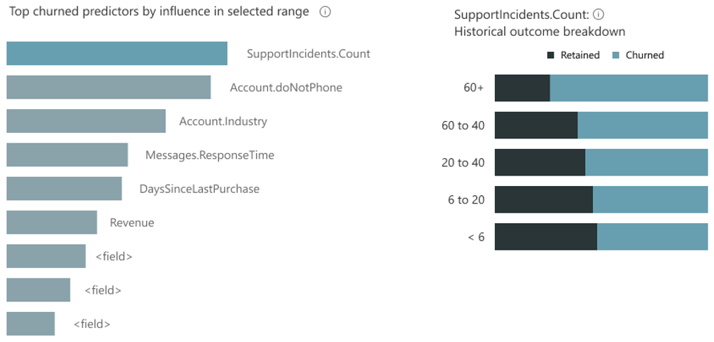
Figure 2-14. Feature importance

Guardrails

In addition to providing transparency, automated ML on Azure also offers guardrails to help users understand potential issues with their data (e.g., missing values, class imbalance) or models and help take corrective actions for improved results. We go into more detail about this in Chapter 7.

End-to-End Model Life-Cycle Management

Automated ML, being a capability of Azure Machine Learning, offers end-to-end (E2E) model life-cycle management, including easy deployment, monitoring, drift analysis, and retraining through integration with ML operationalization (MLOps) capability of Azure Machine Learning. Figure 2-15 shows this E2E flow.

Figure 2-15. E2E model life-cycle management

Conclusion

In this chapter, you learned what Automated Machine Learning is, generally speaking, and how it can help with every stage of building a good machine learning model to solve real-world problems. We also provided a brief overview of how the Azure Machine Learning capability, automated ML, works behind the scenes to build good machine learning models and enable trust by allowing transparency and preserving data privacy.

In subsequent chapters, we’ll cover different aspects of what we touched upon here, and provide hands-on practice and sample scenarios to help you use automated ML in your work.