II
The Discrete Channel with Noise
11. Representation of a Noisy Discrete Channel
We now consider the case where the signal is perturbed by noise during transmission or at one or the other of the terminals. This means that the received signal is not necessarily the same as that sent out by the transmitter. Two cases may be distinguished. If a particular transmitted signal always produces the same received signal, i.e., the received signal is a definite function of the transmitted signal, then the effect may be called distortion. If this function has an inverse—no two transmitted signals producing the same received signal—distortion may be corrected, at least in principle, by merely performing the inverse functional operation on the received signal.
The case of interest here is that in which the signal does not always undergo the same change in transmission. In this case we may assume the received signal E to be a function of the transmitted signal S and a second variable, the noise N.
E = f (S,N)
The noise is considered to be a chance variable just as the message was above. In general it may be represented by a suitable stochastic process. The most general type of noisy discrete channel we shall consider is a generalization of the finite state noise-free channel described previously. We assume a finite number of states and a set of probabilities
pα,i(β,j).
This is the probability, if the channel is in state α and symbol i is transmitted, that symbol j will be received and the channel left in state β. Thus α and β range over the possible states, i over the possible transmitted signals and j over the possible received signals. In the case where successive symbols are independently perturbed by the noise there is only one state, and the channel is described by the set of transition probabilities pi(j), the probability of transmitted symbol i being received as j.
If a noisy channel is fed by a source there are two statistical processes at work: the source and the noise. Thus there are a number of entropies that can be calculated. First there is the entropy H(x) of the source or of the input to the channel (these will be equal if the transmitter is non-singular). The entropy of the output of the channel, i.e., the received signal, will be denoted by H (y). In the noiseless case H(y) = H(x). The joint entropy of input and output will be H(x,y). Finally there are two conditional entropies Hx(y) and Hy(x), the entropy of the output when the input is known and conversely. Among these quantities we have the relations
H(x,y) = H(x) + Hx(y) = H(y) + Hy(x).
All of these entropies can be measured on a per-second or a per-symbol basis.
12. Equivocation and Channel Capacity
If the channel is noisy it is not in general possible to reconstruct the original message or the transmitted signal with certainty by any operation on the received signal E. There are, however, ways of transmitting the information which are optimal in combating noise. This is the problem which we now consider.
Suppose there are two possible symbols 0 and 1, and we are transmitting at a rate of 1000 symbols per second with probabilities p0 = p1 =  . Thus our source is producing information at the rate of 1000 bits per second. During transmission the noise introduces errors so that, on the average, 1 in 100 is received incorrectly (a 0 as 1, or 1 as 0). What is the rate of transmission of information? Certainly less than 1000 bits per second since about 1% of the received symbols are incorrect. Our first impulse might be to say the rate is 990 bits per second, merely subtracting the expected number of errors. This is not satisfactory since it fails to take into account the recipient's lack of knowledge of where the errors occur. We may carry it to an extreme case and suppose the noise so great that the received symbols are entirely independent of the transmitted symbols. The probability of receiving 1 is whatever was transmitted and similarly for 0. Then about half of the received symbols are correct due to chance alone, and we would be giving the system credit for transmitting 500 bits per second while actually no information is being transmitted at all. Equally “good” transmission would be obtained by dispensing with the channel entirely and flipping a coin at the receiving point.
Evidently the proper correction to apply to the amount of information transmitted is the amount of this information which is missing in the received signal, or alternatively the uncertainty when we have received a signal of what was actually sent. From our previous discussion of entropy as a measure of uncertainty it seems reasonable to use the conditional entropy of the message, knowing the received signal, as a measure of this missing information. This is indeed the proper definition, as we shall see later. Following this idea the rate of actual transmission, R, would be obtained by subtracting from the rate of production (i.e., the entropy of the source) the average rate of conditional entropy.
R = H(x) — Hy(x)
The conditional entropy Hy(x) will, for convenience, be called the equivocation. It measures the average ambiguity of the received signal.
In the example considered above, if a 0 is received the a posteriori probability that a 0 was transmitted is .99, and that a 1 was transmitted is .01. These figures are reversed if a 1 is received. Hence
Hy(x) = — [.99 log .99 + 0.01 log 0.01]
= .081 bits/symbol
or 81 bits per second. We may say that the system is transmitting at a rate 1000 — 81 = 919 bits per second. In the extreme case where a 0 is equally likely to be received as a 0 or 1 and similarly for 1, the a posteriori probabilities are , and
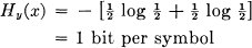
or 1000 bits per second. The rate of transmission is then 0 as it should be.
The following theorem gives a direct intuitive interpretation of the equivocation and also serves to justify it as the unique appropriate measure. We consider a communication system and an observer (or auxiliary device) who can see both what is sent and what is recovered (with errors due to noise). This observer notes the errors in the recovered message and transmits data to the receiving point over a “correction channel” to enable the receiver to correct the errors. The situation is indicated schematically in Fig. 8.
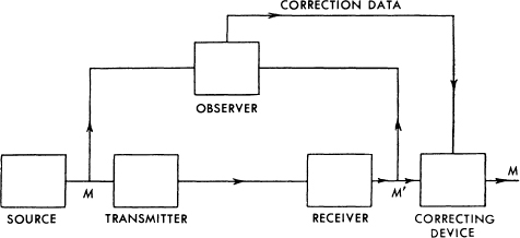
Fig. 8.—Schematic diagram of a correction system.
Theorem 10: If the correction channel has a capacity equal to Hy(x) it is possible to so encode the correction data as to send it over this channel and correct all but an arbitrarily small fraction ∊ of the errors. This is not possible if the channel capacity is less than Hy(x).
Roughly then, Hy(x) is the amount of additional information that must be supplied per second at the receiving point to correct the received message.
To prove the first part, consider long sequences of received message M′ and corresponding original message M. There will be logarithmically THy (x) of the M's which could reasonably have produced each M′. Thus we have THy(x) binary digits to send each T seconds. This can be done with ∊ frequency of errors on a channel of capacity Hy(x).
The second part can be proved by noting, first, that for any discrete chance variables x, y, z
Hy(x, z) ≥ Hy(x).
The left-hand side can be expanded to give
Hy(z) + Hyz(x) ≥ Hy(x)
Hyz(x) ≥ Hy(x) — Hy(z) ≥ Hy(x) — H(z).
If we identify x as the output of the source, y as the received signal and z as the signal sent over the correction channel, then the right-hand side is the equivocation less the rate of transmission over the correction channel. If the capacity of this channel is less than the equivocation the right-hand side will be greater than zero and Hyz(x) > 0. But this is the uncertainty of what was sent, knowing both the received signal and the correction signal. If this is greater than zero the frequency of errors cannot be arbitrarily small.
Example:
Suppose the errors occur at random in a sequence of binary digits: probability p that a digit is wrong and q = 1 — p that it is right. These errors can be corrected if their position is known. Thus the correction channel need only send information as to these positions. This amounts to transmitting from a source which produces binary digits with probability p for 1 (incorrect) and q for 0 (correct). This requires a channel of capacity
—[p log p + q log q]
which is the equivocation of the original system.
The rate of transmission R can be written in two other forms due to the identities noted above. We have
R = H(x) — Hy(x)
= H(y) — Hx(y)
= H(x) + H(y) — H(x, y).
The first defining expression has already been interpreted as the amount of information sent less the uncertainty of what was sent. The second measures the amount received less the part of this which is due to noise. The third is the sum of the two amounts less the joint entropy and therefore in a sense is the number of bits per second common to the two. Thus all three expressions have a certain intuitive significance.
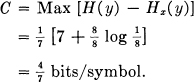
The capacity C of a noisy channel should be the maximum possible rate of transmission, i.e., the rate when the source is properly matched to the channel. We therefore define the channel capacity by
C = Max (H(x) — Hy(x))
where the maximum is with respect to all possible information sources used as input to the channel. If the channel is noiseless, Hy(x) = 0. The definition is then equivalent to that already given for a noiseless channel since the maximum entropy for the channel is its capacity by Theorem 8.
13. The Fundamental Theorem for a Discrete Channel with Noise
It may seem surprising that we should define a definite capacity C for a noisy channel since we can never send certain information in such a case. It is clear, however, that by sending the information in a redundant form the probability of errors can be reduced. For example, by repeating the message many times and by a statistical study of the different received versions of the message the probability of errors could be made very small. One would expect, however, that to make this probability of errors approach zero, the redundancy of the encoding must increase indefinitely, and the rate of transmission therefore approach zero. This is by no means true. If it were, there would not be a very well defined capacity, but only a capacity for a given frequency of errors, or a given equivocation; the capacity going down as the error requirements are made more stringent. Actually the capacity C defined above has a very definite significance. It is possible to send information at the rate C through the channel with as small a frequency of errors or equivocation as desired by proper encoding. This statement is not true for any rate greater than C. If an attempt is made to transmit at a higher rate than C, say C + R1, then there will necessarily be an equivocation equal to or greater than the excess R1. Nature takes payment by requiring just that much uncertainty, so that we are not actually getting any more than C through correctly.
The situation is indicated in Fig. 9. The rate of information into the channel is plotted horizontally and the equivocation vertically. Any point above the heavy line in the shaded region can be attained and those below cannot. The points on the line cannot in general be attained, but there will usually be two points on the line that can.
These results are the main justification for the definition of C and will now be proved.
Theorem 11: Let a discrete channel have the capacity C and a discrete source the entropy per second H. If H ≤ C there exists a coding system such that the output of the source can be transmitted over the channel with an arbitrarily small frequency of errors (or an arbitrarily small equivocation). If H > C it is possible to encode the source so that the equivocation is less than H — C + ∊ where ∊ is arbitrarily small. There is no method of encoding which gives an equivocation less than H — C.
The method of proving the first part of this theorem is not by exhibiting a coding method having the desired properties, but by showing that such a code must exist in a certain group of codes.
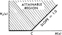
Fig. 9.—The equivocation possible for a given input entropy to a channel.
In fact we will average the frequency of errors over this group and show that this average can be made less than ∊. If the average of a set of numbers is less than ∊ there must exist at least one in the set which is less than ∊. This will establish the desired result.
The capacity C of a noisy channel has been defined as
C = Max (H(x) — Hy(x))
where x is the input and y the output. The maximization is over all sources which might be used as input to the channel.
Let S0 be a source which achieves the maximum capacity C. If this maximum is not actually achieved by any source (but only approached as a limit) let S0 be a source which approximates to giving the maximum rate. Suppose S0 is used as input to the channel. We consider the possible transmitted and received sequences of a long duration T. The following will be true:
1. The transmitted sequences fall into two classes, a high probability group with about 2TH(x) members and the remaining sequences of small total probability.
2. Similarly the received sequences have a high probability set of about 2TH(y) members and a low probability set of remaining sequences.
3. Each high probability output could be produced by about 2THy(x) inputs. The total probability of all other cases is small.
4. Each high probability input could result in about 2THx(y) outputs. The total probability of all other results is small.
All the ∊'s and δ's implied by the words “small” and “about” in these statements approach zero as we allow T to increase and S0 to approach the maximizing source.
The situation is summarized in Fig. 10 where the input sequences are points on the left and output sequences points on the right. The upper fan of cross lines represents the range of possible causes for a typical output. The lower fan represents the range of possible results from a typical input. In both cases the “small probability” sets are ignored.
Now suppose we have another source S, producing information at rate R with R < C. In the period T this source will have 2TR high probability messages. We wish to associate these with a selection of the possible channel inputs in such a way as to get a small frequency of errors. We will set up this association in all possible ways (using, however, only the high probability group of inputs as determined by the source S0) and average the frequency of errors for this large class of possible coding systems. This is the same as calculating the frequency of errors for a random association of the messages and channel inputs of duration T. Suppose a particular output y1 is observed. What is the probability of more than one message from S in the set of possible causes of y1? There are 2TR messages distributed at random in 2TH(x) points. The probability of a particular point being a message is thus
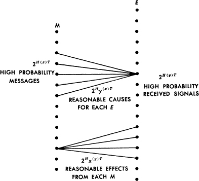
Fig. 10.—Schematic representation of the relations between inputs and outputs in a channel.
2T (R–H (x)).
The probability that none of the points in the fan is a message (apart from the actual originating message) is
P = [1 — 2T (R — H(x))]2THy(x).
Now R < H(x) — Hy(x) so R — H(x) = — Hy(x) — η with η positive. Consequently
P = [1 — 2–THy(x)–Tη]2THy(x)
approaches (as T → ∞)
1 — 2-Tη.
Hence the probability of an error approaches zero and the first part of the theorem is proved.
The second part of the theorem is easily shown by noting that we could merely send C bits per second from the source, completely neglecting the remainder of the information generated. At the receiver the neglected part gives an equivocation H(x) — C and the part transmitted need only add ∊. This limit can also be attained in many other ways, as will be shown when we consider the continuous case.
The last statement of the theorem is a simple consequence of our definition of C. Suppose we can encode a source with H(x) = C + a in such a way as to obtain an equivocation Hy(x) = a — ∊ with ∊ positive. Then
H(x) — Hy(x) = C + ∊
with ∊ positive. This contradicts the definition of C as the maximum of H(x) — Hy(x).
Actually more has been proved than was stated in the theorem. If the average of a set of positive numbers is within ∊ of zero, a fraction of at most  can have values greater than . Since ∊ is arbitrarily small we can say that almost all the systems are arbitrarily close to the ideal.
14. Discussion
The demonstration of Theorem 11, while not a pure existence proof, has some of the deficiencies of such proofs. An attempt to obtain a good approximation to ideal coding by following the method of the proof is generally impractical. In fact, apart from some rather trivial cases and certain limiting situations, no explicit description of a series of approximation to the ideal has been found. Probably this is no accident but is related to the difficulty of giving an explicit construction for a good approximation to a random sequence.
An approximation to the ideal would have the property that if the signal is altered in a reasonable way by the noise, the original can still be recovered. In other words the alteration will not in general bring it closer to another reasonable signal than the original. This is accomplished at the cost of a certain amount of redundancy in the coding. The redundancy must be introduced in the proper way to combat the particular noise structure involved. However, any redundancy in the source will usually help if it is utilized at the receiving point. In particular, if the source already has a certain redundancy and no attempt is made to eliminate it in matching to the channel, this redundancy will help combat noise. For example, in a noiseless telegraph channel one could save about 50% in time by proper encoding of the messages. This is not done and most of the redundancy of English remains in the channel symbols. This has the advantage, however, of allowing considerable noise in the channel. A sizable fraction of the letters can be received incorrectly and still reconstructed by the context. In fact this is probably not a bad approximation to the ideal in many cases, since the statistical structure of English is rather involved and the reasonable English sequences are not too far (in the sense required for the theorem) from a random selection.
As in the noiseless case a delay is generally required to approach the ideal encoding. It now has the additional function of allowing a large sample of noise to affect the signal before any judgment is made at the receiving point as to the original message. Increasing the sample size always sharpens the possible statistical assertions.
The content of Theorem 11 and its proof can be formulated in a somewhat different way which exhibits the connection with the noiseless case more clearly. Consider the possible signals of duration T and suppose a subset of them is selected to be used. Let those in the subset all be used with equal probability, and suppose the receiver is constructed to select, as the original signal, the most probable cause from the subset, when a perturbed signal is received. We define N(T, q) to be the maximum number of signals we can choose for the subset such that the probability of an incorrect interpretation is less than or equal to q.
Theorem 12: 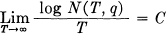 , where C is the channel capacity, provided that q does not equal 0 or 1.
In other words, no matter how we set our limits of reliability, we can distinguish reliably in time T enough messages to correspond to about CT bits, when T is sufficiently large. Theorem 12 can be compared with the definition of the capacity of a noiseless channel given in section 1.
15. Example of a Discrete Channel and Its Capacity
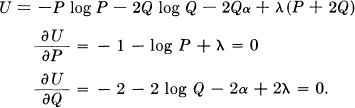
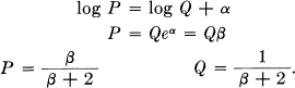
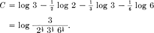
A simple example of a discrete channel is indicated in Fig. 11. There are three possible symbols. The first is never affected by noise. The second and third each have probability p of coming through undisturbed, and q of being changed into the other of the pair. Let α = — [p log p + q log q] and let P, Q and Q be the probabilities of using the first, second and third symbols respectively (the last two being equal from consideration of symmetry). We have:

Fig. 11.—Example of a discrete channel.
H(x) = — P log P — 2Q log Q
Hy(x) = 2Qα.
We wish to choose P and Q in such a way as to maximize H(x) — Hy(x), subject to the constraint P + 2Q = 1. Hence we consider
Eliminating λ
The channel capacity is then
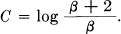
Note how this checks the obvious values in the cases p = 1 and p = . In the first, β = 1 and C = log 3, which is correct since the channel is then noiseless with three possible symbols. If p = , β = 2 and C = log 2. Here the second and third symbols cannot be distinguished at all and act together like one symbol. The first symbol is used with probability P = and the second and third together with probability .This may be distributed between them in any desired way and still achieve the maximum capacity.
For intermediate values of p the channel capacity will lie between log 2 and log 3. The distinction between the second and third symbols conveys some information but not as much as in the noiseless case. The first symbol is used somewhat more frequently than the other two because of its freedom from noise.
16. The Channel Capacity in Certain Special Cases
If the noise affects successive channel symbols independently it can be described by a set of transition probabilities pij. This is the probability, if symbol i is sent, that j will be received. The channel capacity is then given by the maximum of
where we vary the Pi subject to ΣPi = 1. This leads by the method of Lagrange to the equations,
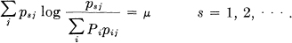
Multiplying by Ps and summing on s shows that μ = — C. Let the inverse of psj (if it exists) be hst so that  . Then:

Hence:

or,

This is the system of equations for determining the maximizing values of Pi, with C to be determined so that ΣPi = 1. When this is done C will be the channel capacity, and the Pi the proper probabilities for the channel symbols to achieve this capacity.
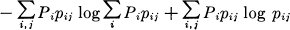
If each input symbol has the same set of probabilities on the lines emerging from it, and the same is true of each output symbol, the capacity can be easily calculated. Examples are shown in Fig. 12. In such a case Hx(y) is independent of the distribution of probabilities on the input symbols, and is given by — Σ pi log pi where the pi are the values of the transition probabilities from any input symbol. The channel capacity is
Fig. 12.—Examples of discrete channels with the same transition probabilities for each input and for each output.
Max [H(y) — Hx(y)]
= Max H(y) + Σ pi log pi.
The maximum of H(y) is clearly log m where m is the number of output symbols, since it is possible to make them all equally probable by making the input symbols equally probable. The channel capacity is therefore
C = log m + Σ pi log pi.
In Fig. 12a it would be
C = log 4 — log 2 = log 2.
This could be achieved by using only the 1st and 3d symbols. In Fig. 12b
In Fig. 12c we have
Suppose the symbols fall into several groups such that the noise never causes a symbol in one group to be mistaken for a symbol in another group. Let the capacity for the nth group be Cn (in bits per second) when we use only the symbols in this group. Then it is easily shown that, for best use of the entire set, the total probability Pn of all symbols in the nth group should be

Within a group the probability is distributed just as it would be if these were the only symbols being used. The channel capacity is
C = log Σ2Cn.
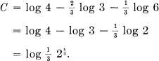
17. An Example of Efficient Coding
The following example, although somewhat artificial, is a case in which exact matching to a noisy channel is possible. There are two channel symbols, 0 and 1, and the noise affects them in blocks of seven symbols. A block of seven is either transmitted without error, or exactly one symbol of the seven is incorrect. These eight possibilities are equally likely. We have
An efficient code, allowing complete correction of errors and transmitting at the rate C, is the following (found by a method due to R. Hamming) :
Let a block of seven symbols be X1 X2,…, X7. Of these X3, X5, X6 and X7 are message symbols and chosen arbitrarily by the source. The other three are redundant and calculated as follows:
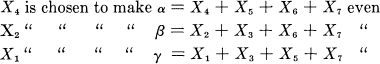
When a block of seven is received α, β and γ are calculated and if even called zero, if odd called one. The binary number α β γ then gives the subscript of the Xi that is incorrect (if 0 there was no error) .10
10 For some further examples of self-correcting codes see M. J. E. Golay, “Notes on Digital Coding,” Proceedings of the Institute of Radio Engineers, v. 37, No. 6, June, 1949, p. 637.