Chapter 13
Understanding heat and groundwater flow through continental flood basalt provinces: insights gained from alternative models of permeability/depth relationships for the Columbia Plateau, United States
Erick R. Burns1, Colin F. Williams2, Steven E. Ingebritsen2, Clifford I. Voss2, Frank A. Spane3 and Jacob DeAngelo2
1U.S. Geological Survey, Portland, OR, USA; 2U.S. Geological Survey, Menlo Park, CA, USA; 3Pacific Northwest National Laboratory, Richland, WA, USA
Abstract
Heat-flow mapping of the western United States has identified an apparent low-heat-flow anomaly coincident with the Columbia Plateau Regional Aquifer System, a thick sequence of basalt aquifers within the Columbia River Basalt Group. A heat and mass transport model was used to evaluate the potential impact of groundwater flow on heat flow along two different regional groundwater flow paths. Limited in situ permeability (k) data from the Columbia River Basalt Group are compatible with a steep permeability decrease (approximately 3.5 orders of magnitude) at 600–900m depth and approximately 40°C. Numerical simulations incorporating this permeability decrease demonstrate that regional groundwater flow can explain lower-than-expected heat flow in these highly anisotropic (kx/kz ∼104) continental flood basalts. Simulation results indicate that the abrupt reduction in permeability at approximately 600m depth results in an equivalently abrupt transition from a shallow region where heat flow is affected by groundwater flow to a deeper region of conduction-dominated heat flow. Most existing heat-flow measurements within the Columbia River Basalt Group are from shallower than 600m depth or near regional groundwater discharge zones, so that heat-flow maps generated using these data are likely influenced by groundwater flow. Substantial k decreases at similar temperatures have also been observed in the volcanic rocks of the adjacent Cascade Range volcanic arc and at Kilauea Volcano, Hawaii, where they result from low-temperature hydrothermal alteration.
Key words: advection, advective heat transport, anisotropy, conduction-dominated, flood basalts, heat flow, hydrothermal alteration, permeability, regional groundwater flow
Introduction
Within the Earth's upper crust, heat flow occurs via two primary mechanisms, conduction and advection (commonly by groundwater). Heat-flow maps (e.g., Fig. 13.1) are derived from the vertical component of heat flow measured in a borehole and are typically intended to represent the conductive component of heat flow from the Earth's upper crust. In areas where there is significant advection of heat, shallow heat-flow measurements may not reflect thermal conditions deeper in the crust.
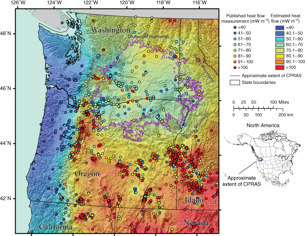
Fig. 13.1 Heat-flow map of the northwestern United States showing apparent low heat flow in the vicinity of the Columbia Plateau Regional Aquifer System. Contours are based on published heat-flow data for the Cascade Range and adjacent regions assembled for the USGS geothermal database. The map was constructed using the methods of Williams & DeAngelo (2008). The Approximate Extent of Columbia Plateau Regional Aquifer System is the extent of Columbia River Basalts from the geologic model of Burns et al. (2011). (See color plate section for the color representation of this figure.)
Advective heat transport can be driven by forced convection and free convection (Saar 2011). Free convection refers to density-driven flow, and forced convection refers to groundwater flow driven by hydraulic gradients resulting from topography and other factors. Free convection results from unstable fluid-density configurations and depends on the ease with which the fluid can move through the geologic material, the rate of heat addition, and the rate at which heat is conducted away from the heat source. The Rayleigh number is a measure of the relation between these factors, and free convection occurs when the Rayleigh number exceeds a critical value. In natural systems, both free convection and forced convection can influence groundwater flow patterns.
The hydrogeologic relation between heat flow and fluid flow has been the topic of considerable research, which is summarized in review articles by Anderson (2005) and Saar (2011). Cross-sectional numerical models have been used to demonstrate thermal anomalies associated with active groundwater flow (e.g., Smith & Chapman 1983; Forster & Smith 1988a,b, 1989; Nunn & Deming 1991; Deming 1993). Early work by Smith & Chapman (1983) demonstrated most of the salient features and dependencies for systems with no free convection. Compared to pure heat conduction through an aquifer system, advective transport of heat results in a decrease in temperature and near-surface heat flow in upland recharge areas and an increase in temperature and near-surface heat flow in lowland discharge areas. Using reasonable hydrogeologic parameters, temperature and heat-flow distributions have been shown to be sensitive to variations in recharge and discharge magnitude and location, depth and length of the aquifer system, and permeability.
Recent regional mapping of geothermal resources of the western United States (e.g., Williams & DeAngelo 2008, 2011) identified an apparent low-heat-flow anomaly associated with the Columbia Plateau Regional Aquifer System (Fig. 13.1). Although heat flow in most areas immediately to the east of the Cascade Range is above the global average for Cenozoic tectonic provinces (approximately >65 mW m−2; Pollack et al. 1993), heat-flow measurements from most of the Columbia Plateau are significantly lower. Low heat flow through the Columbia Plateau is particularly enigmatic because this province is seismically active and lies adjacent to active volcanoes of the Cascade Range. However, throughout the Columbia Plateau, most temperature profile data used to measure heat flow have been collected from depth intervals that are within the active regional groundwater flow system (typically <500 m deep, Fig. 13.2).
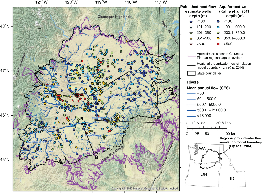
Fig. 13.2 Map of compiled borehole temperature logs (stars) and aquifer tests from groundwater supply wells (circles). The bottom of each temperature log is frequently at or above the depth of nearby aquifer tests, indicating that most temperature data were collected within the active groundwater system. To estimate intrinsic permeability from aquifer tests, the temperature of water pumped was estimated using the nearest temperature log. Representative cross sections A–A′ and B–B′ were used for coupled groundwater and heat-flow simulations. (See color plate section for the color representation of this figure.)
In order to understand geothermal heat flow at the province scale, it is necessary to understand the permeability structure of the upper crust and the resulting coupled heat and groundwater flow. The Columbia Plateau Regional Aquifer System is comprised almost entirely of continental flood basalts, a type example of large igneous provinces (Jerram & Widdowson 2005) typified by thick and laterally extensive mafic lava flows. The massive sheet flows of the Columbia Plateau result in confined aquifers over much of the region, but individual lobe-shaped flows of smaller areal extent or frequent joints and fractures can result in unconfined aquifers. This study and previous studies agree that the permeability of the Columbia River Basalt Group – and presumably other continental flood basalts – is highly anisotropic (kx/kz ∼104). The thinner, less laterally extensive basalt flows of the adjacent Cascade Range (Manga 1996, 1997) and the Hawaiian Islands (e.g., Gingerich & Voss 2005) exhibit much less anisotropy (kx/kz ≤ 102).
This manuscript summarizes two-dimensional (2D) cross-sectional coupled groundwater and heat-flow models that demonstrate that, for the most likely distributions of permeability and aquifer tests (Kahle et al. 2011; Spane 2013), the apparent low-heat-flow anomaly in the Columbia Plateau Regional Aquifer System can be explained by accounting for the heat transported to large regional rivers by the groundwater system. The heat-flow pattern is shown to be spatially complex both laterally and vertically, illustrating the difficulties in using the current borehole temperature data set to estimate regional heat flow.
Background
Location and geology of study area
The Columbia Plateau Regional Aquifer System lies in a structural and topographic basin within the Columbia River drainage. It is bounded on the west by the Cascade Range, on the east by the Rocky Mountains, on the north by the Okanogan Highlands, and on the south by the Blue Mountains (Fig. 13.1). The Columbia Plateau is underlain by the Miocene Columbia River Basalt Group, a series of more than 300 sheet and intracanyon lava flows and sedimentary interbeds. Sheet flows are areally extensive, sometimes covering tens of thousands of square kilometers. Flows that separate into lobes or channels controlled by paleotopography are called intracanyon flows. Sheet flows commonly take on intracanyon character near their margins. Individual flows range in thickness from 3 m to more than 100 m (Tolan et al. 1989; Drost et al. 1990). Near the center of the Columbia Plateau Regional Aquifer System, the total thickness of the Columbia River Basalt Group is estimated to exceed 5 km (Reidel et al. 2002; Burns et al. 2011). Thick sedimentary deposits overlie the basalt in only a few basins, with basalt units occurring at or near land surface over most of the Plateau (Burns et al. 2011). Columbia River Basalt Group units are variably folded and faulted. Generally, structural intensity is greater near the uplifted Blue Mountains and Cascade Range. An expanded description of the Columbia River Basalt Group is provided by Reidel et al. (2013).
Groundwater occurrence and movement
Groundwater moves through the regional aquifer system along preferential pathways developed during lava deposition. Most Columbia River Basalt Group lava flows consist of a dense flow interior and irregular flow tops and flow bottoms with a variety of textures (Reidel et al. 2002). Although flow interiors have joints and fractures, they typically do not transmit water easily. Flow tops and bottoms are commonly vesicular or brecciated, and may or may not be permeable. Local permeability of flow tops and bottoms can be highly variable over short distances as a result of depositional processes, but tends to be high over long distances, resulting in highly transmissive aquifers at the regional scale. The Columbia River Basalt Group thus comprises a stack of laterally extensive lava flows with relatively thin permeable productive zones at flow tops and flow bottoms separated by relatively thick dense flow interiors of low permeability. Thin permeable aquifers are estimated to occupy about 10% of the total flow thickness (Burns et al. 2012a; Ely et al. 2014). Flow interiors have low permeability and low storage characteristics, so that they form effective confining units between permeable flow tops. As a result, the aquifer system is highly anisotropic, with effective horizontal hydraulic conductivity controlled by the fraction of the thickness occupied by thin aquifers and the effective vertical hydraulic conductivity controlled by the dense flow interiors. Effective bulk horizontal permeability is frequently more than 104 times greater than bulk vertical permeability (summary Tables 2–4 of Kahle et al. 2011). Flow interiors also commonly have negligible porosity compared to an approximate value of 0.25 for thin aquifers (Reidel et al. 2002). The bulk porosity of the Columbia River Basalt Group is about 0.025.
The limited data available suggest that horizontal hydraulic conductivity may decrease with increasing depth. Hansen et al. (1994) simulated groundwater flow through the entire thickness of the Columbia Plateau Regional Aquifer System, but during model calibration, it was found that horizontal hydraulic conductivity (Kh) values decreased with increasing depth. To correct for the reduction in permeability with depth, the equations of Weiss (1982) were used, under the assumption that Kh would decrease as a function of overburden pressure only, resulting in a typical reduction in permeability by a factor <2 over the entire thickness. Recent simulation of the Columbia Plateau Regional Aquifer System (Ely et al. 2014) tested the hypothesis that horizontal permeability decreases with increasing depth using computer-assisted parameter estimation techniques, but found that the calibration data were insufficient to positively identify a persistent vertical trend in permeability. This was attributed to the fact that almost all of the calibration data were collected from very shallow depths compared to the total thickness of the Columbia Plateau Regional Aquifer System, so that model calibration was only sensitive to the upper part of the groundwater flow system. It was postulated that the Hansen and Vaccaro model may have required a vertical trend in permeability to compensate for model structural error. In particular, the Hansen and Vaccaro model had very coarse vertical discretization (cells were hundreds to thousands of meters thick) compared to the Ely et al. model (cells were typically 30 m thick), possibly resulting in lowering of permeability during calibration to reduce erroneous overconnection of the deep aquifers with surface water boundaries. Hansen et al. (1994) estimated that Columbia River Basalt Group bulk Kh ranges from 3.0 × 10⁻⁷ to 3.0 × 10⁻⁵ m s−1, and Ely et al. (2014) estimated that Columbia River Basalt Group bulk Kh ranges from 3.5 × 10⁻⁶ to 9.9 × 10⁻⁵ m s−1. Both studies found that Kh varies laterally, with lower Kh occurring in areas with more intense geologic structure (more folds and faults) and higher Kh in relatively undeformed areas.
Published Kh values from hydraulic tests for Columbia River Basalt Group units range from 10−15 to 0.21 m s−1, over 14 orders of magnitude (Kahle et al. 2011). These tests include both lava interflows (aquifers) and flow interiors (confining units). The Kh estimates from aquifer pump tests documented a narrower range of Kh of 2.8 × 10⁻⁷ to 0.21 m s−1. Near the center of the Columbia Plateau Regional Aquifer System, Spane (1982) found that hydraulic conductivity in the deeper Grande Ronde Basalts tended to be 2–3 orders of magnitude lower than that in the overlying Saddle Mountains and Wanapum Basalts. However, the Grande Ronde Basalt does not have uniformly lower Kh values throughout the Columbia Plateau Regional Aquifer System (plate 6 of Hansen et al. 1994; Ely et al. 2014), indicating that the reduction in permeability observed by Spane (1982) may be related to depth, temperature, and the degree of secondary mineralization, which all increase along the deep groundwater flow paths near the center of the basin (Reidel et al. 2002).
Changes in lithology associated with folds and faults also affect flow paths through the Columbia Plateau Regional Aquifer System by forming flow barriers or preferential pathways for groundwater flow (Newcomb 1959; Porcello et al. 2009; Snyder & Haynes 2010; Kahle et al. 2011; Burns et al. 2012a,b). Faults create flow barriers by juxtaposing thin aquifers with flow interiors; furthermore, fault gouge consists largely of low-permeability clay-rich minerals. At the regional scale, geologic structure apparently has the net effect of reducing the effective horizontal hydraulic conductivity. As a result, regional modeling efforts suggest lower horizontal hydraulic conductivity than the values reported from aquifer tests (e.g., Hansen et al. 1994; Kahle et al. 2011). Similarly, modeling efforts result in higher predicted vertical hydraulic conductivity (e.g., Hansen et al. 1994) than the values suggested by aquifer tests on basalt flow interiors (e.g., Long et al. 1982b) because vertical connectivity at the regional scale is also controlled by the geometry of individual lava flows, allowing water to flow through the vertical stack of lavas via preferred pathways.
Groundwater flows through thin aquifers from the uplands toward large regional rivers, entering aquifers preferentially in the uplands where precipitation is higher and lava flow margins are exposed (typical aquifer geometries shown in Fig. 13.3). The older lava flows tend to be more voluminous and areally extensive and have also undergone more deformation, forming structural and erosional troughs into which younger, less-voluminous flows were deposited (Fig. 13.3). Some deeper aquifers may be completely covered by younger lava flows (Fig. 13.3), restricting recharge.
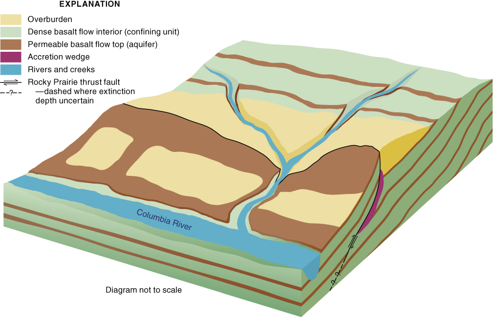
Fig. 13.3 Conceptual model of aquifer system geometry (from Burns et al. 2012a). Upland recharge can enter thin aquifers at flow margins. Geologic structures can act as flow barriers that may or may not crosscut all aquifers. (See color plate section for the color representation of this figure.)
Groundwater exits the aquifers into rivers and streams. The strongest control on hydraulic head in any Columbia River Basalt Group aquifer is often the lowest elevation at which the aquifer intersects the land surface (Burns et al. 2012a). Thus, if an aquifer intersects a large regional river, hydraulic head in that aquifer may be similar to hydraulic head in that river. If there is a flow barrier between an aquifer and the large regional rivers, then the aquifer may discharge at higher elevations where upland streams intersect the aquifer (Fig. 13.3). Groundwater that bypasses the stream–aquifer intersection has poor connection with discharge locations and may be very old, while water that seasonally fills and drains from the upper portions of the aquifer may be much younger. Horizontal head gradients within individual aquifers can be very small in deep, almost stagnant parts of the system, with much steeper gradients in generally shallower, active parts of the system. The steepest gradients (approaching the magnitude and direction of the gradient of the land surface) occur in structurally complex, high-recharge upland areas. This conceptual model explains why water in deep aquifers near the center of the Columbia Plateau is more geochemically evolved (Kahle et al. 2011), and why there is significant groundwater contribution year-round to springs and streams near the crest of the Blue Mountains (the anticlinal ridge covered by Columbia River Basalt Group lavas near the southeastern boundary of the study area).
More detailed descriptions of the Columbia Plateau Regional Aquifer System are provided in reports by Kahle et al. (2009), who discuss the geologic framework; Burns et al. (2011), who describe the 3D characteristics of the geology; and Kahle et al. (2011), who discuss the hydrogeologic framework and the hydrologic budget.
Methods of analysis and results
The SUTRA model (Voss & Provost 2002) was used to perform coupled groundwater and heat-flow simulations. The hypothesis that advective transport of heat can account for the apparently low heat flow under the Columbia Plateau Regional Aquifer System was tested by simulating a constant 80 mW m−2 heat flow at the bottom of the domain and quantifying the effect of advection on the apparent near-surface heat flow. An analysis of existing permeability data was conducted, and three different permeability/depth relations, constrained by these data, were evaluated. Prior to performing SUTRA simulations, a Rayleigh number analysis was performed to evaluate the likelihood that density-driven convective flow occurs in the Columbia Plateau Regional Aquifer System.
Rayleigh analysis
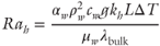
Free convection can occur if the Rayleigh number (Ra) exceeds the critical Rayleigh number (Racrit). For a system with anisotropic permeability and isotropic heat conduction, Phillips (1991, pp. 144–145) derives the following special form of the Raleigh number (Ra) and the associated Racrit.
and
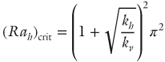
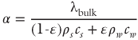
where the relation of the form of the Rayleigh number to the horizontal permeability (kh) has been made explicit and the critical Rayleigh number depends on the ratio of the horizontal-to-vertical permeability  . The characteristic length scale L is the thickness across which a temperature difference (ΔT) is experienced, αw is the thermal expansivity of the fluid phase, ρw is the density of the fluid phase, cw is the heat capacity of the fluid phase, μw is the dynamic viscosity of the fluid, λbulk is the bulk thermal conductivity of the medium, and g is the gravitational constant.
Rah and (Rah)crit were estimated using conservative values for both the upper permeable zone and the thickest part of the Columbia River Basalt Group (approximately 5 km). Because of the large horizontal-to-vertical anisotropy in permeability, in both cases Rah was approximately 100 times less than (Rah)crit indicating that free convection can be ignored during the analysis.
Permeability/depth relations
Rapid reductions in permeability over a narrow depth range have been identified in studies of several volcanic terrains and have generally been attributed to hydrothermal alteration at temperatures above 30 °C. Investigations at geothermal sites throughout the Cascade Range identified a significant decrease in permeability with depth in the range from approximately 200 to 1000 m (e.g., Swanberg et al. 1988; Blackwell 1994; Hulen & Lutz 1999) associated with low-temperature hydrothermal alteration of Cascade Range rocks at temperatures in the range of 30–50 °C (e.g., Bargar & Keith 1999). At the Kilauea Volcano, Hawaii, Keller et al. (1979) attributed a significant reduction in permeability to hydrothermal alteration below 488 m where temperatures increased from 30 to 60 °C over a short interval. Recently published detailed borehole test data (Spane 2013) shows that for several deep boreholes located near the center of the Columbia Plateau Regional Aquifer System, rapid reduction in permeability starts at a similar depth of approximately 600 m. Ely et al. (2014) tested the hypothesis that permeability is significantly less in Columbia River Basalt Group units deeper than 600 m by lowering Kh below this depth by a factor of 1000 and recalibrating their regional model. Model fit was not significantly changed, and shallow groundwater parameters remained within the range of expected values. It was concluded that model calibration was not sensitive to the deep system permeability because most groundwater flows through the upper 600 m, where aquifers are directly connected to recharge and discharge boundaries. In other words, the available hydrogeologic data were insufficient to allow unique estimation of the deep permeability structure of the Columbia Plateau Regional Aquifer System.
Ely et al. (2014) simulated the Columbia Plateau Regional Aquifer System using model cells that were approximately 30 m thick, representing a typical lava flow thickness including the permeable flow top and bottom, and using bulk horizontal and vertical permeability. Locally, effective horizontal permeability is controlled by thin aquifers, while vertical permeability is controlled by the thick flow interiors (confining units). Because individual aquifers are not continuously mapped across the study area and because hundreds of hydraulically distinct aquifers can exist in areas where the Columbia River Basalt Group is thickest, individual aquifers and confining units were not subdivided. Instead, bulk horizontal permeability represents the net effect of the horizontal connection, and bulk vertical permeability represents the permeability of the confining units. This implementation reduces the number of model cells (reducing computational burden) and reduces numerical instability that would occur as a result of simulating thin high-contrast aquifers adjacent to relatively thick confining units every 30 m vertically. The SUTRA modeling described herein (in the next section) also utilizes this numerical scheme and is appropriate for steady-state simulations of the regional aquifer system where the precise location of individual aquifers is not known.
Bulk permeability/depth relations have been estimated from published estimates of hydraulic conductivity and transmissivity (Fig. 13.4). Hydraulic conductivity estimates for Columbia River Basalt Group aquifers were taken from the USGS National Water Information System (NWIS) database (Kahle et al. 2011) and converted to permeability estimates using temperature estimates from the nearest temperature profile log (Fig. 13.2). Temperature was estimated by using a best linear fit to the 100 m of borehole temperature log closest to the depth of the aquifer test. Viscosity and density were estimated as a function of temperature, and hydraulic conductivity was converted to permeability by multiplying by viscosity and dividing by the product of density and the gravitational acceleration constant (Fetter 1994, p. 96). Bulk permeability was computed using the layered system approximation (the arithmetic mean), assuming that the aquifer occupies 10% of the total thickness and that the permeability of the lava flow interiors is negligibly small.
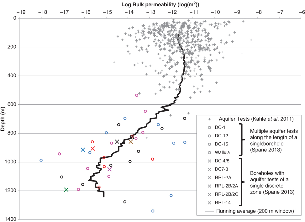
Fig. 13.4 Estimates of bulk horizontal permeability from Kahle et al. (2011) and Spane (2013). Using a 200 m window to compute a running average identifies a depth range of 600–900 m where permeability rapidly decreases. Above 600 m depth, average permeability is approximately constant. The deep data are sparse, but below 900 m depth, the rate of decrease in permeability apparently slows. Circles of the same color denote packer tests at different elevations within the same borehole. All other symbols represent single tests within a discrete borehole. (See color plate section for the color representation of this figure.)
The detailed Columbia River Basalt Group aquifer transmissivity estimates of Spane (2013) were also converted to estimated permeability (Fig. 13.4). First, estimated transmissivity was converted to bulk hydraulic conductivity by dividing by 30 m or the open length of the borehole, whichever was longer. Short open boreholes were assumed to test individual aquifers, so a typical lava flow thickness of 30 m was assumed to convert the aquifer test to a bulk permeability by using the layered system approximation (Fetter 1994, pp. 123–124). Long open borehole tests (>30 m) potentially intersected multiple aquifers and a representative length of confining unit. Temperature measured in these boreholes (Schroder & Strait 1987; McGrail et al. 2009; Spane et al. 2012) was used to correct viscosity and density, and permeability was computed and assigned to the middle of the test interval. Four boreholes have multiple packer tests vertically along the borehole length.
The permeability estimates exhibit considerable variability, but no persistent regional trends, so a running average value was computed using a 200 m window (line on Fig. 13.4). Available data define a substantial decline in permeability starting at a depth of about 600 m and slowing below 900 m. Similar rapid reductions in permeability with depth are documented for the volcanic rocks of the nearby Cascade Range by Swanberg et al. (1988), Blackwell (1994), Hulen & Lutz (1999), and Saar & Manga (2004). Because this rapid reduction in permeability has been suggested to correspond to hydrothermal alteration of volcanic rocks to pore-clogging clay minerals in the temperature range of 30–50 °C, the estimated aquifer-test temperatures were plotted against permeability (Fig. 13.5). The rapid reduction in aquifer-test permeability corresponds to a similar temperature range of 35–50 °C, suggesting that hydrothermal alteration may also cause the reduction in permeability with depth in the Columbia Plateau Regional Aquifer System.
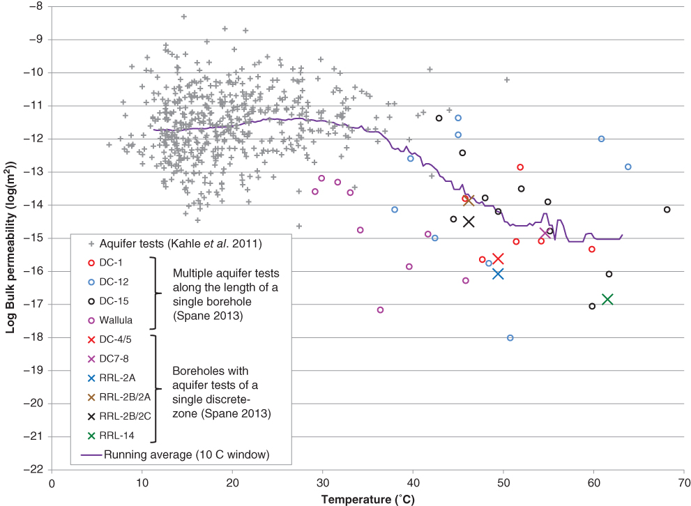
Fig. 13.5 Plot showing that permeability transitions rapidly in the temperature range 35–50 °C. For the Kahle data, temperatures were estimated from the nearest temperature log (Fig. 13.2). For the remaining aquifer tests, temperatures were estimated from temperature logs collected within the borehole during a battery of geophysical tests. (See color plate section for the color representation of this figure.)
Although there are no well-test data below 1400 m depth, permeability must be assigned to the full thickness of the Columbia River Basalt Group layers, which is almost 5000 m thick near the center of the Columbia Plateau Regional Aquifer System. Manning & Ingebritsen (1999) observed that for geologic materials in general, the rate of reduction in permeability is rapid near the land surface but slows with depth. Manning & Ingebritsen proposed a power-law fit to the data to define the permeability/depth relation. For the Cascade Range, Saar & Manga (2004) proposed altering the Manning & Ingebritsen relation by using piece-wise continuous exponential relations near the land surface to capture three distinct zones: an upper high-permeability zone, a middle zone of rapid reduction in permeability, and the deep Manning & Ingebritsen power-law relation.
For the SUTRA simulations of the Columbia Plateau Regional Aquifer System, three different permeability/depth relations were considered (Fig. 13.6): (i) Manning & Ingebritsen (hereafter called the “power-law depth relation”), (ii) Saar & Manga (hereafter called the “piece-wise-600 m depth relation”), and (iii) constant permeability with depth (hereafter called the “constant-permeability depth relation”). The original Manning & Ingebritsen power-law depth relation was shifted to the left by one order of magnitude to better fit the horizontal permeability data (in other words, permeability is 10 times less for the Columbia Plateau Regional Aquifer System), so that the curve passes through the running average of deep permeability observations. The power-law decay rate was unaltered. The piece-wise-600 m depth relation was fit to the horizontal permeability data such that above 900 m, the exponential relations are fit to the data, and below 900 m, the power-law depth relation is approximated.
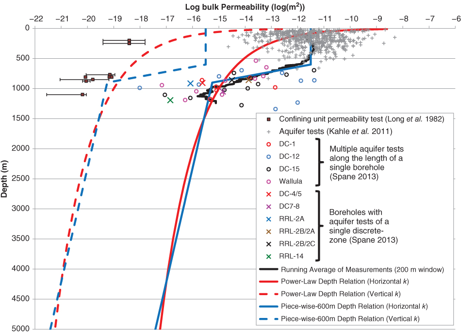
Fig. 13.6 Estimated permeability vs. depth relations for use in the SUTRA models. The solid lines are the maximum (subhorizontal) permeability, and the dashed line is minimum (subvertical) permeability. The red lines are the power-law depth relation. The blue lines are the piece-wise-600 m depth relation. The constant-permeability depth relation model is not shown, but has a log permeability of −11.55, indistinguishable from the shallow exponential model value of −11.5. (See color plate section for the color representation of this figure.)
Because the deep borehole tests are from a very limited areal extent, near a major fault zone, it is possible that they are not representative across the Columbia Plateau Regional Aquifer System. Consistent with recent regional modeling (Ely et al. 2014), the other end-member to consider is the constant-permeability depth relation. The permeability value used for the constant-permeability depth relation model was adjusted slightly to ensure a similar distribution of groundwater fluxes and shallow hydraulic heads between scenarios, as discussed in more detail later.
Consistent with previous regional groundwater flow simulations (Ely et al. 2014), bulk vertical permeability is assumed to be four orders of magnitude lower than horizontal permeability for each permeability–depth relation (Fig. 13.6). With increasing depth, the bulk vertical permeability should approach the permeability of individual flow interiors (Confining Unit Permeability Tests on Fig. 13.6), which are typically >4 orders of magnitude less than the aquifer-test data.
SUTRA simulations
Coupled groundwater and heat flow was simulated for two cross sections (Figs 13.2 and 13.7) using SUTRA (Voss & Provost 2002). The cross sections represent two typical groundwater flow paths from recharge areas to the Columbia River. Cross Section A–A′ represents the gently sloping Palouse Slope, which receives relatively little recharge and drains toward both the Snake and Columbia Rivers. Cross Section B–B′ represents the flow from one of the highest recharge areas, the Blue Mountains, toward the Columbia River. To the northwest of the section lines (Fig. 13.2), the dominant direction of geologic structure prevents accurate simulation of conditions using a 2D model. The two selected cross sections represent the range of conditions encountered in the remainder of the Columbia Plateau Regional Aquifer System.
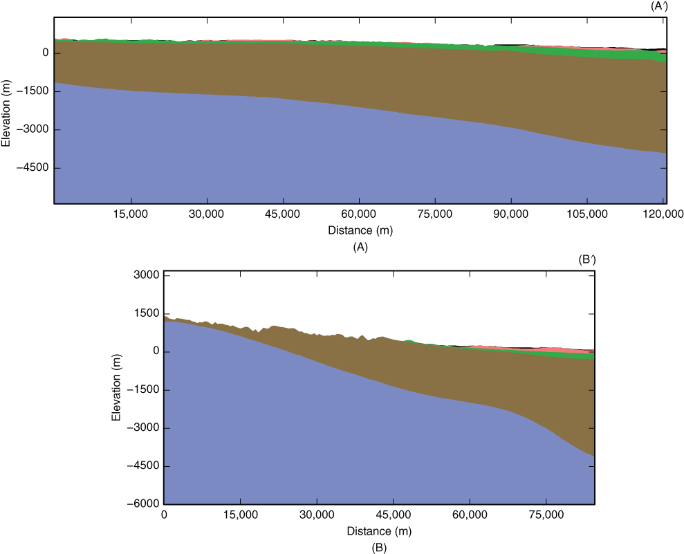
Fig. 13.7 Typical cross sections through the Columbia Plateau Regional Aquifer System (see Fig. 13.2). For both cross sections (units in m), the Columbia River is at the right-hand boundary, incised 250–300 m into the geologic units. (A) Cross section through the relatively gently dipping, low-recharge Palouse Slope. (B) Cross section from the crest of the higher recharge Blue Mountains through the Umatilla River basin. (Blue, pre-Miocene rocks; brown, Grande Ronde Basalts; green, Wanapum Basalts; red, Saddle Mountains Basalts; black, thin deposits of sedimentary overburden). (See color plate section for the color representation of this figure.)
Modifications to SUTRA
Version 2.2 of SUTRA was modified to improve the simulation capabilities over a wider range of temperatures (Alden Provost, U.S. Geological Survey, written communication, 2013). In general, water density and viscosity are functions of both pressure and temperature, though up to about 300 °C and 500 bars (about 5000 m of water pressure) the dependence on pressure is weak compared to the dependence on temperature (see Fig. 4.1 of Ingebritsen et al. 2006). SUTRA does not account for pressure dependence, but the nonlinear temperature-dependent water density and viscosity relations were improved to provide reasonably good fit up to approximately 300 °C (McKenzie &Voss 2013).
SUTRA was also altered to allow for spatially distributed thermal conductivity. SUTRA 2.2 only allows for a single homogeneous, possibly anisotropic thermal conductivity. Because the Columbia River Basalt Group has lower thermal conductivity than the underlying rocks (approximately 1.6 W m−1 per °C compared to approximately 2.5 W m−1 per °C), the thermal contrast can result in heat refraction at an inclined interface.
The last alteration to SUTRA 2.2 was to add a new type of boundary condition. For boundary conditions of the fluid, SUTRA 2.2 only allows for prescribed flux and prescribed pressure conditions. The new boundary condition is analogous to the MODFLOW drain boundary condition (McDonald & Harbaugh 1984), where water never flows into the model domain, but is allowed to leave the domain when pressure exceeds a fixed reference pressure. The rate of flow is proportional to the difference in these two pressures.
Model formulation, boundary conditions, and discretization
For the case where density and viscosity depend on temperature, the steady-state solution is achieved by running the simulation with steady boundary conditions for a very long time. Deming (1993) notes that the characteristic time of response for the fluid-flow problem is short compared to the heat-flow problem, so it is only necessary to estimate the characteristic timescale of response ( ) for heat flow:

with
where α is the thermal diffusivity, λbulk is the bulk thermal conductivity of the Columbia River Basalt Group (approximately 1.6 W m−1 per °C), ϵ is the estimated bulk porosity (estimated as 0.025), ρs is the density of the solid (rock) phase (approximately 3000 kg m−3), cs is the heat capacity of the solid (estimated as 840 J kg−1 per °C), ρw is the density of the fluid phase (estimated for this computation as 1000 kg m−3), and cw is the heat capacity of the fluid phase. The thickest part of the Columbia Plateau Regional Aquifer System is approximately 5 km and the simulated thickness below the Columbia Plateau Regional Aquifer System is 20 km, so the simulated domain is up to 25 km thick, providing an upper estimate for the characteristic length scale L. While the bulk thermal conductivity of the underlying rocks is higher, using the lower value for the Columbia River Basalt Group provides a conservative estimate of  of 2.52 × 10¹⁴ s (approximately 8 Ma). All variable density or variable viscosity simulations were run for a period greater than five times the characteristic timescale (1.26 × 10¹⁵ s) to ensure that the steady-state solution is approximated well.
A 2D regular mesh (Voss & Provost 2002) was used to represent each cross-sectional model, with approximately 30 m vertical discretization of the Columbia River Basalt Group on the right-hand side of the model (Fig. 13.8). Model cells thin from right to left, with the same number of vertical nodes representing the Columbia River Basalt Group across the domain. Horizontal node spacing is the same for all layers and is about 3000 m, except for the two vertical strings of nodes closest to the river, which are 300 m apart. The 20-km-thick ultralow-permeability unit below the Columbia Plateau Regional Aquifer System is simulated using 37 additional nodes (in the vertical direction) with a mesh that increases with depth from 30 m near the Columbia River Basalt Group units to a maximum of 1235 m at depth.
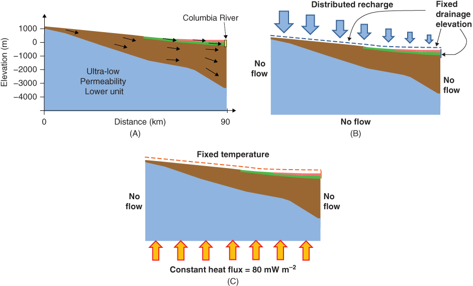
Fig. 13.8 Model formulation and boundary conditions: (A) hydrogeologic units with arrows showing that the preferential direction of permeability is rotated to align with the plane of basalt deposition (blue, pre-Miocene rocks; brown, Grande Ronde Basalts; green, Wanapum Basalts; red, Saddle Mountains Basalts); (B) hydrologic boundary conditions showing that recharge and discharge occur near the upper boundary and into the river on the right-hand side; (C) heat-flow boundary conditions showing the constant heat flux at the lower boundary and the prescribed temperature at land surface, with cooler temperatures in the uplands to the left. The thickness of the underlying ultralow-permeability unit was varied during model testing, with the final thickness being 20 km (figure not to scale for this unit). (See color plate section for the color representation of this figure.)
Within each hydrogeologic unit, the anisotropic permeability tensor is rotated so that the preferential flow direction is along the depositional horizon for each lava flow (Fig. 13.8A). The maximum rotation (6.5°) occurs at the contact between the Columbia River Basalt Group and the underlying unit near the right-hand model boundary. At the upper model boundary, dip parallels land surface. Permeability within the Columbia River Basalt Group is represented as a function of depth. Permeability in the ultralow-permeability region is set to 106 less than the overlying Columbia River Basalt Group permeability, ensuring that advective heat transport is negligible in the lower domain (Smith & Chapman 1983). Porosity is assumed to be 0.025 for all model cells. The isotropic bulk thermal conductivity of Columbia River Basalt Group units is set to 1.59 W m−1 per °C, and the underlying pre-Miocene rocks are set to 2.5 W m−1 per °C (typical values taken from Lachenbruch & Sass 1977).
The lower heat-flow boundary condition (Fig. 13.8C) is a constant uniform heat flux at a rate of 80 mW m−2. Upper-boundary and above-river-elevation nodes are set to the approximate annual average temperature for the period 1895–2007 extracted from the spatially distributed PRISM maps (PRISM Climate Group 2004). Except for the Columbia River, lateral boundaries are no-flow for fluid and fully insulated for heat.
All fluid flow ultimately enters and leaves the Columbia Plateau Regional Aquifer System at the land surface (Fig. 13.8B), and virtually every 3 km model cell contains a river or stream channel that can receive groundwater discharge (Ely et al. 2014). However, because the model is used to simulate the temperature of groundwater leaving the Columbia Plateau Regional Aquifer System, water cannot be allowed to flow out through the fixed-temperature boundary nodes. Instead, water is allowed to drain from the system at all nodes in the approximate depth range of 15–60 m, except at the Columbia River boundary. This depth range is consistent with the typical amount of stream incision shown schematically in the conceptual model (Fig. 13.3). At the Columbia River (right) boundary, boundary conditions transition at 30 m elevation (the river surface elevation), a depth of 150 m from the model upper boundary. Above 30 m elevation, in the depth range of 0–150 m, temperature is fixed on a vertical string of nodes on the right-hand boundary, and water is allowed to drain from the string of nodes of 300 m to the left in the depth range of 15–150 m. These conditions represent the incised “canyon” associated with the Columbia River. Below 30 m elevation, in the depth range of approximately 150–350 m, water is allowed to drain from the right-hand boundary nodes with a fixed pressure corresponding to 30 m of elevation. Extending the drain nodes as much as 200 m below the river elevation at this location is consistent with the 3D geometry of the Columbia River, which intersects the Grande Ronde unit at various locations along its length (controlled by faults, folds, and inclined beds).
Groundwater recharge from precipitation (Fig. 13.8B) enters the model into the same nodes where drainage is simulated (between 15 and 60 m depth) for all locations except the Columbia River, where no precipitation recharge is simulated. Temperature of recharge water is set to the same temperature as the fixed-temperature nodes. Recharge rates were estimated using a regression equation for the Columbia Plateau that relates average annual precipitation to recharge (Bauer & Vaccaro 1990). Annual average precipitation for the period 1895–2007 was estimated from the PRISM model (PRISM Climate Group 2004). There are no persistent trends in annual precipitation during this period though there are decadal scale variations corresponding to wet and dry periods.
Calibration
The remainder of this section and all figures pertain to the Blue Mountain–Umatilla cross section (Section B–B′ on Figs 13.2 and 13.7B), where groundwater flow is relatively vigorous. The Palouse cross section (Section A–A′ on Figs 13.2 and 13.7B) is considered only in “Discussion” Section.
Prior to examination of temperature simulation results, the groundwater simulation was “calibrated” for each of the permeability/depth relations. For the piece-wise-600 m depth relation, drain conductance was adjusted in two groups: all land surface drains and the Columbia River drains. These two parameters were adjusted such that the resulting hydraulic heads in the uplands near the crest of the Blue Mountains (left-hand model boundary) were near land surface elevation, hydraulic heads midslope are above land surface (confined conditions with upward gradient), and 38% of the total groundwater is simulated as exiting the system into the Columbia River boundary. These values are consistent with measured conditions.
The other two permeability/depth relations were calibrated to these same conditions, with the most important consideration being a similar distribution of groundwater discharge (which strongly influences advective transport of heat). Failure to incorporate hydrologic constraints can lead to erroneous conclusions regarding the importance of certain parameters. For example, applying the shallow permeability value from the piece-wise-600 m depth relation (Fig. 13.6) to the entire model thickness causes more than half of the total groundwater to exit the system at the Columbia River, transporting significantly more heat. The constant-permeability depth relation model was calibrated using a modest reduction in permeability (reduced from 10–11.5 to 10–11.55 m2) along with adjustment of drain conductance parameters. The power-law depth relation model was calibrated using only drain conductances.
Results
We first consider the effects of the piece-wise-600 m depth relation. Advective transport of heat by groundwater depresses temperatures near the higher recharge areas in the uplands and raises temperatures near the Columbia River. If only conduction of heat is considered (Fig. 13.9A), temperatures are slightly influenced by refraction as heat flows around the thicker parts of the relatively low-thermal-conductivity Columbia River Basalt Group units. When advective heat transport is added (Fig. 13.9B), cool groundwater recharged in the uplands cools much of the domain and raises temperatures below the Columbia River. The difference between the conduction-only simulation (Fig. 13.9A) and the combined groundwater and heat-flow simulation (Fig. 13.9B) shows that groundwater flow depresses temperatures by as much as 15 °C in some areas and elevates temperatures by up to 3 °C under the Columbia River (Fig. 13.9C).
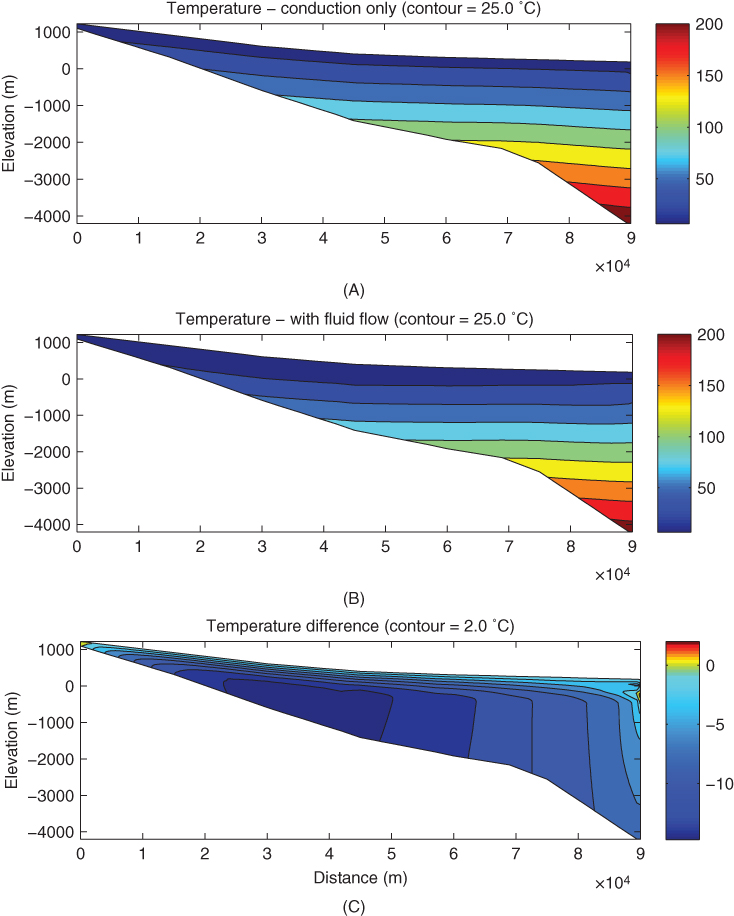
Fig. 13.9 Comparison of simulated temperatures for cross Section B–B′ (Umatilla) using the piece-wise-600 m depth relation. (A) shows the simulated subsurface temperature distribution assuming heat conduction only (no fluid flow). (B) shows the simulated temperature distribution for combined groundwater and heat flow. (C) shows the temperature difference between the two simulations; warmer colors show areas where temperatures are elevated by advective transport of heat, and cooler colors show areas where subsurface temperatures are lowered by heat advection. Plots are only colored in the part of the domain occupied by Columbia River Basalt Group units. (See color plate section for the color representation of this figure.)
The power-law depth relation is characterized by very high-permeability near land surface that decreases very rapidly with depth (Fig. 13.6). Because permeability is approximately 1000 times greater than either of the other permeability relations very near land surface, virtually all of the recharge moves along the thin skin of the system to discharge in rivers and streams. Below this very thin upper region, there is very little groundwater flow, and therefore little advective perturbation of the heat-flow field. As a result, the temperature distribution is almost indistinguishable from the conduction-only model (Fig. 13.9A).
The constant permeability/depth relation model has a very similar distribution of groundwater discharge, with discharge to the Columbia River within 0.5% of the 38% simulated using the piece-wise-600 m depth relation model. The constant-permeability depth relation allows for deeper penetration of groundwater flow along the cross section. A comparatively narrow range of acceptable combinations of permeability and drain conductance can be used to calibrate this model, all of which support the same general pattern of temperature seen in the piece-wise-600 m depth relation model (Fig. 13.9B), albeit with significantly amplified temperature perturbances relative to the heat-conduction-only model. The maximum depression of temperature (centered at approximately 3500 m on Fig. 13.9C) shifts right to approximately 5000 m and is about 20 °C lower. The constant-permeability depth relation model is approximately 35°C warmer than the piece-wise-600 m depth relation model at a depth of approximately 500–2000 m in a very narrow zone directly under the regional groundwater discharge location (right-hand side).
Local vertical conductive heat flow was estimated by computing the vertical temperature gradient between nodes and multiplying by the thermal conductivity. For the piece-wise-600 m depth relation, vertical heat-flow estimates are strongly affected within the higher permeability zone above 600 m, with deeper effects most notably below the Columbia River (Fig. 13.10A). To allow comparison with heat-flow measurements (estimated from thermal gradients measured in discrete intervals of boreholes), best linear fits to simulated profiles at different depth intervals were used to estimate heat flow (Fig. 13.10B). Vertical conductive heat flow is broadly reduced in the uplands and more locally increased near the Columbia River. Except below the Columbia River, simulated vertical conductive heat flow is approximately 80 mW m−2 at most depths below 600 m (Fig. 13.10B).
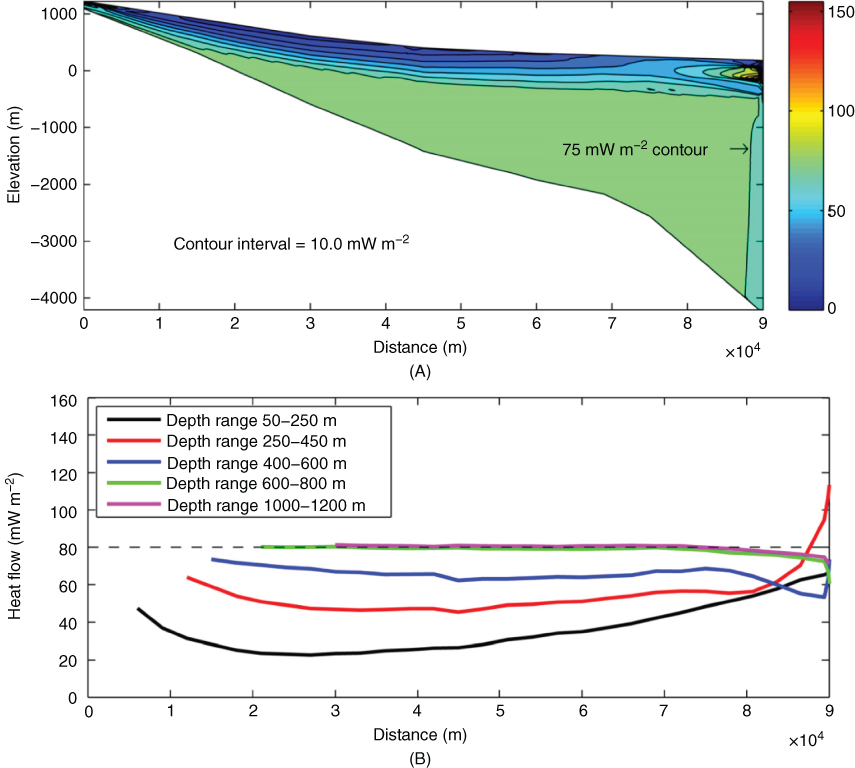
Fig. 13.10 Illustrations showing estimated vertical conductive heat flow for cross Section B–B′ (Umatilla) for the piece-wise-600 m depth relation: (A) local estimated vertical conductive heat flow and (B) estimated vertical heat flow for five depth ranges, computed as the bulk thermal conductivity times the representative gradient (slope of the best-fit line) of all temperatures in each depth range. Below approximately 600 m depth, heat flow is dominated by conduction. Plot A is only colored in the part of the domain occupied by Columbia River Basalt Group units. (See color plate section for the color representation of this figure.)
Because groundwater only flows in a thin skin near land surface for the power-law depth relation model, the entire model domain is very nearly constant at approximately 80 mW m−2. Heat flow is slightly higher to the left and slightly lower to the right, as heat is preferentially conducted around the thickest part of the low-thermal-conductivity Columbia River Basalt Group units, but when plotted on the same color scale as Figure 13.10A, virtually the entire domain falls within the 75–85 mW m−2 heat-flow contours.
For the constant-permeability depth relation, the rapid change in heat flow at a depth of approximately 600 m does not occur (Fig. 13.11). Simulated vertical conductive heat flow varies more smoothly with depth, asymptotically approaching 80 mW m−2. Otherwise, the heat-flow pattern is similar to Figure 13.10A though variability is amplified, with higher heat flow directly under the river, and lower heat flow in the shallow subsurface in the recharge areas.
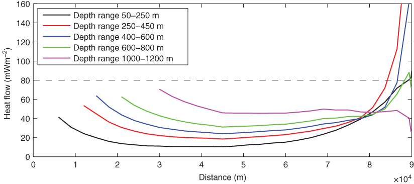
Fig. 13.11 Illustrations showing estimated vertical heat flow for cross Section B–B′ (Umatilla) for the constant-permeability depth relation. Estimated vertical heat flow for five depth ranges, computed as the bulk thermal conductivity times the representative gradient (slope of the best-fit line), of all temperatures in each depth range (compare with Fig. 13.10B). (See color plate section for the color representation of this figure.)
Despite the overall similarity in the groundwater discharge pattern at land surface, and groundwater discharge at the Columbia River being 0.5% lower, the heat removed advectively was significantly larger for the constant-permeability depth relation model. Groundwater carried 71.2% of the total heat exiting the system, compared to 58.2% of the heat exiting the system for the piece-wise-600 m depth relation model.
Comparison between model results and measured heat flow
In geophysical practice, vertical heat flow is determined from field measurements using a selected interval or intervals from a borehole temperature log. In order to compare estimates of vertical conductive heat flow from the simulations with field data, a best linear fit to the simulated vertical temperature profile at fixed depth intervals was used to produce transects of simulated vertical heat flow (Fig. 13.10B shows the estimates for the piece-wise-600 m depth relation).
Two depth intervals (50–250 and 250–450 m) were selected to represent the typical range of available heat-flow data (Fig. 13.2). To evaluate the role of the simulated rapid decline in permeability at 600–900 m depth, intervals of 400–600 and 600–800 m were also selected. Finally, a depth range below the permeability transition (1000–1200 m) was selected for comparison with the heat flow prescribed at the bottom boundary of the model.
For the piece-wise-600 m depth relation model, vertical heat flow below 600 m depth is very similar to the lower-boundary heat flow of 80 mW m−2 over most of the simulated cross section (Fig. 13.10B). Above 600 m depth, simulated conductive heat flow is significantly less than the deep conductive heat flow over much of the transect. The obvious exception is the high simulated heat flows near the Columbia River.
Heat-flow estimates from measurements (Fig. 13.12) are generally consistent with both the simulated values for the piece-wise-600 m depth relation model (Fig. 13.10B) and the constant-permeability depth relation model (Fig. 13.11). Several near-surface heat flow measurements near the Columbia River are markedly higher than 80 mW m−2, and upslope estimates are significantly lower. Spatial patterns in the measured data generally match the simulated profiles from <600 m depth (Figs 13.10B and 13.11), with lowest heat flows predicted midslope and higher heat flows near the crest of the Blue Mountains and the Columbia River. Because the power-law depth relation model predicts a constant value of 80 mW m−2 at all locations and depths, this model can be rejected. Because both the piece-wise-600 m and constant-permeability depth relations are deemed reasonable, the 2D cross-sectional model gives no indication of whether or not the shifted Manning and Ingebritsen relation is an appropriate representation of the deep (approximately >1 km) Columbia Plateau Regional Aquifer System. Future regional 3D modeling may provide some insight, but it is likely that additional deep thermal profile data would also be required to evaluate any deep permeability model.

Fig. 13.12 Heat-flow map with rivers; river line width is proportional to mean annual flow rate. Larger rivers are at the lowest elevations and receive water from long, regional groundwater flow paths. (See color plate section for the color representation of this figure.)
Given the same permeability distribution, the Palouse cross section (Section A–A on Figs 13.2 and 13.7A) exhibits less reduction in simulated vertical heat flow because the rates of groundwater recharge are lower and the groundwater flow system is less vigorous. Simulated heat flow under the Palouse was about 55 mW m−2 over most of the transect at a depth range of 50–250 m (analogous to Fig. 13.10B). At 250–450 m depth, simulated vertical heat flow was about 70 mW m−2, and below 600 m simulated heat flow was approximately 80 mW m−2, the lower-boundary value. Simulated heat flow near the Columbia River was elevated, but to a lesser extent than depicted in Figure 13.10.
Discussion
Simulation results using best estimates of hydrogeologic properties show that groundwater can remove sufficient heat to account for the apparent low-heat-flow anomaly without requiring anomalously low heat flow at the base of the Columbia River Basalt Group. Except for the power-law depth relation model, which resulted in most of the groundwater flowing through a very shallow zone, all simulation results show that, for a given depth, the highest temperatures will occur near major groundwater discharge zones. Previous heat-flow measurement has generally not focused on major groundwater discharge zones (Fig. 13.12), and most of the temperature measurements from wells are within depths perturbed by groundwater flow (Fig. 13.2). Deep boreholes far from regional groundwater discharge zones are likely the best estimators of regional heat flow.
Hansen et al. (1994) simulated the Columbia Plateau Regional Aquifer System using a range of hydraulic conductivities, with most of the system having bulk horizontal hydraulic conductivities in the range 3.5 × 10⁻⁶ to 3.5 × 10⁻⁵ m s−1 (1–10 ft d−1). These values correspond approximately to horizontal intrinsic permeabilities of 10–12.5 to 10–11.5 m2. The latter value was employed in this study (Fig. 13.6), and the former value may account for the role of geologic variability in restricting groundwater flow at a length scale longer than that represented by aquifer-test data. Lower permeability would require more water to drain in the uplands, which would result in less advective transport of heat. Our comparison of permeability/depth distributions assumed that the distribution of groundwater discharge was known, but in practice, groundwater discharge distribution is uncertain. An improved understanding of the distribution of groundwater discharge from the system would allow an improved understanding of both permeability and heat flow. Conversely, an improved understanding of the heat flow field can be used to constrain the groundwater flow rate.
Smith & Chapman (1983) showed that systems with much less anisotropy may exhibit much larger thermal effects. In our case, higher vertical permeability would allow water to flow more easily to the Columbia River, resulting in a larger thermal anomaly. A larger thermal anomaly would also result from increasing the depth of the permeability transition (600–900 m), with the end-member case being the constant-permeability depth relation model.
For most of the rivers receiving a large fraction of the deep regional groundwater flow, groundwater inflow is a relatively small fraction of total stream flow, so the thermal influence of groundwater is difficult to detect. The Umatilla cross-sectional model predicts that approximately 5.4 m3 s−1 of approximately 30 °C groundwater flows directly into the Columbia River (median annual flow approximately 5500 m3 s−1) along a 85-km reach. Although this simulated groundwater influx carries hundreds of megawatts of geothermal heat, the heat input will likely be thermally detectable only if focused monitoring is conducted at preferential groundwater discharge locations (subaqueous springs).
A limited amount of deep (>600 m) temperature data are available (Fig. 13.2), but these data are very near regional groundwater discharge zones and areas of significant structural complexity, indicating that heat flow in these areas may still have significant influence from groundwater flow.
Temperature measurements for 18 deep wells (>600 m) were compiled and, assuming a bulk thermal conductivity of 1.59 W m−1 per °C, estimated vertical heat flow below 600 m ranged from 55 to 71 mW m−2, with a median value of 63.5 mW m−2. Simulation results from the piece-wise-600 m depth relation model (Fig. 13.10) indicate that heat flow in discharge areas is on the order of 10% lower than the deep regional heat flow (Fig. 13.10). The constant-permeability depth relation model predicts larger reductions in conductive heat flow, so that either model supports an average vertical heat flow of ≥70 mW m−2, at or above the global average for tertiary tectonic provinces.
One confounding element in understanding the effects of permeability distribution is the hypothesis that a controlling factor is temperature, with an important transition at approximately 35–45 °C. In the uplands, these temperatures occur at greater depth, so our lowland-based estimate of the depth of transition (600–900 m) may be too shallow. Furthermore, elevated paleotemperatures (e.g., on the flanks of the Cascades) could have controlled hydrothermal alteration in some areas. Allowing a deeper transition to the low-permeability zone would result in behavior intermediate between the piece-wise-600 m and constant-permeability depth relation models (compare Figs 13.10B and 13.11). Preliminary exploratory simulations combining lower permeability values (similar to the lower permeabilities used in calibrated regional groundwater flow models [10–12.5 m2]) with deeper permeability transition depths (approximately 1000 m) yield simulated near-surface heat flow patterns that are also consistent with the existing heat flow estimates.
We have little information about the distribution of hydrothermal alteration minerals in the continental flood basalts of the Columbia Plateau Regional Aquifer System with respect to depth and temperature, although pore-filling alteration minerals (dominated by Fe-rich smectite clays, celadonite, zeolites, and silica) are commonly observed in flow tops and filling the joints and fractures of flow interiors (Reidel 1983; Horton 1991; Reidel et al. 2002; Zakharova et al. 2012). Detailed paragenetic studies of hydrothermal mineralization in basaltic rocks of the nearby Cascade Range and in the Hawaiian Islands do explicitly link hydrothermal alteration assemblages to depth and temperature. In Cascade Range, a significant decrease in permeability with depth in the range of approximately 200–1000 m is associated with temperatures in the range of 30–50 °C (e.g., Swanberg et al. 1988; Blackwell 1994; Hulen & Lutz 1999) and the appearance of a suite of pore-filling alteration minerals including clays and zeolites (e.g., Bargar 1988; Bargar & Keith 1999). At Kilauea Volcano, Hawaii, a significant reduction in permeability below 488 m is associated with temperatures of 30–60 °C and a suite of alteration minerals including calcite, Fe–Ti oxides, and Ca–Mg smectites (Keller et al. 1979).
For this study, heat generation within the model domain, either by decay of radionuclides (e.g., Deming 1993) or through viscous dissipation from fluid flow (Manga & Kirchner 2004), was neglected. Radiogenic heat production in basalts averages <0.4 μW m−3 (Vila et al. 2010), so the resulting difference in heat flow from the base to the surface of the Columbia River Basalt Group due to radiogenic sources will be <2 mW m−2 or approximately 2.5% of the background value. Manga & Kirchner (2004) estimate that the temperature of water increases through viscous dissipation by approximately 2.3 °C per 1000 m of elevation change from recharge to discharge location, indicating that the maximum heating of water for either cross-sectional model (Fig. 13.5) will be approximately 2 °C. This is potentially a non-negligible component of the temperature field (Fig. 13.9C) and the heat budget, but the general patterns of temperature and heat flow will be unaffected. The maximum error in estimated heat flow (Fig. 13.10A) resulting from neglecting this term is approximately 2% and occurs where the vertical temperature gradient is lowest (between 20 and 50 km; Fig. 13.9C).
Conclusions
Average heat flow at depth under the Columbia Plateau Regional Aquifer System is likely closer to the value of approximately 70–80 mW m−2 expected on the basis of its tectonic context than previous estimates from mapping of near-surface heat flow measurements (Williams & DeAngelo 2008, 2011) have indicated. Patterns and rates of groundwater flow computed using best-available estimates of hydrologic properties and boundary conditions can explain the apparent low-heat-flow anomaly. Near-surface heat flow is predicted to be relatively low in high-recharge upland areas and relatively high near major groundwater discharge locations (e.g., where deep aquifers intersect lowland rivers). Highest subsurface temperatures at a given depth are predicted to occur under the major rivers.
Compiled hydraulic test data from near the center of the Columbia Plateau Regional Aquifer System indicate that permeability decreases significantly in the depth range 600–900 m, corresponding approximately to a subsurface temperature range of 35–50 °C. Thus, in situ heat flow estimated below such depths will more reliably predict the deep, background heat flow.
The permeability decrease in the Columbia Plateau Regional Aquifer System occurs at temperatures similar to those associated with sharp reductions in permeability with depth in basalts of the adjacent Cascade Range and in the Hawaiian Islands, two localities where loss of permeability is known to be associated with hydrothermal alteration. Thus, we surmise that the permeability decrease at 600–900 m depth in the Columbia Plateau Regional Aquifer System also owes to hydrothermal alteration and, based on the similarity of pore-filling alteration minerals across these volcanic terrains, postulate that rapid permeability reductions with depth will likely occur in other continental flood basalt provinces.
The semiarid Columbia Plateau Regional Aquifer System provides a good example of modest groundwater flow rates significantly altering crustal heat flow. Because continental flood basalt provinces exhibit high degrees of lateral hydraulic connectivity over considerable distances (at least in the upper permeable zone), advective disturbances to crustal heat flow are expected in the active groundwater flow domain, with a return to predominantly conductive heat flow below the active groundwater system. Given similar thermal and hydrologic boundary conditions, temperatures would be affected to greater depths in systems with less extreme permeability anisotropy.
Acknowledgments
Dave Norman, Jeff Bowman, and Jessica Czajkowski (all from the Washington State Department of Natural Resources) provided new data to augment the USGS geothermal database. Alden Provost (USGS Reston) provided the new version of SUTRA for use in this study, altering the code to ensure that matrix singularities did not occur in the deep (heat conduction only) part of the domain. He was also a wonderful resource when considering how to best apply the new general head boundary conditions. Jonathan Haynes (USGS Oregon Water Science Center) provided geologic model GIS support and figure preparation. Many thanks to reviewers, Ingrid Stober, Ying Fan, and one anonymous reviewer, and editors Mark Person and Tom Gleeson, for the obvious care and many excellent comments and suggestions that resulted in significant improvement of the original manuscript. Funding for this project was provided by the US Department of Energy – Geothermal Technologies Program and the USGS Energy Resources Program.