
Every instrument that has been designed to be sensitive enough to detect weak light has always ended up discovering the same thing: light is made of particles.
—Richard Feynman1
PHYSICS IN 1945
The great physicists of the early twentieth century gave us relativity, gave us quantum mechanics, and revealed the structure of atoms and nuclei. Their successors were poised to carry on with their work when World War II intervened and the younger generation was instead put to work designing bombsights, sonar and radar detection, instrument flight, and, of course, the nuclear bomb. At the same time, mathematicians were breaking German and Japanese codes while chemists, geologists, and other physical scientists were doing their part in putting science to use in the war effort.
They all succeeded spectacularly so that by war's end the physical sciences and mathematics were viewed in a new light by the public and politicians alike. Soon biology joined in the spotlight as its contributions to medical science, spurred on by the new technologies developed during and after the war, began to have a growing impact on human health. Science was respected as never before—and as never since.
Our concern in this book is atomism, so let us review the status of the physics of matter as of 1945, when the Manhattan Project scientists could get back to doing what they really wanted to do with their time—basic research.
By that period, all of known matter could be built from protons, neutrons, and electrons. Light was composed of photons, so it seemed that all we needed in order to understand everything was four “elementary” particles. Unfortunately (or fortunately for physicist employment), these four particles weren't the only ones out there. In 1932, the same year that Chadwick discovered the neutron, Carl D. Anderson found the antielectron, or positron, whose existence had been predicted by Dirac in 1929. In 1936, Anderson and Seth Neddermeyer stumbled upon another particle in cosmic rays that best can be described as a heavy electron. We now call it the muon. It is 207 times more massive than the electron, but it is similar in every other respect, including having an antimatter partner comparable to the positron.
And this wasn't all. Beta-decay reactions led Pauli to propose in 1930 that a neutral particle with small or possibly zero mass was carrying off invisible energy. Enrico Fermi dubbed this hypothetical particle the neutrino, the “little neutral one.” Experimental confirmation of the neutrino did not occur, however, until 1956, and it was eventually discovered that three different types of neutrinos and their antiparticles existed.
Despite these empirical successes, and many more that were to occur rapidly after the war, no credible models describe how particles interacted with one another. Four fundamental forces could be identified:
- The gravitational force, which acts on all particles including, as Einstein showed, the photon.
- The electromagnetic force, which acts on all electrically charged particles plus the photon.
- The strong nuclear force, which acts on only protons and neutrons.
- The weak nuclear force, which acts on all particles except photons.
Although Einstein's general theory of relativity is not a quantum theory, it accounts for all observations involving gravity. What's more, gravitational effects are observable only when one of the bodies involved is very massive, such as Earth or the sun, and are negligible otherwise. And so, in 1945, quantum physicists decided to focus on electromagnetism—in particular, the interaction of photons and electrons.
MORE HYDROGEN SURPRISES
Recall from chapter 6 that the relativistic quantum theory developed by Paul Dirac in 1928 was able to successfully calculate the fine structure of the spectral lines of hydrogen. These were attributed to the interaction between the magnetic field produced by the electron in its orbit around the nucleus and the intrinsic magnetic field of the electron itself. Most importantly, Dirac's equation showed that the magnetic moment of the electron, a measure of the strength of the field, is twice what it should be if the electron were simply a classical spinning charged sphere, just as had been observed. Furthermore, the spin quantum number of the electron was ½, which made no sense if it were just the sum of the orbital angular momenta of particles inside the electron, which have integral quantum numbers. From all that was known at the time, and all that is known to date, the electron is a point particle with no substructure. Points don't spin. Quantum spin has no classical analogue.
According to the Dirac theory, the atomic states with n = 2 and l = 0 or 1 (see chapter 6) have the same energy, 3.4 eV. That is, they are “degenerate,” and they sure look that way in the optical region of the spectrum. In 1947, Willis Lamb and Robert Retherford at Columbia University measured the microwave radio emissions from hydrogen and discovered that these two hydrogen states were separated by 1,058 million cycles per second (mc, now called megahertz), a frequency corresponding to an energy of 4.3 millionths of an electron volt. This was named the Lamb shift.
At the same time at Columbia, Isidor Rabi (1898–1988) and his students John Nafe and Edward Nelson observed a second split in a spectral line. In this case, the 13.6 eV ground state of hydrogen (n = 1, l = 0) was observed to be split by 1,421.3 mc, or 5.8 millionths of an eV.
This so-called hyperfine splitting was perhaps less of a surprise than the Lamb shift and attributed to the interaction between the magnetic field of the electron and that of the proton nucleus. In 1934, Rabi and collaborators at Columbia had measured the magnetic moment of the proton and found a value larger than expected for a pure “Dirac particle” such as the electron. Using the theoretical Dirac value of the electron's magnetic moment and the measured Rabi value for the proton, a splitting of 1,416.90 ± 0.54 mc was calculated. While this was close, the discrepancy was nevertheless significant given the exquisite precision of the measurements involved.
The fact that the measured magnetic moment of the proton was not what it should have been for an elementary particle was the first evidence that the proton is not a point particle but that it has a substructure. Furthermore, the neutron, which has zero charge, has a nonzero magnetic moment showing that it, also, is not elementary. In fact, the neutron's magnetic moment is negative, as if it contained a negative charge circulating about a positive charge (like an atom!). Later, as we will see in the next chapter, the proton and neutron are composed of fractionally charged quarks.
QED
Just prior to World War II, Dirac and several of the other quantum pioneers had developed a relativistic quantum field theory based on his relativistic quantum mechanics. This turned out to be calculable only to a first-order approximation. When the physicists tried to move to the next order, they encountered infinities in their calculations.
In 1947, Hans Bethe performed a calculation of the Lamb shift in which he treated the atom nonrelativistically and absorbed the infinities into the mass and charge of the electron, a process called renormalization. He obtained 1,040 mc, in good (if not perfect) agreement with the measured 1,062 mc.2
Following up on Bethe's intuition, a fully relativistic theory of how photons and electrons interact, renormalizable to all orders of approximation, was developed independently by Julian Schwinger3 and Richard Feynman4 in the United States and by Sin-Itiro Tomonaga5 working in war-ravaged Japan. The theory was dubbed quantum electrodynamics or QED.6 In 1949, Freeman Dyson, a Brit working at Princeton, showed that the three formulations were equivalent.7
In the spring of 1948, Feynman attended an invitation-only meeting at the Pocono Manor Inn in rural Pennsylvania. There he introduced a simple line drawing, now called a Feynman diagram, which would prove to be an invaluable tool in particle physics.8
The Feynman diagram was originally motivated by the need to keep track of various terms in QED calculations. Although Schwinger and Tomonaga did not use them, Feynman diagrams are very intuitive visual models of fundamental interactions that supplement a cookbook set of rules for calculating interaction probabilities. While many physicists view them as just calculational tools, others, like myself, look at them as bearing some relation to what is actually going on in nature.9
The first-order interaction of two electrons is illustrated in figure 9.1. One of the electrons (solid lines) emits a photon (dashed line), which carries energy and momentum to the other electron.
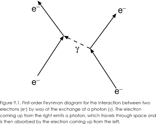
The lines in the diagram can be thought of as roughly representing the paths of particles in a two-dimensional space-time picture, with a space-axis to the right and a time axis up. Or, you can think of the arrows as representing momentum vectors. In neither case is this visual aid drawn to scale.
The notion that particles interact by means of exchanging other particles was not original with Feynman. Hans Bethe and Enrico Fermi had already proposed the idea of photon exchange in 1932. And in 1942, Ernst Stückelberg had used space-time diagrams similar to Feynman's to describe electron-positron pair production and annihilation.10 In any case, with Feynman diagrams and the rules for their use, we had a fully relativistic prescription for calculating the probability to higher orders of approximation.
If an electron is in an atom or in the presence of some external field, we can view the first-order interaction as in figure 9.2 (a), where the source of the incoming photon, not shown, is either the electric field or the magnetic field of the nucleus. To first order, the field emits a single photon. Feynman diagrams for second-order interactions are shown in figure 9.2 (b), (c), and (d). These provide the main contribution to the anomalous magnetic moment of the electron that deviates from the Dirac value. They're not as complicated as they look at a first glance. Just follow the particle lines from bottom to top and you can see the sequence of interactions.

Figure 9.2 (b), in which a photon converts to an electron-positron pair, which then converts back to a photon, is an example of vacuum polarization. During the time that pair is present, an electric dipole (pair of positive and negative charges) that can affect the path of the electron exists in otherwise empty space. This is the primary source of the Lamb shift, where, we can think crudely, the electron has different orbits for l = 0 and l = 1, so the two states are affected differently by the polarized vacuum.
We can also see from this discussion why physicists talk about the vacuum never being empty of particles. Pairs of particles can flit in and out of existence in what are called quantum fluctuations. Isolated pairs have no effect in quantum field theory, but these fluctuations are believed to couple to gravity as a cosmological constant. This is the notorious cosmological-constant problem, which will be discussed in chapter 12.
A common misunderstanding, even among many physicists, is that momentum and energy conservation are violated at the “vertices” of a Feynman diagram where a particle may split into two particles. This is usually explained as being allowed by the uncertainty principle. Actually, this is wrong. Energy and momentum are conserved everyplace in the diagram. The so-called virtual particles represented by internal lines that do not connect to the outside world may have imaginary mass, that is, negative mass squared. Recall that in units where c = 1, the mass m of a particle of energy E and momentum p is given by m2 = E2 – p2. This can be negative or positive. Imaginary mass presents no problem because the masses of virtual particles are never measured. And recall that I have defined matter as anything having energy and momentum, with no restriction on the sign of the mass squared.
In 1948, Feynman showed that an antiparticle going one direction in time is empirically indistinguishable from the corresponding particle going backward in time.11 The idea also had been proposed by Stückelberg in 1942.12 So, in all the diagrams we can draw, we can always reverse the arrow and change an electron to a positron. In the case of the photon, you are also free to reverse its arrow, but it is its own antiparticle, so there is no difference.
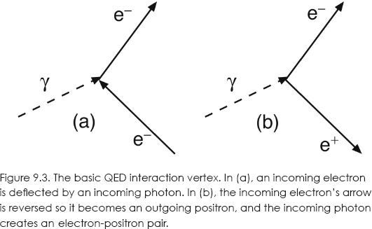
We see that many different diagrams can be drawn. However, note that they all have the same basic reaction in which two electrons interact with a photon at a point called a vertex. As shown in figure 9.3 (a), we can view it as an electron being scattered by a photon, or in figure 9.3 (b), as an incoming photon becoming an electron-positron pair. Reverse other lines and you will have other interpretations that are all experimentally indistinguishable.
In 1948, using his own highly sophisticated mathematical techniques, not based on Feynman diagrams (and so incomprehensible except to a select few), Schwinger calculated the electron magnetic moment by taking into account the second-order corrections. He obtained a value that was greater than the Dirac value by a fractional amount of 0.00118, in good agreement with experiment. Since then, QED calculations for the electron magnetic moment up to fourth order agree with the most precise measurements to ten significant figures.
Schwinger also obtained 1,040 mc for the Lamb shift, the same value calculated by Bethe. The current QED calculation, including higher orders, is 1,058 mc, which is in exact agreement with the current value of 1,057.864 mc. Since this original work, quantum electrodynamics has been tested to great precision without failure. QED may be the most precise theory in all of science.
FIELDS AND PARTICLES
The extraordinary success of quantum electrodynamics suggests that relativistic quantum field theory is telling us something about the nature of reality. But what exactly is it telling us? To explore that question, let us avoid the complications of interacting particles and consider an electromagnetic field all by itself.
Suppose we have an array of harmonic oscillators, for example, simple pendulums, each with a different natural frequency f. An electromagnetic field is mathematically equivalent to such an array, where each oscillator has unit mass and corresponds to one “radiation mode” of the field.13
In quantum mechanics, a harmonic oscillator of frequency f has a series of ladderlike, equally spaced energy levels separated by energy hf, where h is Planck's constant. Because of the uncertainty principle, an oscillator can never be at rest and the lowest energy level is ½hf. This is called the zero-point energy.
It follows, then, that the energy of an electromagnetic field is quantized in steps of hf, as proposed by Planck. When a transition occurs from one energy level to the next one below, a quantum of energy hf is emitted that we interpret as a photon of that energy. Thus, the field can be thought of as containing a certain number of photons, each of energy hf. Starting at the bottom of the ladder, the zero-point energy state has zero photons. The next rung of the ladder has one photon; the next, two; and so on. The total energy of each radiation mode of the field is then the zero-point energy plus the sum of the energies of the photons in the field: ½hf + hf + 2hf + 3 hf +….
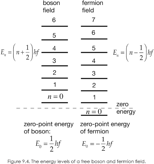
Now, this picture can be shown to apply to all bosons (integer spin particles). In the case of fermions (half-integer spin particles), we have the same ladder except the zero-point energy is –½hf. (Negative energies are allowed in relativity.)
In short, a field-particle unity exists such that for every quantum field, there is an associated particle that is the quantum of the field. In the 1970s, physicists developed the standard model of particles and forces based on relativistic quantum field theory in which each elementary particle is the quantum of a quantum field.