Figure 6.1. Illustration showing water waves propagating away from the point of impact of a pebble.
Thus far, static methods have been used to characterize the shallow subsurface environment. The term 'static' implies that the quantity of interest does not change over time. Waves are 'dynamic' meaning that they are quantities that vary over time. In the static methods considered (gravity and magnetometry), characteristics of buried objects are inferred from spatial changes in the gravitational acceleration and magnetic field. In particular, feature depth can only be estimated indirectly from these spatial variations (Sects. 4.12 and 2.12.1). Dynamic methods are complicated by the need to record and interpret temporal variations as well as spatial variations. With this complication comes additional benefits in feature characterization, and perhaps the most important of these benefits is the direct determination of object depth. This chapter will introduce some basic concepts of waves that are necessary to the understanding of the use of waves in geophysics, In many respects, waves are a more difficult topic than the previously presented static methods; however, waves are more intuitive since waves are exploited in daily life. The human body cannot directly 'sense' magnetic fields and, while the body can 'sense' gravity, it is not sufficiently sensitive to provide any experience as to the 'feel' of changing gravitational acceleration. Conversely, there is a great deal of direct experience in sensing and exploiting waves. Both light and sound are wave-based phenomena and these types of waves are sensed by sight and hearing, respectively, and interpreted by the brain. Thus, there are instinctive skills used in exploiting waves that can be directly called upon for use in the geophysical exploitation of waves.
In geophysics, the most important characteristic of waves is that they propagate. Propagation means traveling with a certain speed and, because waves propagate, it is possible to directly measure distances. For example, consider driving a car at a constant speed between two cities without stopping. By knowing the speed and measuring the time required to complete the drive, it is possible to determine the distance between the two cities. This introduces the most fundamental relationship used in the analysis of waves. This is, that distance is equal to speed multiplied by travel time. Denoting speed by c, time by t, and distance by l, and assuming for illustration purposes that the driving speed is 30 kilometers per hour and that the trip requires three hours, the distance between the two cities is simply
l = c X t = 90 km.
Although traveling in a car does not involve waves, this simple example is quite similar to a wave-based measurement. To illustrate this, consider throwing a pebble into a pool of water (Fig. 6.1).
Figure 6.1. Illustration showing water waves propagating away from the point of impact of a pebble.
As is well known and illustrated here, the impact of the pebble on the water surface produces waves that appear as circular ripples. To determine the distance from the point where the pebble hits the water it is sufficient, knowing the speed of the wave, to measure the time required for the wave to reach a particular point and then compute the distance using l = c X t.
Perhaps a better example is a digital tape measure. This device emits a short burst of high frequency (above audible) sound. This sound travels with a characteristic wave speed (about 340 meters per second in air), bounces off an object and returns to the instrument where the returning wave is detected. The use of a digital tape measure to determine the distance to a wall is shown in Fig. 6.2. The main components of the digital tape measure are elements (transducers) to generate and detect sound, and a clock.
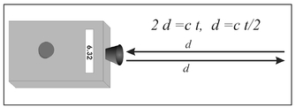
Figure 6.2. Illustration of the use of a digital tape measure to determine the distance to a wall.
The clock starts 'ticking' at the time the sound is generated and the device 'counts' clock ticks until a returning sound is detected. The total distance / this sound wave travels is l = c X t. However, the sound must travel from the device to the wall and then back. Therefore, the distance to wall d is one-half of the measured distance or
The fact that waves travel makes them dynamic rather than static because the situation is changing over time. While this may not be immediately obvious in the examples presented thus far, it certainly is the case. To understand this, reconsider the problem of driving between the two cities. Here, like the digital tape measure, you are somehow continuously counting clock ticks and, for most of the drive, simply noting that you have not arrived yet. This continues until you actually do arrive, at which time you note the arrival time and discontinue the measurement. Consider making the same drive but, along the way, you wanted to determine the distance between intermediate cities. The measurement procedure is the same, but you must record more information.
The examples given above serve to illustrate the use of time-based measurements. The dynamic nature of waves is somewhat more complicated. Consider now wind-driven waves approaching a beach (Fig. 6.3).1
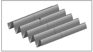
Figure 6.3. Illustration of a train of water waves approaching a beach.
Here, there is a train of wave crests and troughs parallel to a beach. If a photograph is taken of waves approaching a beach, it would appear similar to Fig. 6.3 and measuring the water surface elevation with respect to an undisturbed water surface level along a direction perpendicular to the beach (along the black line drawn on Fig. 6.3) there would be a series of alternating crests and troughs at a fixed spacing between adjacent crests or troughs (6.4). Occupying a fixed point in the water (the black circle shown on Fig. 6.3) and making measurements of water elevations over time, a similar pattern of alternating crests and troughs (Fig. 6.5) would be recorded.
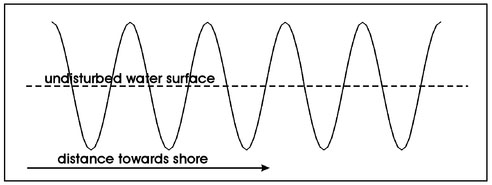
Figure 6.4. Illustration of the spatial variations in water waves with measurement position. The vertical axis is displacement of the water surface.
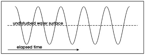
Figure 6.5. Illustration of the temporal variations in water waves with measurement time. The vertical axis is displacement of the water surface.
From Figs. 6.4 and 6.5, it is clear that propagating waves change over both time and space. Taking a 'snapshot' of water waves (Fig. 6.3) and measuring surface elevation as a function of distance from the shore and then taking another snapshot a very short time later, there would be a similar pattern of crests and troughs. But a comparison of the relative positions of crests and troughs would reveal a slight shift between the two snapshots. For example, where crests occur in one snapshot, troughs could occur in the other. This shift in pattern can be predicted from the fundamental relationship and, for a wave traveling with a speed c, the distance the pattern has shifted is c multiplied by the time interval between the two snapshots.
Waves are characterized by changes in both space and time and temporal changes are related to changes with respect to spatial location. Some important parameters that characterize a wave can now be introduced. Figure 6.4 shows the change in surface elevation of a water wave with a shoreward measurement position. In this figure, the distance between adjacent crests (or adjacent troughs) is known as the wavelength of the wave and the vertical distance from the crest (or trough) to the undisturbed water surface is the amplitude of the wave. These parameters are identified in Fig. 6.6a. A similar pattern of crests and troughs appears when making measurements of water surface elevation over time at a fixed location (Fig. 6.5).
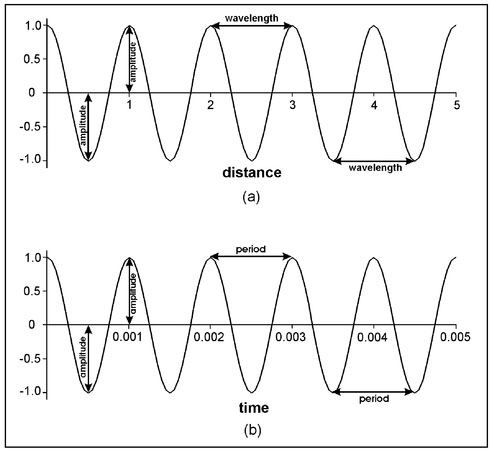
Figure 6.6. Illustration defining the wavelength, period, and amplitude of water waves. The vertical axes are displacement of the water surface.
The time elapsed between adjacent crests (or adjacent troughs) is known as the period of the wave. Again, the vertical distance between a crest (or trough) and the undisturbed water surface is the amplitude of the wave. These parameters are identified in Fig. 6.6b. The standard abbreviations for wavelengths and periods of waves are
γ—the lower case Greek letter lambda, for wavelength and
τ-the lower case Greek letter tau, for period.
There is no standard abbreviation for wave amplitude.
For waves, propagation time and propagation distance are related through the wave speed c. Since the wavelength is essentially a measure of distance and the period is a measure of time, it might be surmised that wavelength and period are also related through the wave speed. This is indeed the case and the relationship between wavelength and period is the same as the relationship between distance and time,
γ= c X τ
Another wave parameter and one that is related to the wave period, τ, is the frequeny'. Frequency is usually denoted by f and it is related to the wave period by
Common electrical current as used in a home is called alternating current (AC) because the polarity of the current alternates between positive and negative. The change in polarity is like wave crests and troughs so that AC current is wave-like. In the United States, this current changes polarity at a rate of sixty cycles per second where one cycle is a change in polarity from positive to negative and then back to positive. Thus, the frequency of AC current is sixty cycles per second and its period, from the equation above, is 1/f = 1/60 = 0.017 seconds. The common unit of frequency is Hertz (abbreviated as Hz) where 1 Hz = 1 cycle per second.
It is clear from the above relationships that a wave of high frequency has a short period and, for a given wave speed, a high frequency wave is characterized by a short wavelength.
For the wave shown in Fig. 6.6, the amplitude is 1 m, the wavelength, μ, is 1 m, and the period is 0.001 seconds. For this period, the frequency, f, is 1000 Hz. Using the above-cited relationship between wave speed, wavelength and period, the wave speed is c = γ/τ = 1000 m per second. The same result can be obtained using the definition of frequency or c= αf.
A final wave parameter is the phase normally denoted by φ, the Greek letter phi. This is a relative quantity that describes the relationship between waves having the same wavelength or period. The phase is the extent to which one wave form must be shifted so that all the peaks and troughs are aligned. Figure 6.7 shows two waveforms having the same wavelength or period but different amplitudes. The first peak of the wave shown as a solid line occurs at zero while the first peak of the wave displayed as the dashed line occurs at two. By sliding the dashed wave backwards a distance of two units, the peaks and troughs of the waves will coincide. Thus, the relative phase between these two waves is two. It doesn't matter if these plots represent the change with distance or time. The only distinction is the units assigned to the phase, for example, seconds for temporal changes or meters for spatial variations. The phase is independent of the amplitude of the waves.
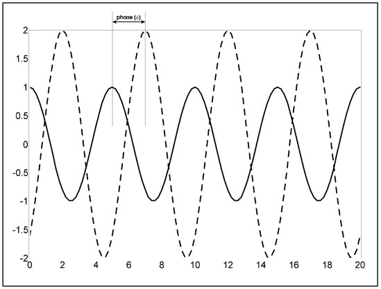
Figure 6.7. Illustration of the relative phase between to waves of equal wavelength or period.
There are many types of waves and there can be a number of distinguishing characteristics such as the form of energy used to generate them, how they propagate, the medium in which they propagate, and so on. Here, various general categories of distinguishing characteristics of waves are explored. It is important to note, however, that no single characteristic completely defines a wave. As will be demonstrated here, waves may be mechanical and transverse, mechanical and longitudinal, electromagnetic and decaying, and so on.
The differentiation between transverse and longitudinal waves is a distinction between the direction of oscillation and the direction of propagation. A transverse wave is a wave where the direction of oscillation is perpendicular (transverse) to the direction of propagation. For water waves, the water surface oscillates up and down while the waves propagate horizontally. Therefore, water waves are transverse waves. Although this can never happen, consider a water wave that propagates towards the shore with the water surface oscillating horizontally but parallel to shore. Since these oscillations are perpendicular to the direction of wave propagation, this is also a transverse wave. Thus, another parameter is needed to characterize a transverse wave and this is the direction of oscillation. The direction of oscillation is referred to as the polarization of the wave. The waves depicted in Fig. 6.1 and Figs. 6.3 to 6.7 are vertically polarized transverse waves.
Because water waves can be seen, there is an intuitive understanding of transverse waves. Waves can also oscillate in the direction of propagation and these waves are known as longitudinal waves. Sound waves are longitudinal waves. Although sound waves can obviously be heard, they cannot be seen. For this reason, longitudinal waves are not as intuitive as transverse waves. Figure 6.8 presents an experimental sequence to illustrate the propagation of a longitudinal wave.
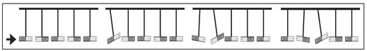
Figure 6.8. An illustration using magnetic repulsion to demonstrate the propagation of a longitudinal wave.
Shown here is a row of equally spaced magnets suspended from a wire so that they can swing freely. The magnets are oriented such that the pole of any magnet is facing the same pole of adjacent magnets. Except for the end magnets, each magnet hangs vertically because the repulsive force of an adjacent magnet is balanced by an equal but opposite repulsive force exerted by the magnet on the other side. By starting the magnet on one end swinging, a 'chain reaction' is started that creates a longitudinal wave. With the first swing, the first magnet moves closer to the second magnet, thereby increasing their mutual repulsive force. The force of the second magnet on the first forces it to swing back towards its original position while the force of the first magnet on the second magnet causes the second magnet to swing to the right. With this swing to the right, the second magnet becomes closer to the third magnet and the above-described sequence of events is repeated. This sequence 'propagates' along the entire line of magnets as a wave. The movement of each magnet is along the same direction as the propagation of the wave and, hence, this is a longitudinal wave.
A similar situation occurs in sound waves. While the forces acting in the magnetic example of Fig. 6.8 are magnetic attraction and repulsion, the forces acting to produce sound waves are compression and expansion. Figure 6.9 is an illustration, similar to Fig. 6.8, of how sound waves propagate.
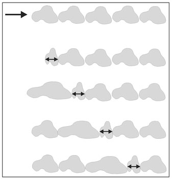
Figure 6.9. An experimental sequence illustrating how the forces of compression and expansion produce sound (longitudinal) waves.
This figure shows a number of small volumes of a gas. These parcels are referred to as control volumes. The wave is initiated by pressing laterally on the first control volume and then releasing. This control volume is compressed, squeezed between the applied force and the second control volume. This is analogous to squeezing a balloon. The first control volume tries to expand to return to its original shape and, in doing so, it 'overshoots' its original volume (it temporarily becomes larger than its original size) and thereby squeezes the second control volume. The second volume is compressed and expands squeezing the third control volume. This sequence propagates along the row of control volumes and, since the direction of compression and expansion is the same as the direction of propagation, this is a longitudinal wave.
Thus far, waves have been characterized by their wavelength, period or frequency, phase, and direction of oscillation relative to propagation. Another means by which waves can be characterized is according to what happens to their amplitudes as they propagate.
In general, waves diminish in amplitude as they propagate away from the point of generation. This is quite obvious since it is well known that sound, light, and radio waves do not travel forever. The signal received by a radio gets weaker as its distance from the broadcast point increases. Figure 6.10a displays the pattern of waves produced by dropping a pebble into water. The wave oscillations along a direction radiate outward from the point of impact (the solid line on Fig. 6.10a) as plotted in Fig. 6.10b. This plot is similar to the plot of water wave amplitude as a function of distance shown in 6.4 except that here the amplitude of the wave decreases with distance.
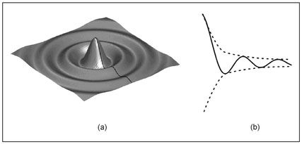
Figure 6.10. Illustration showing (a) the line along which (b) the decay of water wave amplitude with distance is plotted.
The dashed lines drawn on this figure show the decrease in amplitude with distance. These lines are referred to as the envelope of the wave.
There are a number of mechanisms that cause wave amplitudes to diminish with propagation distance. The first to be considered is geometric spreading, in which a fixed total amount of energy spreads out over an ever-increasing area or volume. Returning to the example of ripples created by dropping a pebble into the water (Fig. 6.1), it can be expected that, in the absence of any mechanism for energy loss such as friction, the amplitude of the wave will decrease with propagation distance away from the point of pebble impact in a manner similar to that shown if Fig. 6.10b. It is also observed in Fig. 6.10a that wave crests appear as concentric circles about the point where the pebble strikes the water. Since there is no energy lost from this wave as it propagates, the energy in every crest must be the same. The crest further out has a larger perimeter as well as a smaller amplitude and thus the energy must somehow be 'diluted.' This situation is illustrated in Fig. 6.11 which shows two concentric circles representing wave crests a distance r1 and r2 away from the point of impact.
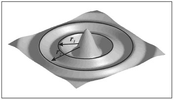
Figure 6.11. Illustration of the geometric spreading of ripples on the water surface.
As noted above, the energy in each crest is the same. However, the energy density, defined by
where it is recalled that π about 3.14. Since r1 is less than r2 the energy density is greater at a distance r1 than it is at r2. An analogy to geometric spreading is the stretching of a rubber band. Like the energy in the water wave considered above, the amount of rubber in a rubber band does not change as the rubber band is stretched. However, the more the rubber band is stretched, the thinner it becomes. The thickness of the rubber band is inversely proportional to its perimeter.
Water waves are special in that they are constrained to travel over the surface of the water rather than in a volume. The waves considered in geophysics all propagate through a volume (in three-dimensions) so that it is appropriate to define energy density using a surface area (rather than a perimeter). Making this generalization, it is clear that geometric spreading causes a decrease in energy density proportional to the distance squared. Recalling that a gravity anomaly decreases as the square of the distance away, it is noted that geometric spreading also behaves like a monopole. A wave source produced by a symmetric, localized disturbance is known as a point source and the geometric spreading produced by point sources behaves like monopoles. In fact, measuring waves produced by a point source over some flat surface and creating a contour plot of wave energy density over this surface, it would look remarkably like the contour plot for the gravity anomaly caused by the buried sphere shown in Fig. 2.25. Thus, there is some commonality between waves and static energy sources such as gravity. It is important to note that wave energy is proportional to the square of wave amplitude. This means that for waves generated by a point source, the amplitude decreases with distance while the energy density decreases with the square of the distance.
Waves that travel without loss of energy (although there could be a loss in amplitude through geometric spreading) are referred to as propagating waves. Waves that lose energy as they propagate are referred to as decaying waves. One obvious source of energy loss is friction. Figure 6.12 illustrates a wave form produced by a point source where there is loss of amplitude through geometric spreading (solid line). If, in addition to geometric spreading, there is a reduction in amplitude due to energy loss, this energy loss will cause a loss of amplitude in excess of that resulting from geometric spreading. The dashed line on Fig. 6.12 is a decaying wave and by comparing the two wave forms shown here it is clear that there is a loss of amplitude beyond that associated with geometric spreading.
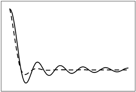
Figure 6.12. Plot of amplitude versus propagation distance from a point source for a loss of amplitude from geometric spreading (solid line) and additional amplitude loss caused by energy loss (dashed line).
As illustrated by the envelope (Fig. 6.10b), there is some characteristic rate of amplitude loss with distance. This amplitude loss can be caused by geometric spreading, decay, or both. This rate of loss in amplitude could be scaled with the wavelength of the wave and thereby defining a loss in amplitude per wavelength rather than the loss of amplitude over some arbitrary distance. If the loss in amplitude of a wave is taken to be independent of its wavelength, the sequence of situations such as depicted in Fig. 6.13 might be encountered. Here, the amplitude loss as a function of distance from the source varies for the three different wavelengths.
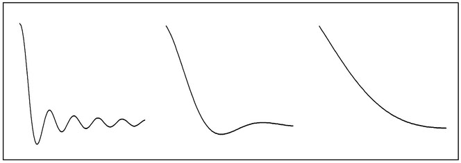
Figure 6.13. Illustration of wave amplitude, as a function of distance from the source, for three wavelengths.
The plot on the left is for a particular wavelength and the center and right plots are for successively longer wavelengths. Comparing the left and center plots, it is clear that the longer wavelength experiences fewer oscillations for a given loss in amplitude than the shorter wavelength. The wavelength could be made so large (the right plot) that the wave amplitude has decreased to a value too small to be measured before it has experienced even a hint of an oscillatory pattern. Waves of this type are referred to as evanescent waves. While evanescent waves do occur and can be exploited in geophysics, such an exploitation is far beyond the scope of this book. The purpose for their introduction is to illustrate a point. Consider a wave generated by a point source and experiencing a loss of amplitude associated with geometric spreading. The energy density will decrease with distance like a monopole. If the wavelength of this wave is infinitely large, there will be no oscillations, only a decay with the square of the measurement distance. This is exactly what was encountered in the static methods. Thus, static fields such as gravity and magnetic fields, can be considered as waves with infinitely long wavelengths.
Geometric spreading was introduced as a loss of amplitude without any energy loss. Another way to view geometric spreading is as a redistribution of amplitude or energy. As the wave from a point source propagates, its amplitude diminishes (Fig. 6.11). This amplitude and the associated energy is distributed over progressively larger circles. Wave amplitude can also be redistributed when a wave encounters an object. In this case, the redistribution is referred to as scattering.
To illustrate the mechanisms of scattering, first consider only a single crest from among the many parallel crests and troughs associated with a water wave propagating towards a beach (Fig. 6.3). This crest, now referred to as the incident wave, is approaching a vertical circular cylinder in the water (Fig. 6.14a). When the incident wave reaches the cylinder (Fig. 6.14b), a minute portion of the incident wave energy is redistributed as a result of its interaction with the cylinder. The effect of the interaction of the incident wave with the cylinder is that the cylinder radiates as if it is a point source (Fig. 6.1). This is illustrated in Fig. 6.14c as a single circular crest and this is referred to as the scattered wave. Because only a small amount of energy is converted from incident to scattered wave, the amplitude of the scattered wave is relatively small.
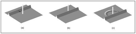
Figure 6.14. Illustration of the scattering of a single wave crest from a vertical cylinder. At an early time, (a) the incident wave is approaching the cylinder and (b) when this crest reaches the cylinder, a scattered wave is created. As the incident crest passes the cylinder, (c) the cylinder radiates as if it were a point source. The arrow indicates the direction of propagation of the incident wave.
It can be hypothesized that the nature of the scattered wave will depend on the size and shape of the scattering object. As an example consider the wave crest incident on a wall rather than a cylinder. It is likely that there will be area behind this wall where there will be no scattered wave (Fig. 6.15).
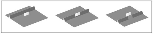
Figure 6.15. Time sequence illustrating the interaction of a single wave crest with a wall.
If a closely spaced row of cylinders (Fig. 6.16) is considered, rather than a single scattering object, it is expected that the nature of the scattering would qualitatively be somewhere between that from a single cylinder and a wall. This argument suggests that scattering can depend on the size, shape and spacing of objects that are exposed to a wave.
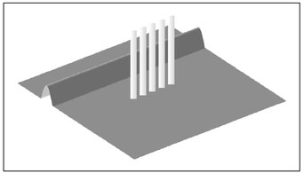
Figure 6.16. Illustration of a configuration of a row of cylinders that could produce a scattered wave that is different from that which is produced by either a single cylinder (Fig. 6.14) or a wall (Fig. 6.15).
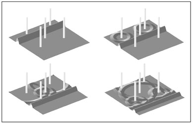
Figure 6.17. Elapsed time sequence of an incident wave crest scattered by five vertical circular cylinders.
The scattering becomes somewhat more complicated when multiple scattering objects exist. Whenever the incident crest encounters a scattering object, a scattered wave will be created and, for multiple scattering objects, there will be multiple scattered waves. Figure 6.17 illustrates an elapsed time sequence of the incident wave scattering from five staggered vertical cylinders. When the incident wave strikes a cylinder, a scattered wave is generated. As the incident wave travels shoreward, the scattered wave propagates radially outward from the cylinder. With each additional cylinder that the incident wave contacts, another circular scattered wave crest is spawned.
For the scattering from a single cylinder (Fig. 6.14), it was assumed that there was a negligible loss of incident wave amplitude (or energy) due to the scattering. With the addition of more scatterers, each drawing a small amount of energy from the incident wave, there can be a noticeable loss of incident wave energy as it propagates past more scattering objects. This loss of incident wave energy is depicted in Fie. 6.17.
After the incident wave has propagated beyond the last scattering objects, there are five scattered circular waves. There are some points where the crests from two scattered waves coincide. At these points there is a local increase in amplitude resulting from the superposition of the two crests. This is called constructive interference. In the preceding examples, only incident and scattered wave crests were considered. If the incident wave was taken to be both a crest and an adjacent trough, then there would be both scattered crests and troughs represented in the illustrations. This admits the possibility that there could be coincident troughs and this again would be constructive interference. There could also be points where the trough from one scattered wave coincides with a crest from another scattered wave. If these have the same amplitude, there would locally be a total cancellation of the two scattered waves. When the amplitudes differ, the superposition of crest and trough will locally diminish the amplitude. The amplitude reduction caused by the superposition of a crest from one wave and trough to another is called destructive interference.
The scattering sequence depicted in Fig. 6.17 considers five scattering objects, but there is only a single scatter from each object. A scattered wave from one object can again be scattered from another object. This is called multiple scattering. Multiple scattering from two vertical cylinders is shown in Fig. 6.18. Here, the incident wave is not shown. The two cylinders are labeled 1 and 2, and it is assumed that the incident wave is propagating in a direction such that it encounters cylinder 1 prior to cylinder 2. The scattering of the incident wave first produces a circular crest radiating outward from cylinder 1 (Fig. 6.18a). At a later time (Fig. 6.18b), there is scattering of the incident wave by cylinder 2 and, as shown, the scattered wave from cylinder 1 has reached cylinder 2. The scattered wave from cylinder 1 is scattered by cylinder 2 producing two outgoing crests from cylinder 2 (Fig. 6.18c), one from the scattering of the incident wave and the second from the scattering of the scattered wave from cylinder 1. Although not shown, there will be an infinite number of multiple scatters. The scattered wave from cylinder 2 will be scattered by cylinder 1, the scattered wave created by cylinder 2 from the scattered wave off of cylinder 1 will again be scattered by cylinder 1, and so on.
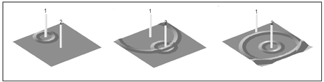
Figure 6.18. Illustration of the first sequence of multiple scattering events from two vertical cylinders. First, (a) the incident wave is scattered by cylinder 1, then (b) the incident wave is scattered by cylinder 2, and finally (c) the scattered wave from cylinder 1 is scattered by cylinder 2.
The scattering from a single object (Fig. 6.14) causes a small redistribution of wave energy. It is also clear that there is some redistribution in the directions of wave propagation. Some of the energy of the incident wave that is propagating in only one direction (here, presumed shoreward) is lost to a scattered wave that propagates in many different directions. When many scattering objects are present (Fig. 6.17) and with multiple scattering (Fig. 6.18), more energy is lost from the primary direction of propagation and is converted to waves propagating in other directions. When a sufficient number of scattering objects is present, there will no longer be a preferred direction of propagation. At this point, the character of the incident wave is lost and there will be waves propagating in all possible directions. This phenomenon is known as Rayleigh scattering and, based on the foregoing discussion, the occurrence of Rayleigh scattering will depend on the number, size, and spacing of scattering objects. There is one additional parameter that is associated with the occurrence of Rayleigh scattering—the wavelength (Sect. 6.1) of the incident wave. The influence of wavelength on Rayleigh scattering can be understood by considering the rolling of a ball through uniformly spaced vertical cylinders of a certain size. If these cylinders are small and far apart, it is likely that this ball will simply pass straight through this obstacle course without encountering any cylinders. This is analogous to no redirection of the incident wave. Conversely, if the cylinders are quite large and/or close together, the ball could be too large to pass through any of the gaps between the cylinders. Here, there is a redirection of the ball but this is not Rayleigh scattering since this special type of scattering is associated with the redirection of an incident wave into scattered waves in all possible directions. The analog to Rayleigh scattering can occur for any cylinder size and spacing (provided that these cylinders do not touch each other) by selecting a ball of appropriate size. In this analogy, the diameter of the ball serves the same function as wavelength in Rayleigh scattering. For scattering objects of any size and spacing, there is some wavelength for which Rayleigh scattering can occur.
With an understanding of Rayleigh scattering, it is possible to answer the question: Why is the sky blue? Standing on Earth and looking away from the sun (the source of light) everything should be black. The reason the Earth's atmosphere is blue is Rayleigh scattering. The light from the sun is scattered in all directions by the gases in the atmosphere. This answer is straightforward. However, the sun is yellow, so why isn't the sky yellow? The color white is the superposition of all colors in the visible spectrum. The sun is predominately composed of white light with a little extra yellow added. This is identical to making yellow paint by adding some yellow tint to a white base. Light is a wave, in fact it is a transverse wave (Sect. 6.2.1), and each color has a unique wavelength. Each color within the spectrum of sunlight is scattered to a greater or lesser extent depending on its wavelength. By far the most abundant gas in the Earth's atmosphere is nitrogen. For the size of nitrogen molecules and their spacing in the atmosphere, the wavelength that will be scattered by nitrogen is that associated with the color blue. If the Earth's atmosphere was composed primarily of some gas other than nitrogen, the sky could be a different color.
In geophysics, in general, waves must be generated by some form of localized disturbance. Artificially, it is impossible to create any waves of global proportions. Thus, waves created in geophysics can be considered as being generated by point sources. Furthermore, there are basically only two forms of energy that can be used to generate waves and the waves generated by these energy forms are known as mechanical and electromagnetic waves.
Mechanical waves are generated by a mechanical movement. Sound waves are mechanical waves and they can be created by striking one object with another or using some force to drive a surface such as in a loud speaker. Sound waves are longitudinal waves, but there also are mechanical waves, which are transverse. Consider a string fixed at one end and being 'shaken' up-and-down at the other end. Obviously, the movement of the string is up and down while the wave propagates along the string. This is a tranverse wave with a vertical polarization. Had the string been shaken back-and-forth, it would also create a transverse wave but with a horizontal polarization.
Electromagnetic waves can be generated in a number of ways. Light is an electromagnetic wave and it can be generated by heat. For instance, a fire generates light from heat. Radio waves are also electromagnetic waves and they are commonly generated by antennas. Electromagnetic waves are transverse waves.
In addition to characterizing waves and exploring some fundamental properties of waves, there are two more basic concepts that are important to the exploitation of waves in geophysics. These are plane waves and pulses.
Comparing Figs. 6.1 and 6.3, there is a noticeable difference between the two wave forms. In Fig. 6.3, the wave crests (and troughs) are parallel, while in Fig. 6.1 the crests (and troughs) appear as concentric circles. Examining a particular wave crest in Fig. 6.3, at any point along a given wave crest, the direction of wave propagation is perpendicular to the line defined by the crest. The direction of propagation can be indicated by an arrow, as shown in Fig. 6.19a, and these arrows are called rays. A ray defines the local direction of wave propagation.
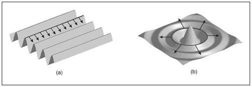
Figure 6.19. Illustration of rays for waves with (a) parallel crests and (b) concentric, circular crests.
Examining Fig. 6.1 in a similar manner, it is evident that rays all radiate outward from the center of a circle (Fig. 6.19b). This pattern of rays is characteristic of a point source. A wave characterized by having all its rays parallel is known as a plane wave. The wave form shown in Fig. 6.3 is a plane wave. Plane waves have some desirable properties in geophysics, A laser is a light source that produces a beam of light that remains at a constant diameter. This is quite different from a more conventional source of light such as a bulb that behaves like a point source and produces rays in all directions. The rays of light produced by a laser are all parallel and, consequently, laser light is a plane wave. It is the special characteristics of plane waves that are responsible for the ability to create holograms using lasers. These special properties are also extremely useful in geophysics.
Unfortunately in geophysics, there is no source analogous to a laser that is capable of directly generating a plane wave. However, plane waves can be synthesized from many point sources. This synthesis is illustrated in Fig. 6.20 where the superposition of waves from many point sources distributed along a line is shown. In terms of the water wave analogy discussed earlier, this synthesis is equivalent to dropping many pebbles into the water such that each strikes the water surface simultaneously and at uniform intervals along a line. This synthesis yields a pattern of crests and troughs that more closely resembles a plane wave (Fig. 6.3) than a wave from any of the individual point sources (Fig. 6.1).
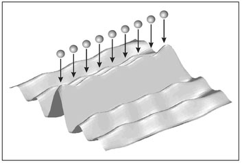
Figure 6.20. Illustration of the approximate synthesis of a plane wave from multiple point sources.
The reason this works is constructive and destructive interference. Figure 6.21 shows a pattern of wave crests and troughs from two point sources. The concentric crests are indicated by the solid lines and between the crests are troughs drawn as dashed lines. Along a line midway between the two sources (the dotted line), there are three points where crests and two points where troughs from both sources coincide. This will produce constructive interference at these points and, for the spacing between point sources shown in this figure, there is no destructive interference.
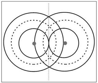
Figure 6.21. Illustration of the superposition crests (solid lines) and troughs (dashed lines) from two point sources.
The actual superposition of the waves from these two point sources is given in Fig. 6.22. Comparing this figure with Fig. 6.1, it is clear that the wave crests have been locally 'flattened' in the area between the two sources.
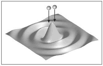
Figure 6.22. Illustration of the locally flattened curvature of circular crests rom the superposition of two point sources.
In Figs. 6.21 and 6.22, there is no destructive interference. This is a result of the close spacing of the point sources. Destructive interference will occur when two point sources have a greater spacing. Figure 6.23 displays the wave form resulting from the superposition of two point sources. This figure is similar to Fig. 6.22 except that, in this case, the point sources are farther apart.
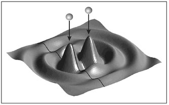
Figure 6.23. The wave form resulting from the superposition of two point sources. The spacing between the point sources is greater here than for the two point sources used in Fig. 6.22.
The wave form shown here differs from that shown in Fig. 6.22 because, with a different point source spacing, there is a change in the pattern of constructive and destructive interference. The contribution of destructive interference is illustrated in Fig. 6.24. These plots show the contribution of the two points sources and their sum along the solid line annotated on Fig. 6.23. This line passes through one of the point sources and the contribution from this source is drawn as a solid line. The individual contribution from the far source is drawn as a dashed line and the sum of these two sources is drawn as a dotted line. Here, there are locations where a crest from one point source coincides with a trough from the other point source. At these locations there is destructive interference. In other locations, there is constructive interference. The net result is a pattern of uniformly spaced crests and troughs that exhibits a much lower loss of amplitude than is typical of geometric spreading from a single point source.
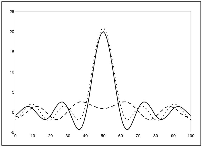
Figure 6.24. Plots of amplitude versus position along the line shown on Fig. 6.23 for the near point source (solid line), the far point source (dashed line), and the superposition of the two point sources (dotted line).
By using many point sources uniformly distributed along a line, an approximate plane wave can be generated. As illustrated in Fig. 6.20, this synthesized wave is characterized by a pattern of near-parallel crests and troughs that propagate without loss of amplitude. This synthesis is made possible by the constructive and destructive interferences among the many point sources. For a plane wave to be synthesized in this manner, the point sources must be distributed along a line and they must be spaced no further than one-half of a wavelength apart.
In introducing Fig. 6.3, it was compared to water waves approaching a beach. It is clear that such water waves appear to be plane waves. Actually water waves of this type are generated by a point source very far away from the beach. The source is, in fact, so far away that the curvature of the circular crests and troughs cannot be noticed. This is analogous to the locally flat Earth assumption used in gravity (Sect. 2.4) and magnetometry.
Pulses are also very important in geophysics. A pulse is a result of energy applied over a very, very short time. In Sect. 6.1, the digital tape measure was introduced (Fig. 6.2) and it was stated that distance can be determined by measuring travel time. Had the energy been released slowly by the digital tape measure and with an amplitude that increased gradually over time, it could be expected that there would be some ambiguity as to the precise time the sound pulse that bounced off the wall was actually detected by the digital tape measure. Any uncertainty in arrival time would result in an uncertainty in computed distance. A similar experiment would be, knowing the speed that electrons travel through a wire, trying to determine the length of wire between a light switch and a light bulb by turning of the switch and then measuring the elapsed time before the light goes out. Electrons travel through wire incredibly fast, however, and even with a very accurate clock and a precise switch, this experiment would fail. The reason for this failure is that a light bulb continues to glow for a short time after the switch has been turned off. Even though this glowing time is brief, it is still much longer than the time required for the signal from the switch to reach the bulb. The problem here is the lack of a sufficiently sharp (short duration) pulse.
Since pulses are used to measure travel time, the problems associated with pulses impact geophysical measurements. A perfect pulse is defined to be an infinite amplitude applied over an infinitesimally short time (Fig. 6.25). Clearly, perfect pulses cannot be created since their creation requires the application of infinite amplitude. Furthermore, is a pulse really a wave since, as shown in Fig. 6.25, it does exhibit the oscillatory behavior that is characteristic of waves (Fig. 6.5)?
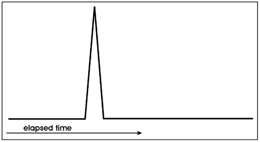
Figure 6.25. Stylized illustration of a pulse.
A pulse is truly a wave and this fact becomes evident when examining the means by which a pulse can be synthesized. A perfect pulse is actually the superposition of an infinite number of waves of different frequencies where all of these waves are in phase (Sect. 6.1) at one point. Now consider the superposition of two frequencies as shown in Fig. 6.26. The waves at the two individual frequencies are drawn as the dashed and dotted lines and their superposition is drawn as a solid line.
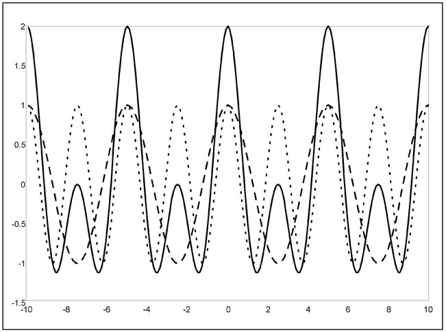
Figure 6.26. Illustration of the superposition of waves having two different frequencies. The higher frequency (dotted line) is twice that of the lower frequency (dashed line), and their superposition is drawn as the solid line.
Note that there is both constructive and destructive interference that reinforce certain crests and troughs while eliminating others. By adding progressively more frequencies, there will always be constructive interference at the time when all waves are in phase (here taken to be time equal to zero) but there will also be less constructive and more destructive interference elsewhere. This fact is demonstrated in Fig. 6.27 where the superposition of 3, 9, and 65 frequencies are shown. With the addition of more frequencies, the superposition becomes more pulse-like and less wave-like until this superposition yields a near-perfect pulse.

Figure 6.27 The superposition of waves with (a) three, (b) nine, and (c) sixty-five frequencies.
The problem of computing distance from measured travel with an imperfect pulse becomes more apparent within the context of Fig. 6.27. For a small number of frequencies (Fig. 6.27a), the pulse is poorly approximated and there are many crests. The largest of these is referred to as the main lobe and all others are side lobes. If there are many lobes, the amplitude of the main lobe is not significantly larger than some side lobes. This introduces an ambiguity in discriminating the arrival time of the main lobe from those of the side lobes. There is a different travel time associated with each lobe so that the computed distance will be different depending on the lobe selected for travel time. Travel time ambiguity diminishes for approximate pulses composed of more frequencies (Figs. 6.27b and 6.27c). Here, the amplitude of the main lobe becomes much larger than any side lobes and is more easily discriminated.
Having 'assembled' a pulse, the problem of decomposing a pulse can be addressed. This is done with the knowledge that it is impossible to generate a perfect pulse. Think of striking one object against another. Depending upon the nature of the materials of the two objects and their size, the sound heard may be high, low, or mid-range. If a perfect pulse is generated, all tones would be heard equally. Thus, there are frequencies missing and the wave form might look like those shown in Figs. 6.27a or 6.27b. In geophysics, it is therefore necessary to function with imperfect pulses and recognize the consequences and limitations of such.
There is a relationship between pulses and point sources. A pulse is a wave where all the energy is applied over a very short time. Similarly, a point source is a source where all the energy is applied over a very limited area in space. In one dimension, a point source could be described by Fig. 6.25 with distance replacing time on the horizontal axis. The same method of analysis used to demonstrate that a pulse is a superposition of waves of many frequencies (Fig. 6.27) could be used to show that a point source is the superposition of waves having many distinct wavelengths.
1. This type of wave is commonly referred to as tidally driven. This is a misnomer. Tidal forcing actual produces a sloshing motion and is properly called a standing wave.