Materials
The BRDFs and BTDFs introduced in the previous chapter address only part of the problem of describing how a surface scatters light. Although they describe how light is scattered at a particular point on a surface, the renderer needs to determine which BRDFs and BTDFs are present at a point on a surface and what their parameters are. In this chapter, we describe a procedural shading mechanism that addresses this issue.
The basic idea behind pbrt’s approach is that a surface shader is bound to each primitive in the scene. The surface shader is represented by an instance of the Material interface class, which has a method that takes a point on a surface and creates a BSDF object (and possibly a BSSRDF) that represents scattering at the point. The BSDF class holds a set of BxDFs whose contributions are summed to give the full scattering function. Materials, in turn, use instances of the Texture class (to be defined in the next chapter) to determine the material properties at particular points on surfaces. For example, an ImageTexture might be used to modulate the color of diffuse reflection across a surface. This is a somewhat different shading paradigm from the one that many rendering systems use; it is common practice to combine the function of the surface shader and the lighting integrator (see Chapter 14) into a single module and have the shader return the color of reflected light at the point. However, by separating these two components and having the Material return a BSDF, pbrt is better able to handle a variety of light transport algorithms.
9.1 BSDFs
The BSDF class represents a collection of BRDFs and BTDFs. Grouping them in this manner allows the rest of the system to work with composite BSDFs directly, rather than having to consider all of the components they may have been built from. Equally important, the BSDF class hides some of the details of shading normals from the rest of the system. Shading normals, either from per-vertex normals in triangle meshes or from bump mapping, can substantially improve the visual richness of rendered scenes, but because they are an ad hoc construct, they are tricky to incorporate into a physically based renderer. The issues that they introduce are handled in the BSDF implementation.
〈BSDF Declarations〉 + ≡
class BSDF {
public:
〈BSDF Public Methods 573〉
〈BSDF Public Data 573〉
private:
〈BSDF Private Methods 576〉
〈BSDF Private Data 573〉
};
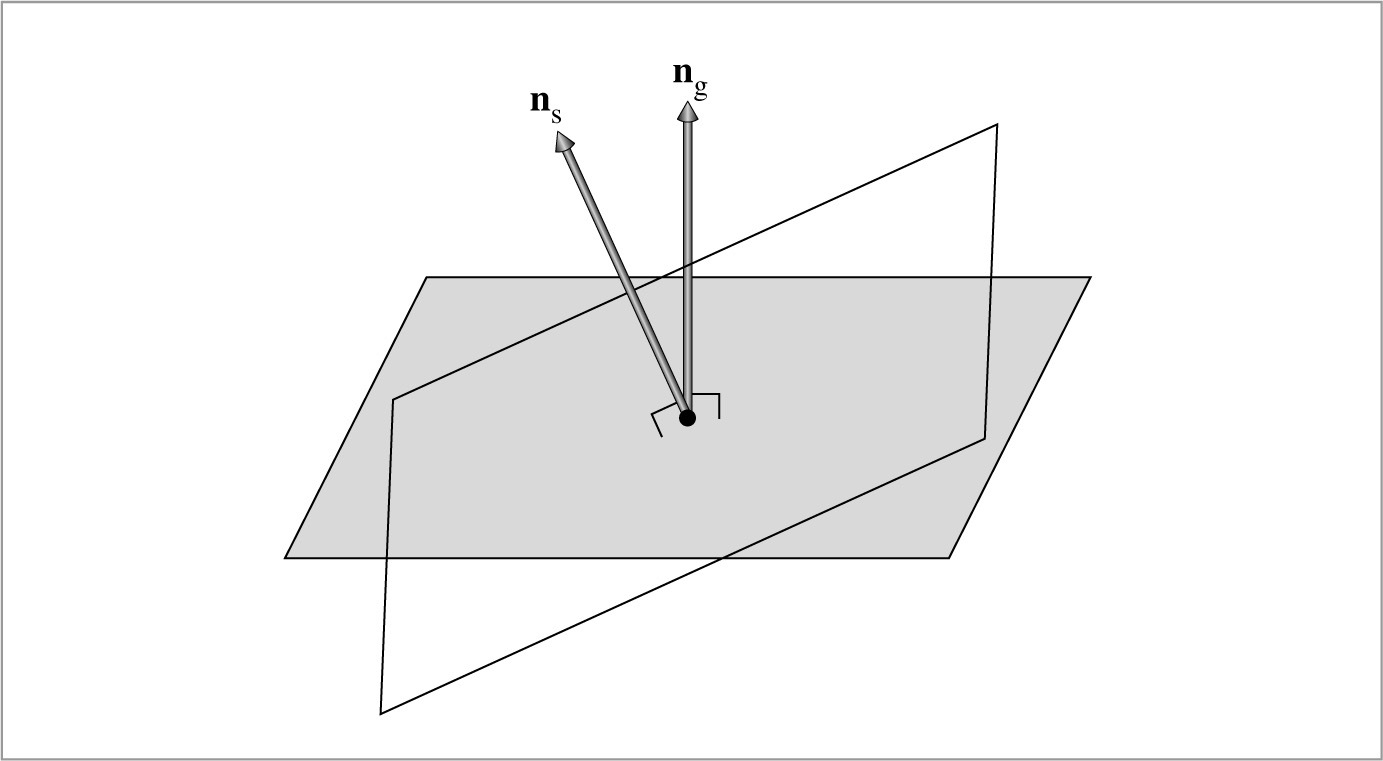
The BSDF constructor takes a SurfaceInteraction object that contains information about the differential geometry at the point on a surface as well as a parameter eta that gives the relative index of refraction over the boundary. For opaque surfaces, eta isn’t used, and a value of one should be provided by the caller. (The default value of one for eta is for just this case.) The constructor computes an orthonormal coordinate system with the shading normal as one of the axes; this coordinate system will be useful for transforming directions to and from the BxDF coordinate system that is described in Figure 8.2. Throughout this section, we will use the convention that ns denotes the shading normal and ng the geometric normal (Figure 9.1).
〈BSDF Public Methods〉 ≡ 572
BSDF(const SurfaceInteraction &si, Float eta = 1)
: eta(eta), ns(si.shading.n), ng(si.n),
ss(Normalize(si.shading.dpdu)), ts(Cross(ns, ss)) { }
〈BSDF Public Data〉 ≡ 572
const Float eta;
〈BSDF Private Data〉 ≡ 572
const Normal3f ns, ng;
const Vector3f ss, ts;
The BSDF implementation stores only a limited number of individual BxDF components. It could easily be extended to allocate more space if more components were given to it, although this isn’t necessary for any of the Material implementations in pbrt thus far, and the current limit of eight is plenty for almost all practical applications.
〈BSDF Public Methods〉 + ≡ 572
void Add(BxDF *b) {
Assert(nBxDFs < MaxBxDFs);
bxdfs[nBxDFs++] = b;
}
〈BSDF Private Data〉 + ≡ 572
int nBxDFs = 0;
static constexpr int MaxBxDFs = 8;
BxDF *bxdfs[MaxBxDFs];
For other parts of the system that need additional information about the particular BRDFs and BTDFs that are present, a method returns the number of BxDFs stored by the BSDF that match a particular set of BxDFType flags.
〈BSDF Public Methods〉 + ≡ 572
int NumComponents(BxDFType flags = BSDF_ALL) const;
The BSDF also has methods that perform transformations to and from the local coordinate system used by BxDFs. Recall that, in this coordinate system, the surface normal is along the z axis (0, 0, 1), the primary tangent is (1, 0, 0), and the secondary tangent is (0, 1, 0). The transformation of directions into “shading space” simplifies many of the BxDF implementations in Chapter 8. Given three orthonormal vectors s, t, and n in world space, the matrix M that transforms vectors in world space to the local reflection space is
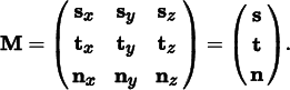
To confirm this yourself, consider, for example, the value of M times the surface normal n, Mn = (s • n, t • n, n • n). Since s, t, and n are all orthonormal, the x and y components of Mn are zero. Since n is normalized, n • n = 1. Thus, Mn = (0, 0, 1), as expected.
In this case, we don’t need to compute the inverse transpose of M to transform normals (recall the discussion of transforming normals in Section 2.8.3). Because M is an orthogonal matrix (its rows and columns are mutually orthogonal), its inverse is equal to its transpose, so it is its own inverse transpose already.
〈BSDF Public Methods〉 + ≡ 572
Vector3f WorldToLocal(const Vector3f &v) const {
return Vector3f(Dot(v, ss), Dot(v, ts), Dot(v, ns));
}
The method that takes vectors back from local space to world space transposes M to find its inverse before doing the appropriate dot products.
〈BSDF Public Methods〉 + ≡ 572
Vector3f LocalToWorld(const Vector3f &v) const {
return Vector3f(ss.x * v.x + ts.x * v.y + ns.x * v.z,
ss.y * v.x + ts.y * v.y + ns.y * v.z,
ss.z * v.x + ts.z * v.y + ns.z * v.z);
}
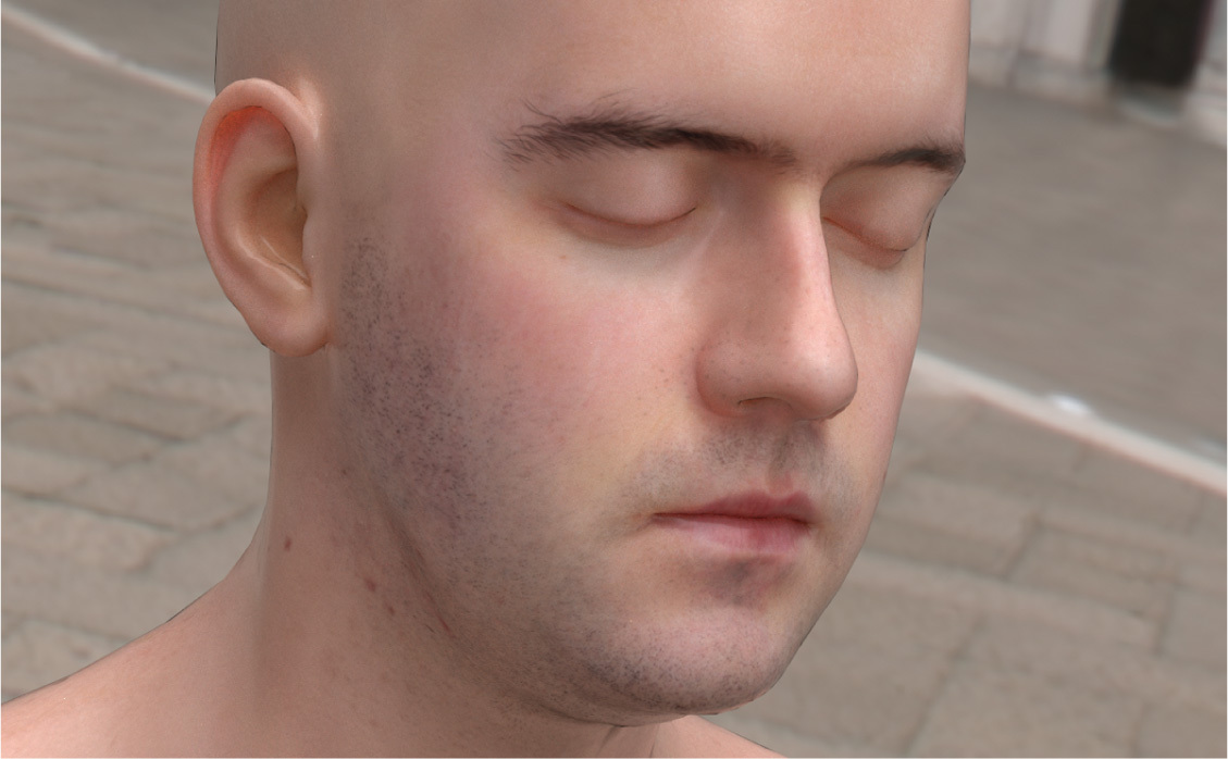
Shading normals can cause a variety of undesirable artifacts in practice (Figure 9.2). Figure 9.2(a) shows a light leak: the geometric normal indicates that ωi and ωo lie on opposite sides of the surface, so if the surface is not transmissive, the light should have no contribution. However, if we directly evaluate the scattering equation, Equation (5.9), about the hemisphere centered around the shading normal, we will incorrectly incorporate the light from ωi. This case demonstrates that ns can’t just be used as a direct replacement for ng in rendering computations.
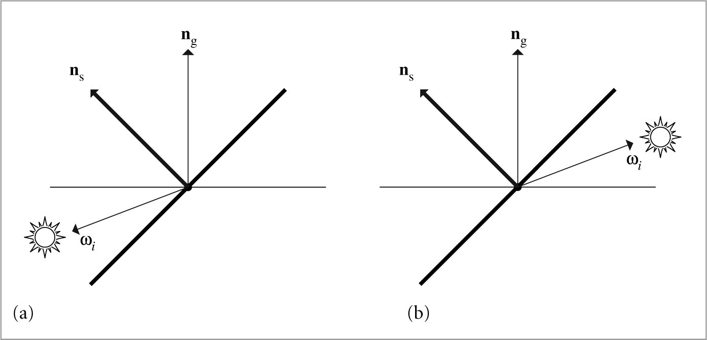
Figure 9.2(b) shows a similar tricky situation: the shading normal indicates that no light should be reflected to the viewer, since it is not in the same hemisphere as the illumination, while the geometric normal indicates that they are in the same hemisphere. Direct use of ns would cause ugly black spots on the surface where this situation happens.
Fortunately, there is an elegant solution to these problems. When evaluating the BSDF, we can use the geometric normal to decide if we should be evaluating reflection or transmission: if ωi and ωo lie in the same hemisphere with respect to ng, we evaluate the BRDFs, and otherwise we evaluate the BTDFs. In evaluating the scattering equation, however, the dot product of the normal and the incident direction is still taken with the shading normal rather than the geometric normal.
Now it should be clear why pbrt requires BxDFs to evaluate their values without regard to whether ωi and ωo are in the same or different hemispheres. This convention means that light leaks are avoided, since we will only evaluate the BTDFs for the situation in Figure 9.2(a), giving no reflection for a purely reflective surface. Similarly, black spots are avoided since we will evaluate the BRDFs for the situation in Figure 9.2(b), even though the shading normal would suggest that the directions are in different hemispheres.
Given these conventions, the method that evaluates the BSDF for a given pair of directions follows directly. It starts by transforming the world space direction vectors to local BSDF space and then determines whether it should use the BRDFs or the BTDFs. It then loops over the appropriate set and evaluates the sum of their contributions.
〈BSDF Method Definitions〉 ≡
Spectrum BSDF::f(const Vector3f &woW, const Vector3f &wiW,
BxDFType flags) const {
Vector3f wi = WorldToLocal(wiW), wo = WorldToLocal(woW);
bool reflect = Dot(wiW, ng) * Dot(woW, ng) > 0;
Spectrum f(0.f);
for (int i = 0; i < nBxDFs; ++i)
if (bxdfs[i]- > MatchesFlags(flags) &&
((reflect && (bxdfs[i]- > type & BSDF_REFLECTION)) 
(!reflect && (bxdfs[i]- > type & BSDF_TRANSMISSION))))
f + = bxdfs[i]- > f(wo, wi);
return f;
}
pbrt also provides BSDF methods that return the BSDF’s reflectances. (Recall the definition of reflectance in Section 8.1.1.) The two corresponding methods just loop over the BxDFs and sum the values returned by their BxDF::rho() methods; their straightforward implementations aren’t included here. These methods take arrays of samples for BxDFs for use in Monte Carlo sampling algorithms if needed (recall the BxDF::rho() interface defined in Section 8.1.1, which takes such samples as well.)
〈BSDF Public Methods〉 + ≡ 572
Spectrum rho(int nSamples, const Point2f *samples1,
const Point2f *samples2, BxDFType flags = BSDF_ALL) const;
Spectrum rho(const Vector3f &wo, int nSamples, const Point2f *samples,
BxDFType flags = BSDF_ALL) const;
9.1.1 BSDF Memory management
For each ray that intersects geometry in the scene, one or more BSDF objects will be created by the Integrator in the process of computing the radiance carried along the ray. (Integrators that account for multiple interreflections of light will generally create a number of BSDFs along the way.) Each of these BSDFs in turn has a number of BxDFs stored inside it, as created by the Materials at the intersection points.
A naïve implementation would use new and delete to dynamically allocate storage for both the BSDF as well as each of the BxDFs that it holds. Unfortunately, such an approach would be unacceptably inefficient—too much time would be spent in the dynamic memory management routines for a series of small memory allocations. Instead, the implementation here uses a specialized allocation scheme based on the MemoryArena class described in Section A.4.3.1 A MemoryArena is passed into methods that allocate memory for BSDFs. For example, the SamplerIntegrator::Render() method creates a MemoryArena for each image tile and passes it to the integrators, which in turn pass it to the Material.
For the convenience of code that allocates BSDFs and BxDFs (e.g., the Materials in this chapter), there is a macro that hides some of the messiness of using the memory arena. Instead of using the new operator to allocate those objects like this:
BSDF *b = new BSDF;
BxDF *lam = new LambertianReflection(Spectrum(0.5f));
code should instead be written with the ARENA_ALLOC() macro, like this:
BSDF *b = ARENA_ALLOC(arena, BSDF);
BxDF *lam = ARENA_ALLOC(arena, LambertianReflection)(Spectrum(0.5f));
where arena is a MemoryArena.
The ARENA_ALLOC() macro uses the placement operator new to run the constructor for the object at the returned memory location.
〈Memory Declarations〉 ≡
#define ARENA_ALLOC(arena, Type) new (arena.Alloc(sizeof(Type))) Type
The BSDF destructor is a private method in order to ensure that it isn’t inadvertently called (e.g., due to an attempt to delete a BSDF). Making the destructor private ensures a compile time error if it is called. Trying to delete memory allocated by the MemoryArena could lead to errors or crashes, since a pointer to the middle of memory managed by the MemoryArena would be passed to the system’s dynamic memory freeing routine.
In turn, an implication of the allocation scheme here is that BSDF and BxDF destructors are never executed. This isn’t a problem for the ones currently implemented in the system.
〈BSDF Private Methods〉 ≡ 572
~ BSDF() { }
9.2 Material interface and implementations
The abstract Material class defines the interface that material implementations must provide. The Material class is defined in the files core/material.h and core/material.cpp.
〈Material Declarations〉 ≡
class Material {
public:
〈Material Interface 577〉
};
A single method must be implemented by Material s: ComputeScatteringFunctions(). This method is given a SurfaceInteraction object that contains geometric properties at an intersection point on the surface of a shape. The method’s implementation is responsible for determining the reflective properties at the point and initializing the SurfaceInteraction::bsdf member variable with a corresponding BSDF class instance. If the material includes subsurface scattering, then the SurfaceInteraction::bssrdf member should be initialized as well. (It should otherwise be left unchanged from its default nullptr value.) The BSSRDF class that represents subsurface scattering functions is defined later, in Section 11.4, after the foundations of volumetric scattering have been introduced.
Three additional parameters are passed to this method:
• A MemoryArena, which should be used to allocate memory for BSDFs and BSSRDFs.
• The TransportMode parameter, which indicates whether the surface intersection was found along a path starting from the camera or one starting from a light source; this detail has implications for how BSDFs and BSSRDFs are evaluated—see Section 16.1.
• Finally, the allowMultipleLobes parameter indicates whether the material should use BxDFs that aggregate multiple types of scattering into a single BxDF when such BxDFs are available. (An example of such a BxDF is FresnelSpecular, which includes both specular reflection and transmission.) These BxDFs can improve the quality of final results when used with Monte Carlo light transport algorithms but can introduce noise in images when used with the DirectLightingIntegrator and WhittedIntegrator. Therefore, the Integrator is allowed to control whether such BxDFs are used via this parameter.
〈Material Interface〉 ≡ 577
virtual void ComputeScatteringFunctions(SurfaceInteraction *si,
MemoryArena &arena, TransportMode mode,
bool allowMultipleLobes) const = 0;
Since the usual interface to the intersection point used by Integrators is through an instance of the SurfaceInteraction class, we will add a convenience method ComputeScatteringFunctions() to that class. Its implementation first calls the Surface Interaction’s ComputeDifferentials() method to compute information about the projected size of the surface area around the intersection on the image plane for use in texture antialiasing. Next, it forwards the request to the Primitive, which in turn will call the corresponding ComputeScatteringFunctions() method of its Material. (See, for example, the GeometricPrimitive::ComputeScatteringFunctions() implementation.)
〈SurfaceInteraction Method Definitions〉 + ≡
void SurfaceInteraction::ComputeScatteringFunctions(
const RayDifferential &ray, MemoryArena &arena,
bool allowMultipleLobes, TransportMode mode) {
ComputeDifferentials(ray);
primitive- > ComputeScatteringFunctions(this, arena, mode,
allowMultipleLobes);
}
9.2.1 Matte material
The MatteMaterial material is defined in materials/matte.h and materials/matte.cpp. It is the simplest material in pbrt and describes a purely diffuse surface.
〈MatteMaterial Declarations〉 ≡
class MatteMaterial : public Material {
public:
〈MatteMaterial Public Methods 578〉
private:
〈MatteMaterial Private Data 578〉
};
This material is parameterized by a spectral diffuse reflection value, Kd, and a scalar roughness value, sigma. If sigma has the value zero at the point on a surface, Matte Material creates a LambertianReflection BRDF; otherwise, the OrenNayar model is used. Like all of the other Material implementations in this chapter, it also takes an optional scalar texture that defines an offset function over the surface. If its value is not nullptr, this texture is used to compute a shading normal at each point based on the function it defines. (Section 9.3 discusses the implementation of this computation.) Figure 8.14 in the previous chapter shows the MatteMaterial material with the dragon model.
〈MatteMaterial Public Methods〉 ≡ 578
MatteMaterial(const std::shared_ptr < Texture < Spectrum > > &Kd,
const std::shared_ptr < Texture < Float > > &sigma,
const std::shared_ptr < Texture < Float > > &bumpMap)
: Kd(Kd), sigma(sigma), bumpMap(bumpMap) { }
〈MatteMaterial Private Data〉 ≡ 578
std::shared_ptr < Texture < Spectrum > > Kd;
std::shared_ptr < Texture < Float > > sigma, bumpMap;
The ComputeScatteringFunctions() method puts the pieces together, determining the bump map’s effect on the shading geometry, evaluating the textures, and allocating and returning the appropriate BSDF.
〈MatteMaterial Method Definitions〉 ≡
void MatteMaterial::ComputeScatteringFunctions(SurfaceInteraction *si,
MemoryArena &arena, TransportMode mode,
bool allowMultipleLobes) const {
〈Perform bump mapping with bumpMap, if present 579〉
〈Evaluate textures for MatteMaterial material and allocate BRDF 579〉
}
If a bump map was provided to the MatteMaterial constructor, the Material::Bump() method is called to calculate the shading normal at the point. This method will be defined in the next section.
〈Perform bump mapping with bumpMap, if present〉 ≡ 579, 581, 584, 701
if (bumpMap)
Bump(bumpMap, si);
Next, the Textures that give the values of the diffuse reflection spectrum and the roughness are evaluated; texture implementations may return constant values, look up values from image maps, or do complex procedural shading calculations to compute these values (the texture evaluation process is the subject of Chapter 10). Given these values, all that needs to be done is to allocate a BSDF and then allocate the appropriate type of Lambertian BRDF and provide it to the BSDF. Because Textures may return negative values or values otherwise outside of the expected range, these values are clamped to valid ranges before they are passed to the BRDF constructor.
〈Evaluate textures for MatteMaterial material and allocate BRDF〉 ≡ 579
si- > bsdf = ARENA_ALLOC(arena, BSDF)(*si);
Spectrum r = Kd- > Evaluate(*si).Clamp();
Float sig = Clamp(sigma- > Evaluate(*si), 0, 90);
if (!r.IsBlack()) {
if (sig == 0)
si- > bsdf- > Add(ARENA_ALLOC(arena, LambertianReflection)(r));
else
si- > bsdf- > Add(ARENA_ALLOC(arena, OrenNayar)(r, sig));
}
9.2.2 Plastic material
Plastic can be modeled as a mixture of a diffuse and glossy scattering function with parameters controlling the particular colors and specular highlight size. The parameters to PlasticMaterial are two reflectivities, Kd and Ks, which respectively control the amounts of diffuse reflection and glossy specular reflection.
Next is a roughness parameter that determines the size of the specular highlight. It can be specified in two ways. First, if the remapRoughness parameter is true, then the given roughness should vary from zero to one, where the higher the roughness value, the larger the highlight. (This variant is intended to be fairly user-friendly.) Alternatively, if the parameter is false, then the roughness is used to directly initialize the microfacet distribution’s α parameter (recall Section 8.4.2).
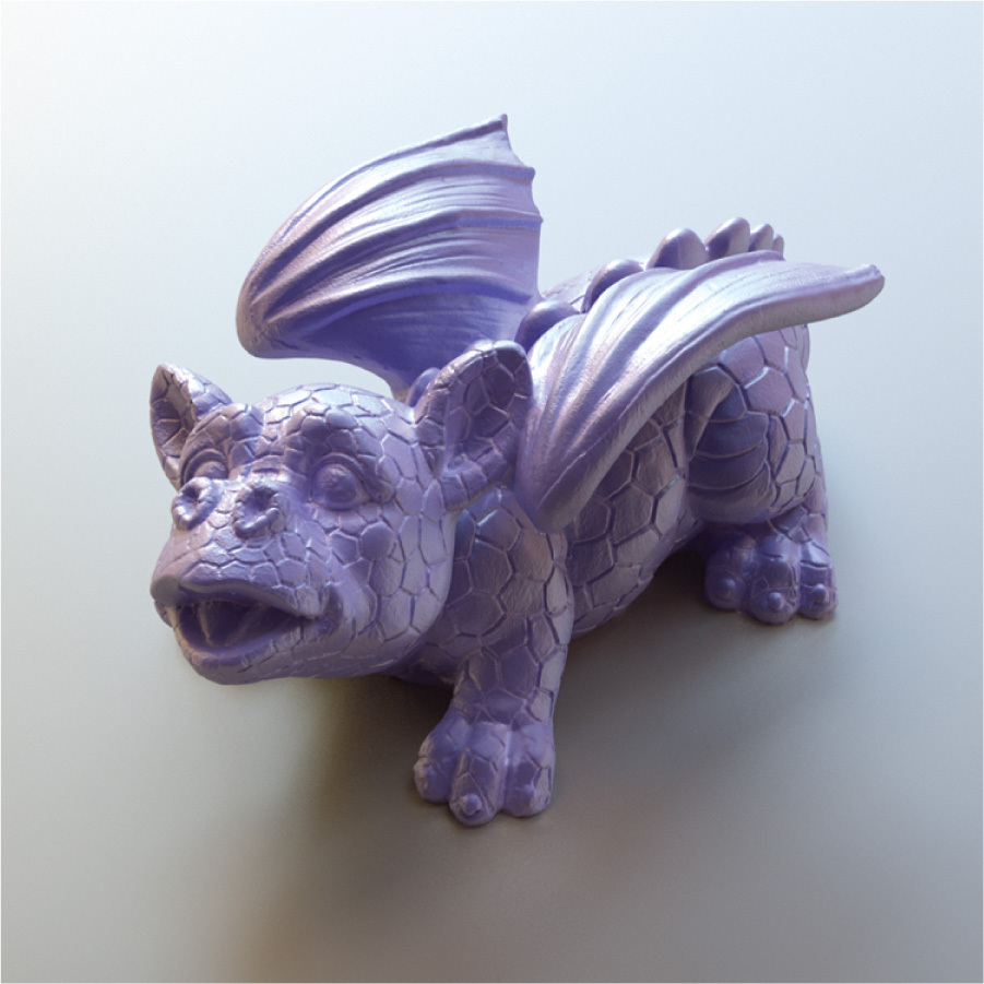
Figure 9.3 shows a plastic dragon. PlasticMaterial is defined in materials/plastic.h and materials/plastic.cpp.
〈PlasticMaterial Declarations〉 ≡
class PlasticMaterial : public Material {
public:
〈PlasticMaterial Public Methods 580〉
private:
〈PlasticMaterial Private Data 580〉
};
〈PlasticMaterial Public Methods〉 ≡ 580
PlasticMaterial(const std::shared_ptr < Texture < Spectrum > > &Kd,
const std::shared_ptr < Texture < Spectrum > > &Ks,
const std::shared_ptr < Texture < Float > > &roughness,
const std::shared_ptr < Texture < Float > > &bumpMap,
bool remapRoughness)
: Kd(Kd), Ks(Ks), roughness(roughness), bumpMap(bumpMap),
remapRoughness(remapRoughness) { }
〈PlasticMaterial Private Data〉 ≡ 580
std::shared_ptr < Texture < Spectrum > > Kd, Ks;
std::shared_ptr < Texture < Float > > roughness, bumpMap;
const bool remapRoughness;
The PlasticMaterial::ComputeScatteringFunctions() method follows the same basic structure as MatteMaterial::ComputeScatteringFunctions(): it calls the bump-mapping function, evaluates textures, and then allocates BxDFs to use to initialize the BSDF.
〈PlasticMaterial Method Definitions〉 ≡
void PlasticMaterial::ComputeScatteringFunctions(
SurfaceInteraction *si, MemoryArena &arena, TransportMode mode,
bool allowMultipleLobes) const {
〈Perform bump mapping with bumpMap, if present 579〉
si- > bsdf = ARENA_ALLOC(arena, BSDF)(*si);
〈Initialize diffuse component of plastic material 581〉
〈Initialize specular component of plastic material 581〉
}
In Material implementations, it’s worthwhile to skip creation of BxDF components that do not contribute to the scattering at a point. Doing so saves the renderer unnecessary work later when it’s computing reflected radiance at the point. Therefore, the Lambertian component is only created if kd is non-zero.
〈Initialize diffuse component of plastic material〉 ≡ 581
Spectrum kd = Kd- > Evaluate(*si).Clamp();
if (!kd.IsBlack())
si- > bsdf- > Add(ARENA_ALLOC(arena, LambertianReflection)(kd));
As with the diffuse component, the glossy specular component is skipped if it’s not going to make a contribution to the overall BSDF.
〈Initialize specular component of plastic material〉 ≡ 581
Spectrum ks = Ks- > Evaluate(*si).Clamp();
if (!ks.IsBlack()) {
Fresnel *fresnel = ARENA_ALLOC(arena, FresnelDielectric)(1.f, 1.5f);
〈Create microfacet distribution distrib for plastic material 581〉
BxDF *spec =
ARENA_ALLOC(arena, MicrofacetReflection)(ks, distrib, fresnel);
si- > bsdf- > Add(spec);
}
〈Create microfacet distribution distrib for plastic material〉 ≡ 581
Float rough = roughness- > Evaluate(*si);
if (remapRoughness)
rough = TrowbridgeReitzDistribution::RoughnessToAlpha(rough);
MicrofacetDistribution *distrib =
ARENA_ALLOC(arena, TrowbridgeReitzDistribution)(rough, rough);
9.2.3 Mix material
It’s useful to be able to combine two Materials with varying weights. The MixMaterial takes two other Materials and a Spectrum-valued texture and uses the Spectrum returned by the texture to blend between the two materials at the point being shaded. It is defined in the files materials/mixmat.h and materials/mixmat.cpp.
〈MixMaterial Declarations〉 ≡
class MixMaterial : public Material {
public:
〈MixMaterial Public Methods 582〉
private:
〈MixMaterial Private Data 582〉
};
〈MixMaterial Public Methods〉 ≡ 582
MixMaterial(const std::shared_ptr < Material > &m1,
const std::shared_ptr < Material > &m2,
const std::shared_ptr < Texture < Spectrum > > &scale)
: m1(m1), m2(m2), scale(scale) { }
〈MixMaterial Private Data〉 ≡ 582
std::shared_ptr < Material > m1, m2;
std::shared_ptr < Texture < Spectrum > > scale;
〈MixMaterial Method Definitions〉 ≡
void MixMaterial::ComputeScatteringFunctions(SurfaceInteraction *si,
MemoryArena &arena, TransportMode mode,
bool allowMultipleLobes) const {
〈Compute weights and original BxDF s for mix material 582〉
〈Initialize si- > bsdf with weighted mixture of BxDFs 583〉
}
MixMaterial::ComputeScatteringFunctions() starts with its two constituent Materials initializing their respective BSDFs.
〈Compute weights and original BxDFs for mix material〉 ≡ 582
Spectrum s1 = scale- > Evaluate(*si).Clamp();
Spectrum s2 = (Spectrum(1.f) - s1).Clamp();
SurfaceInteraction si2 = *si;
m1- > ComputeScatteringFunctions(si, arena, mode, allowMultipleLobes);
m2- > ComputeScatteringFunctions(&si2, arena, mode, allowMultipleLobes);
It then scales BxDFs in the BSDF from the first material, b1, using the ScaledBxDF adapter class, and then scales the BxDFs from the second BSDF, adding all of these BxDF components to si- > bsdf.
It may appear that there’s a lurking memory leak in this code, in that the BxDF *s in si- > bxdfs are clobbered by newly allocated ScaledBxDFs. However, recall that those BxDFs, like the new ones here, were allocated through a MemoryArena and thus their memory will be freed when the MemoryArena frees its entire block of memory.
〈Initialize si- > bsdf with weighted mixture of BxDFs〉 ≡ 582
int n1 = si- > bsdf- > NumComponents(), n2 = si2.bsdf- > NumComponents();
for (int i = 0; i < n1; ++i)
si- > bsdf- > bxdfs[i] =
ARENA_ALLOC(arena, ScaledBxDF)(si- > bsdf- > bxdfs[i], s1);
for (int i = 0; i < n2; ++i)
si- > bsdf- > Add(ARENA_ALLOC(arena, ScaledBxDF)(si2.bsdf- > bxdfs[i], s2));
The implementation of MixMaterial::ComputeScatteringFunctions() needs direct access to the bxdfs member variables of the BSDF class. Because this is the only class that needs this access, we’ve just made MixMaterial a friend of BSDF rather than adding a number of accessor and setting methods.
〈BSDF Private Data〉 + ≡ 572
friend class MixMaterial;
9.2.4 Fourier material
The FourierMaterial class supports measured or synthetic BSDF data that has been tabulated into the directional basis that was introduced in Section 8.6. It is defined in the files materials/fourier.h and materials/fourier.cpp.
〈FourierMaterial Declarations〉 ≡
class FourierMaterial : public Material {
public:
〈FourierMaterial Public Methods〉
private:
〈FourierMaterial Private Data 583〉
};
The constructor is responsible for reading the BSDF from a file and initializing the FourierBSDFTable.
〈FourierMaterial Method Definitions〉 ≡
FourierMaterial::FourierMaterial(const std::string &filename,
const std::shared_ptr < Texture < Float > > &bumpMap)
: bumpMap(bumpMap) {
FourierBSDFTable::Read(filename, &bsdfTable);
}
〈FourierMaterial Private Data〉 ≡ 583
FourierBSDFTable bsdfTable;
std::shared_ptr < Texture < Float > > bumpMap;
Once the data is in memory, the ComputeScatteringFunctions() method’s task is straightforward. After the usual bump-mapping computation, it just has to allocate a FourierBSDF and provide it access to the data in the table.
〈FourierMaterial Method Definitions〉 + ≡
void FourierMaterial::ComputeScatteringFunctions(SurfaceInteraction *si,
MemoryArena &arena, TransportMode mode,
bool allowMultipleLobes) const {
〈Perform bump mapping with bumpMap, if present 579〉
si- > bsdf = ARENA_ALLOC(arena, BSDF)(*si);
si- > bsdf- > Add(ARENA_ALLOC(arena, FourierBSDF)(bsdfTable, mode));
}
9.2.5 Additional materials
Beyond these materials, there are eight more Material implementations available in pbrt, all in the materials/ directory. We will not show all of their implementations here, since they are all just variations on the basic themes introduced in the material implementations above. All take Textures that define scattering parameters, these textures are evaluated in the materials’ respective ComputeScatteringFunctions() methods, and appropriate BxDFs are created and returned in a BSDF. See the documentation on pbrt’s file format for a summary of the parameters that these materials take.
These materials include:
• GlassMaterial: Perfect or glossy specular reflection and transmission, weighted by Fresnel terms for accurate angular-dependent variation.
• MetalMaterial: Metal, based on the Fresnel equations for conductors and the Torrance–Sparrow model. Unlike plastic, metal includes no diffuse component. See the files in the directory scenes/spds/metals/ for measured spectral data for the indices of refraction η and absorption coefficients k for a variety of metals.
• MirrorMaterial: A simple mirror, modeled with perfect specular reflection.
• SubstrateMaterial: A layered model that varies between glossy specular and diffuse reflection depending on the viewing angle (based on the FresnelBlend BRDF).
• SubsurfaceMaterial and KdSubsurfaceMaterial: Materials that return BSSRDFs that describe materials that exhibit subsurface scattering.
• TranslucentMaterial: A material that describes diffuse and glossy specular reflection and transmission through the surface.
• UberMaterial: A “kitchen sink” material representing the union of many of the preceding materials. This is a highly parameterized material that is particularly useful when converting scenes from other file formats into pbrt’s.
Figure 8.10 in the previous chapter shows the dragon model rendered with Glass Material, and Figure 9.4 shows it with the MetalMaterial. Figure 9.5 demonstrates the KdSubsurfaceMaterial.

9.3 Bump mapping
All of the Materials defined in the previous section take an optional floating-point texture that defines a displacement at each point on the surface: each point p has a displaced point p′ associated with it, defined by p′ = p + d(p)n(p), where d(p) is the offset returned by the displacement texture at p and n(p) is the surface normal at p (Figure 9.6). We would like to use this texture to compute shading normals so that the surface appears as if it actually had been offset by the displacement function, without modifying its geometry. This process is called bump mapping. For relatively small displacement functions, the visual effect of bump mapping can be quite convincing. This idea and the specific technique to compute these shading normals in a way that gives a plausible appearance of the actual displaced surface were developed by Blinn (1978).
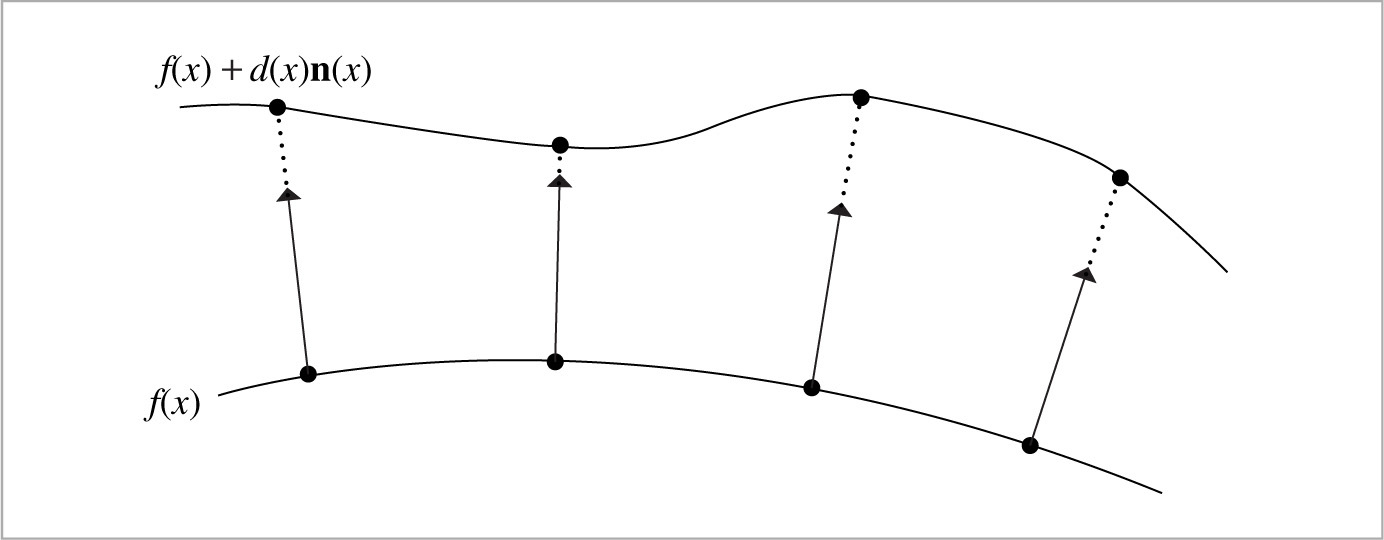
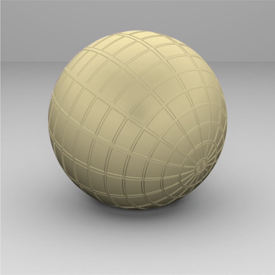
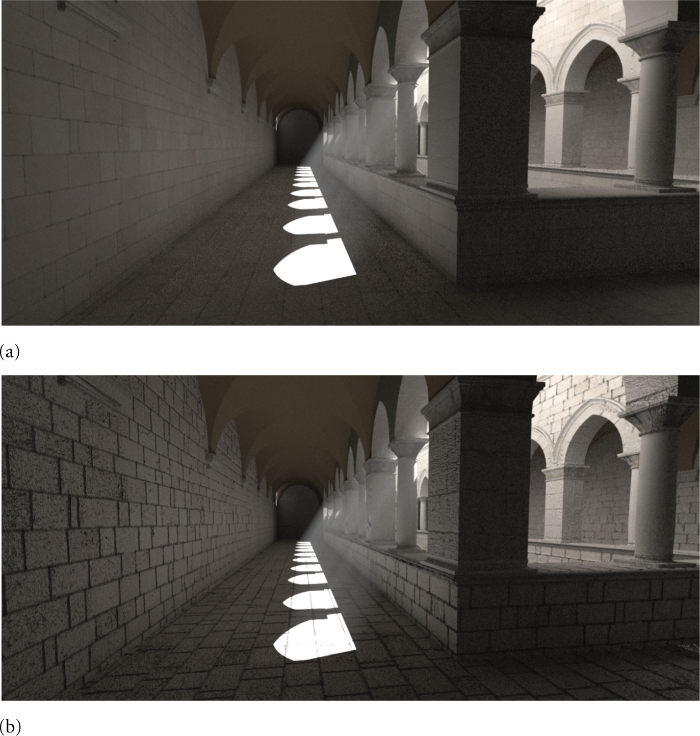
Figure 9.7 shows the effect of applying bump mapping defined by an image map of a grid of lines to a sphere. A more complex example is shown in Figure 9.8, which shows a scene rendered with and without bump mapping. There, the bump map gives the appearance of a substantial amount of detail in the walls and floors that isn’t actually present in the geometric model. Figure 9.9 shows one of the image maps used to define the bump function in Figure 9.8.

The Material::Bump() method is a utility routine for use by Material implementations. It is responsible for computing the effect of bump mapping at the point being shaded given a particular displacement Texture. So that future Material implementations aren’t required to support bump mapping with this particular mechanism (or at all), we’ve placed this method outside of the hard-coded material evaluation pipeline and left it as a function that particular material implementations can call on their own.
The implementation of Material::Bump() is based on finding an approximation to the partial derivatives ∂p/∂u and ∂p/∂v of the displaced surface and using them in place of the surface’s actual partial derivatives to compute the shading normal. (Recall that the surface normal is given by the cross product of these vectors, n = ∂p/∂u × ∂p/∂v.) Assume that the original surface is defined by a parametric function p(u, v), and the bump offset function is a scalar function d(u, v). Then the displaced surface is given by

where n(u, v) is the surface normal at (u, v).
The partial derivatives of this function can be found using the chain rule. For example, the partial derivative in u is
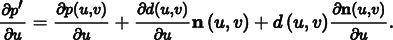
We already have computed the value of ∂p(u, v)/∂u; it’s ∂p/∂u and is available in the SurfaceInteraction structure, which also stores the surface normal n(u, v) and the partial derivative ∂n(u, v)/∂u = ∂n/∂u. The displacement function d(u, v) can be evaluated as needed, which leaves ∂d(u, v)/∂u as the only remaining term.
There are two possible approaches to finding the values of ∂d(u, v)/∂u and ∂d(u, v)/∂v. One option would be to augment the Texture interface with a method to compute partial derivatives of the underlying texture function. For example, for image map textures mapped to the surface directly using its (u, v) parameterization, these partial derivatives can be computed by subtracting adjacent texels in the u and v directions. However, this approach is difficult to extend to complex procedural textures like some of the ones defined in Chapter 10. Therefore, pbrt directly computes these values with forward differencing in the Material::Bump() method, without modifying the Texture interface. Recall the definition of the partial derivative:
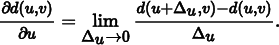
Forward differencing approximates the value using a finite value of Δu and evaluating d(u, v) at two positions. Thus, the final expression for ∂p′/∂u is the following (for simplicity, we have dropped the explicit dependence on (u, v) for some of the terms):

Interestingly enough, most bump-mapping implementations ignore the final term under the assumption that d(u, v) is expected to be relatively small. (Since bump mapping is mostly useful for approximating small perturbations, this is a reasonable assumption.) The fact that many renderers do not compute the values ∂n/∂u and ∂n/∂v may also have something to do with this simplification. An implication of ignoring the last term is that the magnitude of the displacement function then does not affect the bump-mapped partial derivatives; adding a constant value to it globally doesn’t affect the final result, since only differences of the bump function affect it. pbrt computes all three terms since it has ∂n/∂u and ∂n/∂v readily available, although in practice this final term rarely makes a visually noticeable difference.
One important detail in the definition of Bump() is that the d parameter is declared to be of type const shared_ptr < Texture < Float > > &, rather than, for example, shared_ ptr < Texture < Float > > . This difference is very important for performance, but the reason is subtle. If a C++ reference was not used here, then the shared_ptr implementation would need to increment the reference count for the temporary value passed to the method, and the reference count would need to be decremented when the method returned. This is an efficient operation with serial code, but with multiple threads of execution, it leads to a situation where multiple processing cores end up modifying the same memory location whenever different rendering tasks run this method with the same displacement texture. This state of affairs in turn leads to the expensive “read for ownership” operation described in Section A.6.1.2
〈Material Method Definitions〉 ≡
void Material::Bump(const std::shared_ptr < Texture < Float > > &d,
SurfaceInteraction *si) {
〈Compute offset positions and evaluate displacement texture 590〉
〈Compute bump-mapped differential geometry 590〉
}
〈Compute offset positions and evaluate displacement texture〉 ≡ 589
SurfaceInteraction siEval = *si;
〈Shift siEval du in the u direction 590〉
Float uDisplace = d- > Evaluate(siEval);
〈Shift siEval dv in the v direction〉
Float vDisplace = d- > Evaluate(siEval);
Float displace = d- > Evaluate(*si);
One remaining issue is how to choose the offsets Δu and Δv for the finite differencing computations. They should be small enough that fine changes in d(u, v) are captured but large enough so that available floating-point precision is sufficient to give a good result. Here, we will choose Δu and Δv values that lead to an offset that is about half the image space pixel sample spacing and use them to update the appropriate member variables in the SurfaceInteraction to reflect a shift to the offset position. (See Section 10.1.1 for an explanation of how the image space distances are computed.)
Another detail to note in the following code: we recompute the surface normal n as the cross product of ∂p/∂u and ∂p/∂v rather than using si- > shading.n directly. The reason for this is that the orientation of n may have been flipped (recall the fragment 〈Adjust normal based on orientation and handedness〉 in Section 2.10.1). However, we need the original normal here. Later, when the results of the computation are passed to SurfaceInteraction::SetShadingGeometry(), the normal we compute will itself be flipped if necessary.
〈Shift siEval du in the u direction〉 ≡ 590
Float du = .5f * (std::abs(si- > dudx) + std::abs(si- > dudy));
if (du == 0) du = .01f;
siEval.p = si- > p + du * si- > shading.dpdu;
siEval.uv = si- > uv + Vector2f(du, 0.f);
siEval.n = Normalize((Normal3f)Cross(si- > shading.dpdu,
si- > shading.dpdv) +
du * si- > dndu);
The 〈Shift siEval dv in the v direction〉 fragment is nearly the same as the fragment that shifts du, so it isn’t included here.
Given the new positions and the displacement texture’s values at them, the partial derivatives can be computed directly using Equation (9.1):
〈Compute bump-mapped differential geometry〉 ≡ 589
Vector3f dpdu = si- > shading.dpdu +
(uDisplace - displace) / du * Vector3f(si- > shading.n) +
displace * Vector3f(si- > shading.dndu);
Vector3f dpdv = si- > shading.dpdv +
(vDisplace - displace) / dv * Vector3f(si- > shading.n) +
displace * Vector3f(si- > shading.dndv);
si- > SetShadingGeometry(dpdu, dpdv, si- > shading.dndu, si- > shading.dndv,
false);
Further reading
Burley’s article (2012) on a material model developed at Disney for feature films is an excellent read. It includes extensive discussion of features of real-world reflection functions that can be observed in Matusik et al.’s (2003b) measurements of one hundred BRDFs and analyzes the ways that existing BRDF models do and do not fit these features well. These insights are then used to develop an “artist-friendly” material model that can express a wide range of surface appearances. The model describes reflection with a single color and ten scalar parameters, all of which are in the range [0, 1] and have fairly predictable effects on the appearance of the resulting material.
Blinn (1978) invented the bump-mapping technique. Kajiya (1985) generalized the idea of bump mapping the normal to frame mapping, which also perturbs the surface’s primary tangent vector and is useful for controlling the appearance of anisotropic reflection models. Mikkelsen’s thesis (2008) carefully investigates a number of the assumptions underlying bump mapping, proposes generalizations, and addresses a number of subtleties with respect to its application to real-time rendering.
Snyder and Barr (1987) noted the light leak problem from per-vertex shading normals and proposed a number of work-arounds. The method we have used in this chapter is from Section 5.3 of Veach’s thesis (1997); it is a more robust solution than those of Snyder and Barr.
Shading normals introduce a number of subtle problems for physically based light transport algorithms that we have not addressed in this chapter. For example, they can easily lead to surfaces that reflect more energy than was incident upon them, which can wreak havoc with light transport algorithms that are designed under the assumption of energy conservation. Veach (1996) investigated this issue in depth and developed a number of solutions. Section 16.1 of this book will return to this issue.
One visual shortcoming of bump mapping is that it doesn’t naturally account for self-shadowing, where bumps cast shadows on the surface and prevent light from reaching nearby points. These shadows can have a significant impact on the appearance of rough surfaces. Max (1988) developed the horizon mapping technique, which performs a preprocess on bump maps stored in image maps to compute a term to account for this effect. This approach isn’t directly applicable to procedural textures, however. Dana et al. (1999) measured spatially varying reflection properties from real-world surfaces, including these self-shadowing effects; they convincingly demonstrate this effect’s importance for accurate image synthesis.
Another difficult issue related to bump mapping is that antialiasing bump maps that have higher frequency detail than can be represented in the image is quite difficult. In particular, it is not enough to remove high-frequency detail from the bump map function, but in general the BSDF needs to be modified to account for this detail. Fournier (1992) applied normal distribution functions to this problem, where the surface normal was generalized to represent a distribution of normal directions. Becker and Max (1993) developed algorithms for blending between bump maps and BRDFs that represented higher-frequency details. Schilling (1997, 2001) investigated this issue particularly for application to graphics hardware. More recently, effective approaches to filtering bump maps were developed by Han et al. (2007) and Olano and Baker (2010). Recent work by Dupuy et al. (2013) and Hery et al. (2014) addressed this issue by developing techniques that convert displacements into anisotropic distributions of Beckmann microfacets.
An alternative to bump mapping is displacement mapping, where the bump function is used to actually modify the surface geometry, rather than just perturbing the normal (Cook 1984; Cook, Carpenter, and Catmull 1987). Advantages of displacement mapping include geometric detail on object silhouettes and the possibility of accounting for self-shadowing. Patterson and collaborators described an innovative algorithm for displacement mapping with ray tracing where the geometry is unperturbed but the ray’s direction is modified such that the intersections that are found are the same as would be found with the displaced geometry (Patterson, Hoggar, and Logie 1991; Logie and Patterson 1994). Heidrich and Seidel (1998) developed a technique for computing direct intersections with procedurally defined displacement functions.
As computers have become faster, another viable approach for displacement mapping has been to use an implicit function to define the displaced surface and to then take steps along rays until they find a zero crossing with the implicit function. At this point, an intersection has been found. This approach was first introduced by Hart (1996); see Donnelly (2005) for information about using this approach for displacement mapping on the GPU. This approach was recently popularized by Quilez on the shadertoy Web site (Quilez 2015).
With the advent of increased memory on computers and caching algorithms, the option of finely tessellating geometry and displacing its vertices for ray tracing has become feasible. Pharr and Hanrahan (1996) described an approach to this problem based on geometry caching, and Wang et al. (2000) described an adaptive tessellation algorithm that reduces memory requirements. Smits, Shirley, and Stark (2000) lazily tessellate individual triangles, saving a substantial amount of memory.
Measuring fine-scale surface geometry of real surfaces to acquire bump or displacement maps can be challenging. Johnson et al. (2011) developed a novel hand-held system that can measure detail down to a few microns, which more than suffices for these uses.
Exercises
 9.1 If the same Texture is bound to more than one component of a Material (e.g., to both PlasticMaterial::Kd and PlasticMaterial::Ks), the texture will be evaluated twice. This unnecessarily duplicated work may lead to a noticeable increase in rendering time if the Texture is itself computationally expensive. Modify the materials in pbrt to eliminate this problem. Measure the change in the system’s performance, both for standard scenes as well as for contrived scenes that exhibit this redundancy.
9.2 Implement the artist-friendly “Disney BRDF” described by Burley (2012). You will need both a new Material implementation as well as a few new BxDFs. Render a variety of scenes using your implementation. How easy do you find it to match the visual appearance of existing pbrt scenes when replacing Materials in them with this one? How quickly can you dial in the parameters of this material to achieve a given desired appearance?
 9.3 One form of aliasing that pbrt doesn’t try to eliminate is specular highlight aliasing. Glossy specular surfaces with high specular exponents, particularly if they have high curvature, are susceptible to aliasing as small changes in incident direction or surface position (and thus surface normal) may cause the highlight’s contribution to change substantially. Read Amanatides’s paper on this topic (Amanatides 1992) and extend pbrt to reduce specular aliasing, either using his technique or by developing your own. Most of the quantities needed to do the appropriate computations are already available—∂n/∂x and ∂n/∂y in the SurfaceInteraction, and so on—although it will probably be necessary to extend the BxDF interface to provide more information about the roughness of any MicrofacetDistributions they have.
9.4 Another approach to addressing specular highlight aliasing is to supersample the BSDF, evaluating it multiple times around the point being shaded. After reading the discussion of supersampling texture functions in Section 10.1, modify the BSDF::f() method to shift to a set of positions around the intersection point but within the pixel sampling rate around the intersection point and evaluate the BSDF at each one of them when the BSDF evaluation routines are called. (Be sure to account for the change in normal using its partial derivatives.) How well does this approach combat specular highlight aliasing?
9.5 Read some of the papers on filtering bump maps referenced in the “Further Reading” section of this chapter, choose one of the techniques described there, and implement it in pbrt. Show both the visual artifacts from bump map aliasing without the technique you implement as well as examples of how well your implementation addresses them.
9.6 Neyret (1996, 1998), Heitz and Neyret (2012), and Heitz et al. (2015) developed algorithms that take descriptions of complex shapes and their reflective properties and turn them into generalized reflection models at different resolutions, each with limited frequency content. The advantage of this representation is that it makes it easy to select an appropriate level of detail for an object based on its size on the screen, thus reducing aliasing. Read these papers and implement the algorithms described in them in pbrt. Show how they can be used to reduce geometric aliasing from detailed geometry, and extend them to address bump map aliasing.
9.7 Use the triangular face refinement infrastructure from the Loop subdivision surface implementation in Section 3.8 to implement displacement mapping in pbrt. The usual approach to displacement mapping is to finely tessellate the geometric shape and then to evaluate the displacement function at its vertices, moving each vertex the given distance along its normal.
Refine each face of the mesh until, when projected onto the image, it is roughly the size of the separation between pixels. To do this, you will need to be able to estimate the image pixel-based length of an edge in the scene when it is projected onto the screen. Use the texturing infrastructure in Chapter 10 to evaluate displacement functions. See Patney et al. (2009) and Fisher et al. (2009) for discussion of issues related to avoiding cracks in the mesh due to adaptive tessellation.