Volume Scattering
So far, we have assumed that scenes are made up of collections of surfaces in a vacuum, which means that radiance is constant along rays between surfaces. However, there are many real-world situations where this assumption is inaccurate: fog and smoke attenuate and scatter light, and scattering from particles in the atmosphere makes the sky blue and sunsets red. This chapter introduces the mathematics to describe how light is affected as it passes through participating media—large numbers of very small particles distributed throughout a region of 3D space. Volume scattering models are based on the assumption that there are so many particles that scattering is best modeled as a probabilistic process, rather than directly accounting for individual interactions with particles. Simulating the effect of participating media makes it possible to render images with atmospheric haze, beams of light through clouds, light passing through cloudy water, and subsurface scattering, where light exits a solid object at a different place than where it entered.
This chapter first describes the basic physical processes that affect the radiance along rays passing through participating media. It then introduces the Medium base class, which provides interfaces for describing participating media in a region of space. Medium implementations return information about the scattering properties at points in their extent, including a phase function, which characterizes how light is scattered at a point in space. (It’s the volumetric analog to the BSDF, which describes scattering at a point on a surface.) In order to determine the effect of participating media on the distribution of radiance in the scene, Integrators that handle volumetric effects are necessary; this is the topic of Chapter 15.
In highly scattering participating media, light can undergo many scattering events without any appreciable reduction in its energy. The cost of finding a light path in an Integrator is generally proportional to its length, and tracking paths with hundreds or thousands of scattering interactions quickly becomes impractical. In such cases, it is preferable to aggregate the overall effect of the underlying scattering process in a function that relates scattering between points where light enters and leaves the medium. The chapter therefore concludes with the BSSRDF base class, which is an abstraction that makes it possible to implement this type of approach. BSSRDF implementations describe the internal scattering in a medium bounded by refractive surfaces.
11.1 Volume scattering processes
There are three main processes that affect the distribution of radiance in an environment with participating media:
• Absorption: the reduction in radiance due to the conversion of light to another form of energy, such as heat
• Emission: radiance that is added to the environment from luminous particles
• Scattering: radiance heading in one direction that is scattered to other directions due to collisions with particles
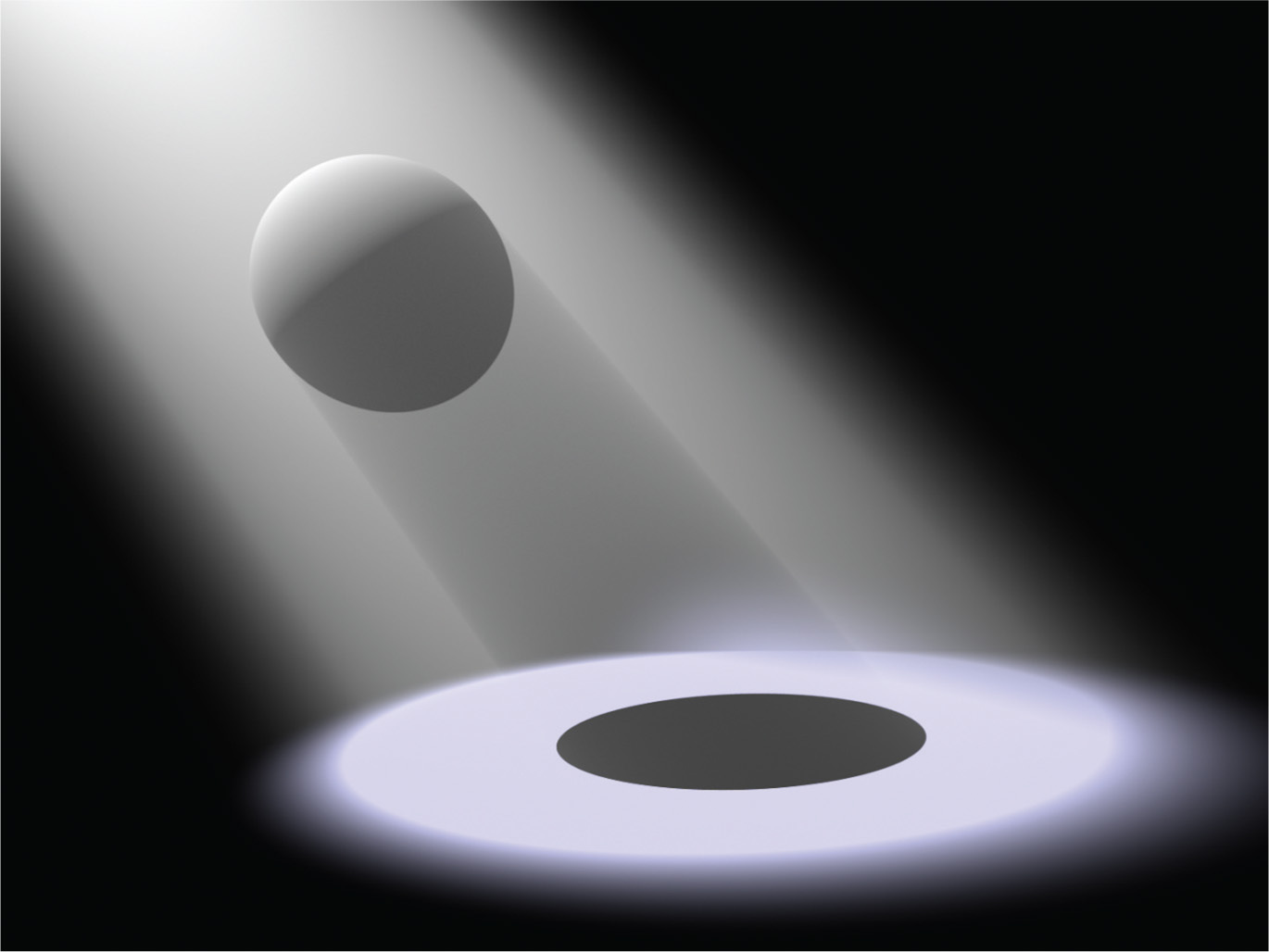
The characteristics of all of these properties may be homogeneous or inhomogeneous. Homogeneous properties are constant throughout some region of space given spatial extent, while inhomogeneous properties vary throughout space. Figure 11.1 shows a simple example of volume scattering, where a spotlight shining through a participating medium illuminates particles in the medium and casts a volumetric shadow.
11.1.1 Absorption
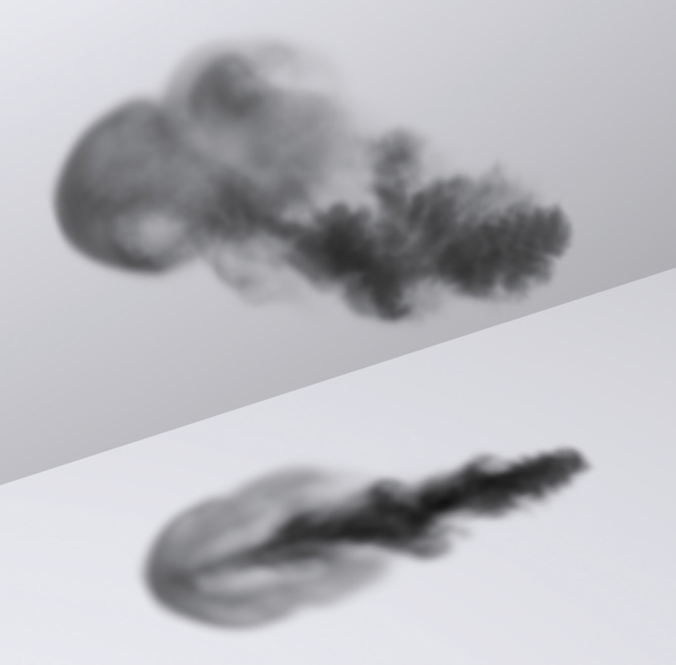
Consider thick black smoke from a fire: the smoke obscures the objects behind it because its particles absorb light traveling from the object to the viewer. The thicker the smoke, the more light is absorbed. Figure 11.2 shows this effect with a spatial distribution of absorption that was created with an accurate physical simulation of smoke formation. Note the shadow on the ground: the participating medium has also absorbed light between the light source to the ground plane, casting a shadow.
Absorption is described by the medium’s absorption cross section, σa, which is the probability density that light is absorbed per unit distance traveled in the medium. In general, the absorption cross section may vary with both position p and direction ω, although it is normally just a function of position. It is usually also a spectrally varying quantity. The units of σa are reciprocal distance (m− 1). This means that σa can take on any positive value; it is not required to be between 0 and 1, for instance.
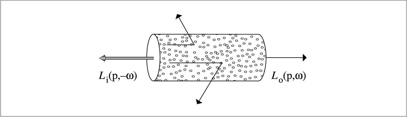
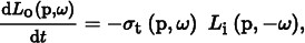
Figure 11.3 shows the effect of absorption along a very short segment of a ray. Some amount of radiance Li(p, − ω) is arriving at point p, and we’d like to find the exitant radiance Lo(p, ω) after absorption in the differential volume. This change in radiance along the differential ray length dt is described by the differential equation


which says that the differential reduction in radiance along the beam is a linear function of its initial radiance.1
This differential equation can be solved to give the integral equation describing the total fraction of light absorbed for a ray. If we assume that the ray travels a distance d in direction ω through the medium starting at point p, the remaining portion of the original radiance is given by

11.1.2 Emission
While absorption reduces the amount of radiance along a ray as it passes through a medium, emission increases it, due to chemical, thermal, or nuclear processes that convert energy into visible light. Figure 11.4 shows emission in a differential volume, where we denote emitted radiance added to a ray per unit distance at a point p in direction ω by Le(p, ω). Figure 11.5 shows the effect of emission with the smoke data set. In that figure the absorption coefficient is much lower than in Figure 11.2, giving a very different appearance.


The differential equation that gives the change in radiance due to emission is

This equation incorporates the assumption that the emitted light Le is not dependent on the incoming light Li. This is always true under the linear optics assumptions that pbrt is based on.
11.1.3 Out-scattering and attenuation
The third basic light interaction in participating media is scattering. As a ray passes through a medium, it may collide with particles and be scattered in different directions. This has two effects on the total radiance that the beam carries. It reduces the radiance exiting a differential region of the beam because some of it is deflected to different directions. This effect is called out-scattering (Figure 11.6) and is the topic of this section. However, radiance from other rays may be scattered into the path of the current ray; this in-scattering process is the subject of the next section.
The probability of an out-scattering event occurring per unit distance is given by the scattering coefficient, σs. As with absorption, the reduction in radiance along a differential length dt due to out-scattering is given by

The total reduction in radiance due to absorption and out-scattering is given by the sum σa + σs. This combined effect of absorption and out-scattering is called attenuation or extinction. For convenience the sum of these two coefficients is denoted by the attenuation coefficient σt:

Two values related to the attenuation coefficient will be useful in the following. The first is the albedo, which is defined as

The albedo is always between 0 and 1; it describes the probability of scattering (versus absorption) at a scattering event. The second is the mean free path, 1/σt, which gives the average distance that a ray travels in the medium before interacting with a particle.
Given the attenuation coefficient σt, the differential equation describing overall attenuation,
can be solved to find the beam transmittance, which gives the fraction of radiance that is transmitted between two points:
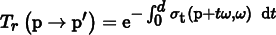
where d = ||p − p′|| is the distance between p and p′, ω is the normalized direction vector between them, and Tr denotes the beam transmittance between p and p′. Note that the transmittance is always between 0 and 1. Thus, if exitant radiance from a point p on a surface in a given direction ω is given by Lo(p, ω), after accounting for extinction, the incident radiance at another point p′ in direction − ω is
This idea is illustrated in Figure 11.7.

Two useful properties of beam transmittance are that transmittance from a point to itself is 1, Tr (p → p) = 1, and in a vacuum σt = 0 and so Tr (p → p′) = 1 for all p′. Furthermore, if the attenuation coefficient satisfies the directional symmetry σt(ω) = σt(− ω) or does not vary with direction ω and only varies as function of position (this is generally the case), then the transmittance between two points is the same in both directions:
This property follows directly from Equation (11.1).
Another important property, true in all media, is that transmittance is multiplicative along points on a ray:

for all points p′ between p and p″ (Figure 11.8). This property is useful for volume scattering implementations, since it makes it possible to incrementally compute transmittance at multiple points along a ray: transmittance from the origin to a point Tr (o → p) can be computed by taking the product of transmittance to a previous point Tr (o → p′) and the transmittance of the segment between the previous and the current point Tr (p′ → p).

The negated exponent in the definition of Tr in Equation (11.1) is called the optical thickness between the two points. It is denoted by the symbol τ :

In a homogeneous medium, σt is a constant, so the integral that defines τ is trivially evaluated, giving Beer’s law:
11.1.4 In-scattering
While out-scattering reduces radiance along a ray due to scattering in different directions, in-scattering accounts for increased radiance due to scattering from other directions (Figure 11.9). Figure 11.10 shows the effect of in-scattering with the smoke data set. Note that the smoke appears much thicker than when absorption or emission was the dominant volumetric effect.


Assuming that the separation between particles is at least a few times the lengths of their radii, it is possible to ignore inter-particle interactions when describing scattering at a particular location. Under this assumption, the phase function p(ω, ω′) describes the angular distribution of scattered radiation at a point; it is the volumetric analog to the BSDF. The BSDF analogy is not exact, however. For example, phase functions have a normalization constraint: for all ω, the condition
must hold. This constraint means that phase functions actually define probability distributions for scattering in a particular direction.
The total added radiance per unit distance due to in-scattering is given by the source term Ls:

It accounts for both volume emission and in-scattering:

The in-scattering portion of the source term is the product of the scattering probability per unit distance, σs, and the amount of added radiance at a point, which is given by the spherical integral of the product of incident radiance and the phase function. Note that the source term is very similar to the scattering equation, Equation (5.9); the main difference is that there is no cosine term since the phase function operates on radiance rather than differential irradiance.
11.2 Phase functions
Just as there is a wide variety of BSDF models that describe scattering from surfaces, many phase functions have also been developed. These range from parameterized models (which can be used to fit a function with a small number of parameters to measured data) to analytic models that are based on deriving the scattered radiance distribution that results from particles with known shape and material (e.g., spherical water droplets).
In most naturally occurring media, the phase function is a 1D function of the angle θ between the two directions ωo and ωi; these phase functions are often written as p(cos θ). Media with this type of phase function are called isotropic because their response to incident illumination is (locally) invariant under rotations. In addition to being normalized, an important property of naturally occurring phase functions is that they are reciprocal: the two directions can be interchanged and the phase function’s value remains unchanged. Note that isotropic phase functions are trivially reciprocal because cos(− θ) = cos(θ).
In anisotropic media that consist of particles arranged in a coherent structure, the phase function can be a 4D function of the two directions, which satisfies a more involved kind of reciprocity relation. Examples of this are crystals or media made of coherently oriented fibers; the “Further Reading” discusses these types of media further.
In a slightly confusing overloading of terminology, phase functions themselves can be isotropic or anisotropic as well. Thus, we might have an anisotropic phase function in an isotropic medium. An isotropic phase function describes equal scattering in all directions and is thus independent of either of the two directions. Because phase functions are normalized, there is only one such function:
The PhaseFunction abstract base class defines the interface for phase functions in pbrt.
〈Media Declarations〉 ≡
class PhaseFunction {
public:
〈PhaseFunction Interface 681〉
};
The p() method returns the value of the phase function for the given pair of directions. As with BSDFs, pbrt uses the convention that the two directions both point away from the point where scattering occurs; this is a different convention from what is usually used in the scattering literature (Figure 11.11).

〈PhaseFunction Interface〉 ≡ 681
virtual Float p(const Vector3f &wo, const Vector3f &wi) const = 0;
A widely used phase function was developed by Henyey and Greenstein (1941). This phase function was specifically designed to be easy to fit to measured scattering data. A single parameter g (called the asymmetry parameter) controls the distribution of scattered light2:
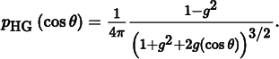
The PhaseHG() function implements this computation.
〈Media Inline Functions〉 ≡
inline Float PhaseHG(Float cosTheta, Float g) {
Float denom = 1 + g * g + 2 * g * cosTheta;
return Inv4Pi * (1 - g * g) / (denom * std::sqrt(denom));
}
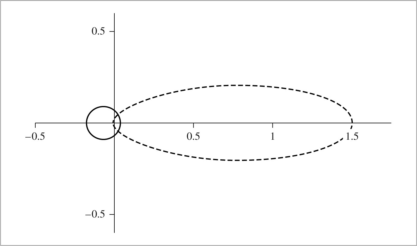
Figure 11.12 shows plots of the Henyey–Greenstein phase function with varying asymmetry parameters. The value of g for this model must be in the range (− 1, 1). Negative values of g correspond to back-scattering, where light is mostly scattered back toward the incident direction, and positive values correspond to forward-scattering. The greater the magnitude of g, the more scattering occurs close to the ω or − ω directions (for backscattering and forward-scattering, respectively). See Figure 11.13 to compare the visual effect of forward- and back-scattering.

HenyeyGreenstein provides a PhaseFunction implementation of the Henyey–Greenstein model.
〈HenyeyGreenstein Declarations〉 ≡
class HenyeyGreenstein : public PhaseFunction {
public:
〈HenyeyGreenstein Public Methods 682〉
private:
const Float g;
};
〈HenyeyGreenstein Public Methods〉 ≡ 682
HenyeyGreenstein(Float g) : g(g) { }
〈HenyeyGreenstein Method Definitions〉 ≡
Float HenyeyGreenstein::p(const Vector3f &wo, const Vector3f &wi) const {
return PhaseHG(Dot(wo, wi), g);
}
The asymmetry parameter g in the Henyey–Greenstein model has a precise meaning. It is the average value of the product of the phase function being approximated and the cosine of the angle between ω′ and ω. Given an arbitrary phase function p, the value of g can be computed as3

Thus, an isotropic phase function gives g = 0, as expected.
Any number of phase functions can satisfy this equation; the g value alone is not enough to uniquely describe a scattering distribution. Nevertheless, the convenience of being able to easily convert a complex scattering distribution into a simple parameterized model is often more important than this potential loss in accuracy.
More complex phase functions that aren’t described well with a single asymmetry parameter can often be modeled by a weighted sum of phase functions like Henyey–Greenstein, each with different parameter values:

where the weights wi sum to one to maintain normalization. This generalization isn’t provided in pbrt but would be easy to add.
11.3 Media
Implementations of the Medium base class provide various representations of volumetric scattering properties in a region of space. In a complex scene, there may be multiple Medium instances, each representing a different scattering effect. For example, an outdoor lake scene might have one Medium to model atmospheric scattering, another to model mist rising from the lake, and a third to model particles suspended in the water of the lake.
〈Medium Declarations〉 ≡
class Medium {
public:
〈Medium Interface 684〉
};
A key operation that Medium implementations must perform is to compute the beam transmittance, Equation (11.1), along a given ray passed to its Tr() method. Specifically, the method should return an estimate of the transmittance on the interval between the ray origin and the point at a distance of Ray::tMax from the origin.
Medium-aware Integrators using this interface are responsible for accounting for interactions with surfaces in the scene as well as the spatial extent of the Medium; hence we will assume that the ray passed to the Tr() method is both unoccluded and fully contained within the current Medium. Some implementations of this method use Monte Carlo integration to compute the transmittance; a Sampler is provided for this case. (See Section 15.2.)
〈Medium Interface〉 ≡ 684
virtual Spectrum Tr(const Ray &ray, Sampler &sampler) const = 0;
The spatial distribution and extent of media in a scene is defined by associating Medium instances with the camera, lights, and primitives in the scene. For example, Cameras store a Medium pointer that gives the medium for rays leaving the camera and similarly for Lights.
In pbrt, the boundary between two different types of scattering media is always represented by the surface of a GeometricPrimitive. Rather than storing a single Medium pointer like lights and cameras, GeometricPrimitives hold a MediumInterface, which in turn holds pointers to one Medium for the interior of the primitive and one for the exterior. For all of these cases, a nullptr can be used to indicate a vacuum (where no volumetric scattering occurs.)
〈MediumInterface Declarations〉 ≡
struct MediumInterface {
〈MediumInterface Public Methods 685〉
const Medium *inside, *outside;
};
This approach to specifying the extent of participating media does allow the user to specify impossible or inconsistent configurations. For example, a primitive could be specified as having one medium outside of it, and the camera could be specified as being in a different medium without a MediumInterface between the camera and the surface of the primitive. In this case, a ray leaving the primitive toward the camera would be treated as being in a different medium from a ray leaving the camera toward the primitive. In turn, light transport algorithms would be unable to compute consistent results. For pbrt’s purposes, we think it’s reasonable to expect that the user will be able to specify a consistent configuration of media in the scene and that the added complexity of code to check this isn’t worthwhile.
A MediumInterface can be initialized with either one or two Medium pointers. If only one is provided, then it represents an interface with the same medium on both sides.
〈MediumInterface Public Methods〉 ≡ 684
MediumInterface(const Medium *medium)
: inside(medium), outside(medium) { }
MediumInterface(const Medium *inside, const Medium *outside)
: inside(inside), outside(outside) { }
The function MediumInterface::IsMediumTransition() checks whether a particular MediumInterface instance marks a transition between two distinct media.
〈MediumInterface Public Methods〉 + ≡ 684
bool IsMediumTransition() const { return inside ! = outside; }
We can now provide a missing piece in the implementation of the GeometricPrimitive:: Intersect() method. The code in this fragment is executed whenever an intersection with a geometric primitive has been found; its job is to set the medium interface at the intersection point.
Instead of simply copying the value of the GeometricPrimitive::mediumInterface field, we will follow a slightly different approach and only use this information when this MediumInterface specifies a proper transition between participating media. Otherwise, the Ray::medium field takes precedence.
Setting the SurfaceInteraction’s mediumInterface field in this way greatly simplifies the specification of scenes containing media: in particular, it is not necessary to tag every scene surface that is in contact with a medium. Instead, only non-opaque surfaces that have different media on each side require an explicit medium reference in their GeometricPrimitive::mediumInterface field. In the simplest case where a scene containing opaque objects is filled with a participating medium (e.g., haze), it is enough to tag the camera and light sources.
〈Initialize SurfaceInteraction::mediumInterface after Shape intersection〉 ≡ 251
if (mediumInterface.IsMediumTransition())
isect- > mediumInterface = mediumInterface;
else
isect- > mediumInterface = MediumInterface(r.medium);
Primitives associated with shapes that represent medium boundaries generally have a Material associated with them. For example, the surface of a lake might use an instance of GlassMaterial to describe scattering at the lake surface, which also acts as the boundary between the rising mist’s Medium and the lake water’s Medium. However, sometimes we only need the shape for the boundary surface it provides to delimit a participating medium boundary and we don’t want to see the surface itself. For example, the medium representing a cloud might be bounded by a box made of triangles where the triangles are only there to delimit the cloud’s extent and shouldn’t otherwise affect light passing through them.
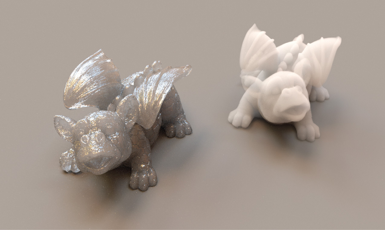
While such a surface that disappears and doesn’t affect ray paths could be perfectly accurately described by a BTDF that represented perfect specular transmission with the same index of refraction on both sides, dealing with such surfaces places extra burden on the Integrators (not all of which handle this type of specular light transport well). Therefore, pbrt allows such surfaces to have a Material * that is nullptr, indicating that they do not affect light passing through them; in turn, SurfaceInteraction::bsdf will also be nullptr, and the light transport routines don’t worry about light scattering from such surfaces and only account for changes in the current medium at them. Figure 11.14 has two instances of the dragon model filled with scattering media; one has a scattering surface at the boundary and the other does not.
Given these conventions for how Medium implementations are associated with rays passing through regions of space, we will implement a Scene::IntersectTr() method, which is a generalization of Scene::Intersect() that returns the first intersection with a light-scattering surface along the given ray as well as the beam transmittance up to that point. (If no intersection is found, this method returns false and doesn’t initialize the provided SurfaceInteraction.)
〈Scene Method Definitions〉 + ≡
bool Scene::IntersectTr(Ray ray, Sampler &sampler,
SurfaceInteraction *isect, Spectrum *Tr) const {
*Tr = Spectrum(1.f);
while (true) {
bool hitSurface = Intersect(ray, isect);
〈Accumulate beam transmittance for ray segment 687〉
〈Initialize next ray segment or terminate transmittance computation 687〉
}
}
Each time through the loop, the transmittance along the ray is accumulated into the overall beam transmittance *Tr. Recall that Scene::Intersect() will have updated the ray’s tMax member variable to the intersection point if it did intersect a surface. The Tr() implementation will use this value to find the segment over which to compute transmittance.
〈Accumulate beam transmittance for ray segment〉 ≡ 687
if (ray.medium)
*Tr * = ray.medium- > Tr(ray, sampler);
The loop ends when no intersection is found or when a scattering surface is intersected. If an optically inactive surface with its bsdf equal to nullptr is intersected, a new ray is spawned in the same direction from the intersection point, though potentially in a different medium, based on the intersection’s MediumInterface field.4
〈Initialize next ray segment or terminate transmittance computation〉 ≡ 687
if (!hitSurface)
return false;
if (isect- > primitive- > GetMaterial() ! = nullptr)
return true;
ray = isect- > SpawnRay(ray.d);
11.3.1 Medium interactions
Section 2.10 introduced the general Interaction class as well as the SurfaceInteraction specialization to represent interactions at surfaces. Now that we have some machinery for describing scattering in volumes, it’s worth generalizing these representations. First, we’ll add two more Interaction constructors for interactions at points in scattering media.
〈Interaction Public Methods〉 + ≡ 115
Interaction(const Point3f &p, const Vector3f &wo, Float time,
const MediumInterface &mediumInterface)
: p(p), time(time), wo(wo), mediumInterface(mediumInterface) { }
〈Interaction Public Methods〉 + ≡ 115
Interaction(const Point3f &p, Float time,
const MediumInterface &mediumInterface)
: p(p), time(time), mediumInterface(mediumInterface) { }
〈Interaction Public Methods〉 + ≡ 115
bool IsMediumInteraction() const { return !IsSurfaceInteraction(); }
For surface interactions where Interaction::n has been set, the Medium * for a ray leaving the surface in the direction w is returned by the GetMedium() method.
〈Interaction Public Methods〉 + ≡ 115
const Medium *GetMedium(const Vector3f &w) const {
return Dot(w, n) > 0 ? mediumInterface.outside :
mediumInterface.inside;
}
For interactions that are known to be inside participating media, another variant of GetMedium() that doesn’t take the unnecessary outgoing direction vector returns the Medium *.
〈Interaction Public Methods〉 + ≡ 115
const Medium *GetMedium() const {
Assert(mediumInterface.inside == mediumInterface.outside);
return mediumInterface.inside;
}
Just as the SurfaceInteraction class represents an interaction obtained by intersecting a ray against the scene geometry, MediumInteraction represents an interaction at a point in a scattering medium that is obtained using a similar kind of operation.
〈Interaction Declarations〉 + ≡
class MediumInteraction : public Interaction {
public:
〈MediumInteraction Public Methods 688〉
〈MediumInteraction Public Data 688〉
};
〈MediumInteraction Public Methods〉 ≡ 688
MediumInteraction(const Point3f &p, const Vector3f &wo, Float time,
const Medium *medium, const PhaseFunction *phase)
: Interaction(p, wo, time, medium), phase(phase) { }
MediumInteraction adds a new PhaseFunction member variable to store the phase function associated with its position.
〈MediumInteraction Public Data〉 ≡ 688
const PhaseFunction *phase;
11.3.2 Homogeneous medium
The HomogeneousMedium is the simplest possible medium; it represents a region of space with constant σa and σs values throughout its extent. It uses the Henyey–Greenstein phase function to represent scattering in the medium, also with a constant g value. This medium was used for the images in Figure 11.13 and 11.14.
〈HomogeneousMedium Declarations〉 ≡
class HomogeneousMedium : public Medium {
public:
〈HomogeneousMedium Public Methods 689〉
private:
〈HomogeneousMedium Private Data 689〉
};
〈HomogeneousMedium Public Methods〉 ≡ 689
HomogeneousMedium(const Spectrum &sigma_a, const Spectrum &sigma_s,
Float g)
: sigma_a(sigma_a), sigma_s(sigma_s), sigma_t(sigma_s + sigma_a),
g(g) { }
〈HomogeneousMedium Private Data〉 ≡ 689
const Spectrum sigma_a, sigma_s, sigma_t;
const Float g;
Because σt is constant throughout the medium, Beer’s law, Equation (11.3), can be used to compute transmittance along the ray. However, implementation of the Tr() method is complicated by some subtleties of floating-point arithmetic. As discussed in Section 3.9.1, IEEE floating point provides a representation for infinity; in pbrt, this value, Infinity, is used to initialize Ray::tMax for rays leaving cameras and lights, which is useful for ray–intersection tests in that it ensures that any actual intersection, even if far along the ray, is detected as an intersection for a ray that hasn’t intersected anything yet.
However, the use of Infinity for Ray::tMax creates a small problem when applying Beer’s law. In principle, we just need to compute the parametric t range that the ray spans, multiply by the ray direction’s length, and then multiply by σt:
Float d = ray.tMax * ray.Length();
Spectrum tau = sigma_t * d;
return Exp(-tau);
The problem is that multiplying Infinity by zero results in the floating-point “not a number” (NaN) value, which propagates throughout all computations that use it. For a ray that passes infinitely far through a medium with zero absorption for a given spectral channel, the above code would attempt to perform the multiplication 0 * Infinity and would produce a NaN value rather than the expected transmittance of zero. The implementation here resolves this issue by clamping the ray segment length to the largest representable non-infinite floating-point value.
〈HomogeneousMedium Method Definitions〉 ≡
Spectrum HomogeneousMedium::Tr(const Ray &ray, Sampler &sampler) const {
return Exp(-sigma_t * std::min(ray.tMax * ray.d.Length(), MaxFloat));
}
11.3.3 3d grids
The GridDensityMedium class stores medium densities at a regular 3D grid of positions, similar to the way that the ImageTexture represents images with a 2D grid of samples. These samples are interpolated to compute the density at positions between the sample points. The implementation of the GridDensityMedium is in media/grid.h and media/grid.cpp.
〈GridDensityMedium Declarations〉 ≡
class GridDensityMedium : public Medium {
public:
〈GridDensityMedium Public Methods 690〉
private:
〈GridDensityMedium Private Data 690〉
};
The constructor takes a 3D array of user-supplied density values, thus allowing a variety of sources of data (physical simulation, CT scan, etc.). The smoke data set rendered in Figures 11.2, 11.5, and 11.10 is represented with a GridDensityMedium. The caller also supplies baseline values of σa, σs, and g to the constructor, which does the usual initialization of the basic scattering properties and makes a local copy of the density values.
〈GridDensityMedium Public Methods〉 ≡ 690
GridDensityMedium(const Spectrum &sigma_a, const Spectrum &sigma_s,
Float g, int nx, int ny, int nz, const Transform &mediumToWorld,
const Float *d)
: sigma_a(sigma_a), sigma_s(sigma_s), g(g), nx(nx), ny(ny), nz(nz),
WorldToMedium(Inverse(mediumToWorld)),
density(new Float[nx * ny * nz]) {
memcpy((Float *)density.get(), d, sizeof(Float) * nx * ny * nz);
〈Precompute values for Monte Carlo sampling of GridDensityMedium 896〉
}
〈GridDensityMedium Private Data〉 ≡ 690
const Spectrum sigma_a, sigma_s;
const Float g;
const int nx, ny, nz;
const Transform WorldToMedium;
std::unique_ptr < Float[] > density;
The Density() method of GridDensityMedium is called by GridDensityMedium::Tr(); it uses the provided samples to reconstruct the volume density function at the given point, which will already have been transformed into local coordinates using WorldToMedium. In turn, σa and σs will be scaled by the interpolated density at the point.
〈GridDensityMedium Method Definitions〉 ≡
Float GridDensityMedium::Density(const Point3f &p) const {
〈Compute voxel coordinates and offsets for p 691〉
〈Trilinearly interpolate density values to compute local density 691〉
}
The grid samples are assumed to be over a canonical [0, 1]3 domain. (The WorldToMedium transformation should be used to place the GridDensityMedium in the scene.) To interpolate the samples around a point, the Density() method first computes the coordinates of the point with respect to the sample coordinates and the distances from the point to the samples below it (along the lines of what was done in the Film and MIPMap —see also Section 7.1.7).
〈Compute voxel coordinates and offsets for p〉 ≡ 691
Point3f pSamples(p.x * nx - .5f, p.y * ny - .5f, p.z * nz - .5f);
Point3i pi = (Point3i)Floor(pSamples);
Vector3f d = pSamples - (Point3f)pi;
The distances d can be used directly in a series of invocations of Lerp() to trilinearly interpolate the density at the sample point:
〈Trilinearly interpolate density values to compute local density〉 ≡ 691
Float d00 = Lerp(d.x, D(pi), D(pi + Vector3i(1,0,0)));
Float d10 = Lerp(d.x, D(pi + Vector3i(0,1,0)), D(pi + Vector3i(1,1,0)));
Float d01 = Lerp(d.x, D(pi + Vector3i(0,0,1)), D(pi + Vector3i(1,0,1)));
Float d11 = Lerp(d.x, D(pi + Vector3i(0,1,1)), D(pi + Vector3i(1,1,1)));
Float d0 = Lerp(d.y, d00, d10);
Float d1 = Lerp(d.y, d01, d11);
return Lerp(d.z, d0, d1);
The D() utility method returns the density at the given integer sample position. Its only tasks are to handle out-of-bounds sample positions and to compute the appropriate array offset for the given sample. Unlike MIPMaps, where a variety of behavior is useful in the case of out-of-bounds coordinates, here it’s reasonable to always return a zero density for them: the density is defined over a particular domain, and it’s reasonable that points outside of it should have zero density.
〈GridDensityMedium Public Methods〉 + ≡ 690
Float D(const Point3i &p) const {
Bounds3i sampleBounds(Point3i(0, 0, 0), Point3i(nx, ny, nz));
if (!InsideExclusive(p, sampleBounds))
return 0;
return density[(p.z * ny + p.y) * nx + p.x];
}
11.4 The bssrdf
The bidirectional scattering-surface reflectance distribution function (BSSRDF) was introduced in Section 5.6.2; it gives exitant radiance at a point on a surface po given incident differential irradiance at another point pi: S(po, ωo, pi, ωi). Accurately rendering translucent surfaces with subsurface scattering requires integrating over both area—points on the surface of the object being rendered—and incident direction, evaluating the BSSRDF and computing reflection with the subsurface scattering equation

Subsurface light transport is described by the volumetric scattering processes introduced in Sections 11.1 and 11.2 as well as the volume light transport equation that will be introduced in Section 15.1. The BSSRDF S is a summarized representation modeling the outcome of these scattering processes between a given pair of points and directions on the boundary.
A variety of BSSRDF models have been developed to model subsurface reflection; they generally include some simplifications to the underlying scattering processes to make them tractable. One such model will be introduced in Section 15.5. Here, we will begin by specifying a fairly abstract interface analogous to BSDF. All of the code related to BSSRDFs is in the files core/bssrdf.h and core/bssrdf.cpp.
〈BSSRDF Declarations〉 ≡
class BSSRDF {
public:
〈BSSRDF Public Methods 692〉
〈BSSRDF Interface 693〉
protected:
〈BSSRDF Protected Data 692〉
};
BSSRDF implementations must pass the current (outgoing) surface interaction as well as the index of refraction of the scattering medium to the base class constructor. There is thus an implicit assumption that the index of refraction is constant throughout the medium, which is a widely used assumption in BSSRDF models.
〈BSSRDF Public Methods〉 ≡ 692
BSSRDF(const SurfaceInteraction &po, Float eta)
: po(po), eta(eta) { }
〈BSSRDF Protected Data〉 ≡ 692
const SurfaceInteraction &po;
Float eta;
The key method that BSSRDF implementations must provide is one that evaluates the eight-dimensional distribution function S(), which quantifies the ratio of differential radiance at point po in direction ωo to the incident differential flux at pi from direction ωi (Section 5.6.2). Since the po and ωo arguments are already available via the BSSRDF::po and Interaction::wo fields, they aren’t included in the method signature.
〈BSSRDF Interface〉 ≡ 692
virtual Spectrum S(const SurfaceInteraction &pi, const Vector3f &wi) = 0;
Like the BSDF, the BSSRDF interface also defines functions to sample the distribution and to evaluate the probability density of the implemented sampling scheme. The specifics of this part of the interface are discussed in Section 15.4.
During the shading process, the current Material’s ComputeScatteringFunctions() method initializes the SurfaceInteraction::bssrdf member variable with an appropriate BSSRDF if the material exhibits subsurface scattering. (Section 11.4.3 will define two materials for subsurface scattering.)
11.4.1 Separable bssrdfs
One issue with the BSSRDF interface as defined above is its extreme generality. Finding solutions to the subsurface light transport even in simple planar or spherical geometries is already a fairly challenging problem, and the fact that BSSRDF implementations can be attached to arbitrary and considerably more complex Shapes leads to an impracticably difficult context. To retain the ability to support general Shapes, we’ll introduce a simpler BSSRDF representation in SeparableBSSRDF.
〈BSSRDF Declarations〉 + ≡
class SeparableBSSRDF : public BSSRDF {
public:
〈SeparableBSSRDF Public Methods 693〉
〈SeparableBSSRDF Interface 695〉
private:
〈SeparableBSSRDF Private Data 693〉
};
The constructor of SeparableBSSRDF initializes a local coordinate frame defined by ss, ts, and ns, records the current light transport mode mode, and keeps a pointer to the underlying Material. The need for these values will be clarified in Section 15.4.
〈SeparableBSSRDF Public Methods〉 ≡ 693
SeparableBSSRDF(const SurfaceInteraction &po, Float eta,
const Material *material, TransportMode mode)
: BSSRDF(po, eta), ns(po.shading.n), ss(Normalize(po.shading.dpdu)),
ts(Cross(ns, ss)), material(material), mode(mode) { }
〈SeparableBSSRDF Private Data〉 ≡ 693
const Normal3f ns;
const Vector3f ss, ts;
const Material *material;
const TransportMode mode;
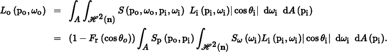
The simplified SeparableBSSRDF interface casts the BSSRDF into a separable form with three independent components (one spatial and two directional):

The Fresnel term at the beginning models the fraction of the light that is transmitted into direction ωo after exiting the material. A second Fresnel term contained inside Sω(ωi) accounts for the influence of the boundary on the directional distribution of light entering the object from direction ωi. The profile term Sp is a spatial distribution characterizing how far light travels after entering the material.
For high-albedo media, the scattered radiance distribution is generally fairly isotropic and the Fresnel transmittance is the most important factor for defining the final directional distribution. However, directional variation can be meaningful for lowalbedo media; in that case, this approximation is less accurate.
〈SeparableBSSRDF Public Methods〉 + ≡ 693
Spectrum S(const SurfaceInteraction &pi, const Vector3f &wi) {
Float Ft = 1 - FrDielectric(Dot(po.wo, po.shading.n), 1, eta);
return Ft * Sp(pi) * Sw(wi);
}
Given the separable expression in Equation (11.6), the integral for determining the outgoing illumination due to subsurface scattering (Section 15.5) simplifies to
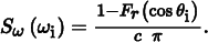
We define the directional term Sω(ωi) as a scaled version of the Fresnel transmittance (Section 8.2):
The normalization factor c is chosen so that Sω integrates to one over the cosineweighted hemisphere:

In other words,
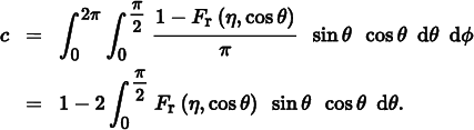
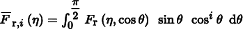
This integral is referred to as the first moment of the Fresnel reflectance function. Other moments involving higher powers of the cosine function also exist and frequently occur in subsurface scattering-related computations; the general definition of the ith Fresnel moment is
pbrt provides two functions FresnelMoment1() and FresnelMoment2() that evaluate the corresponding moments based on polynomial fits to these functions. (We won’t include their implementations in the book here.) One subtlety is that these functions follow a convention that is slightly different from the above definition—they are actually called with the reciprocal of η. This is due to their main application in Section 15.5, where they account for the effect light that is reflected back into the material due to a reflection at the internal boundary with a relative index of refraction of 1/η.
〈BSSRDF Utility Declarations〉 ≡
Float FresnelMoment1(Float invEta);
Float FresnelMoment2(Float invEta);
Using FresnelMoment1(), the definition of SeparableBSSRDF::Sw() based on Equation (11.7) can be easily implemented.
〈SeparableBSSRDF Public Methods〉 + ≡ 693
Spectrum Sw(const Vector3f &w) const {
Float c = 1 - 2 * FresnelMoment1(1 / eta);
return (1 - FrDielectric(CosTheta(w), 1, eta)) / (c * Pi);
}
Decoupling the spatial and directional arguments considerably reduces the dimension of S but does not address the fundamental difficulty with regard to supporting general Shape implementations. We introduce a second approximation, which assumes that the surface is not only locally planar but that it is the distance between the points rather than their actual locations that affects the value of the BSSRDF. This reduces Sp to a function Sr that only involves distance of the two points po and pi:

As before, the actual implementation of the spatial term Sp doesn’t take po as an argument, since it is already available in BSSRDF::po.
〈SeparableBSSRDF Public Methods〉 + ≡ 693
Spectrum Sp(const SurfaceInteraction &pi) const {
return Sr(Distance(po.p, pi.p));
}
The SeparableBSSRDF::Sr() method remains virtual—it is overridden in subclasses that implement specific 1D subsurface scattering profiles. Note that the dependence on the distance introduces an implicit assumption that the scattering medium is relatively homogeneous and does not strongly vary as a function of position—any variation should be larger than the mean free path length.
〈SeparableBSSRDF Interface〉 ≡ 693
virtual Spectrum Sr(Float d) const = 0;
BSSRDF models are usually models of the function Sr() derived through a careful analysis of the light transport within a homogeneous slab. This means models such as the SeparableBSSRDF will yield good approximations in the planar setting, but with increasing error as the underlying geometry deviates from this assumption.
11.4.2 Tabulated bssrdf
〈BSSRDF Declarations〉 + ≡
class TabulatedBSSRDF : public SeparableBSSRDF {
public:
〈TabulatedBSSRDF Public Methods 697〉
private:
〈TabulatedBSSRDF Private Data 697〉
};
The single current implementation of the SeparableBSSRDF interface in pbrt is the TabulatedBSSRDF class. It provides access to a tabulated BSSRDF representation that can handle a wide range of scattering profiles including measured real-world BSSRDFs. TabulatedBSSRDF uses the same type of adaptive spline-based interpolation method that was also used by the FourierBSDF reflectance model (Section 8.6); in this case, we are interpolating the distance-dependent scattering profile function Sr from Equation (11.9). The FourierBSDF’s second stage of capturing directional variation using Fourier series is not needed. Figure 11.15 shows spheres rendered using the TabulatedBSSRDF.

It is important to note that the radial profile Sr is only a 1D function when all BSSRDF material properties are fixed. More generally, it depends on four additional parameters: the index of refraction η, the scattering anisotropy g, the albedo ρ, and the extinction coefficient σt, leading to a complete function signature Sr(η, g, ρ, σt, r) that is unfortunately too high-dimensional for discretization. We must thus either remove or fix some of the parameters.
Consider that the only parameter with physical units (apart from r) is σt. This parameter quantifies the rate of scattering or absorption interactions per unit distance. The effect of σt is simple: it only controls the spatial scale of the BSSRDF profile. To reduce the dimension of the necessary tables, we thus fix σt = 1 and tabulate a unitless version of the BSSRDF profile.
When a lookup for a given extinction coefficient σt and radius r occurs at run time we find the corresponding unitless optical radius roptical = σtr and evaluate the lowerdimensional tabulation as follows:

Since Sr is a 2D density function in polar coordinates (r, ϕ), a corresponding scale factor of  is needed to account for this change of variables (see also Section 13.5.2).
We will also fix the index of refraction η and scattering anisotropy parameter g—in practice, this means that these parameters cannot be textured over an object that has a material that uses a TabulatedBSSRDF. These simplifications leave us with a fairly manageable 2D function that is only discretized over albedos ρ and optical radii r.
The TabulatedBSSRDF constructor takes all parameters of the BSSRDF constructor in addition to spectrally varying absorption and scattering coefficients σa and σs. It precomputes the extinction coefficient σt = σa + σs and albedo ρ = σs/σt for the current surface location, avoiding issues with a division by zero when there is no extinction for a given spectral channel.
〈TabulatedBSSRDF Public Methods〉 ≡ 696
TabulatedBSSRDF(const SurfaceInteraction &po,
const Material *material, TransportMode mode, Float eta,
const Spectrum &sigma_a, const Spectrum &sigma_s,
const BSSRDFTable &table)
: SeparableBSSRDF(po, eta, material, mode), table(table) {
sigma_t = sigma_a + sigma_s;
for (int c = 0; c < Spectrum::nSamples; ++c)
rho[c] = sigma_t[c] ! = 0 ? (sigma_s[c] / sigma_t[c]) : 0;
}
〈TabulatedBSSRDF Private Data〉 ≡ 696
const BSSRDFTable &table;
Spectrum sigma_t, rho;
Detailed information about the scattering profile Sr is supplied via the table parameter, which is an instance of the BSSRDFTable data structure:
〈BSSRDF Declarations〉 + ≡
struct BSSRDFTable {
〈BSSRDFTable Public Data 698〉
〈BSSRDFTable Public Methods 698〉
};
Instances of BSSRDFTable record samples of the function Sr taken at a set of single scattering albedos (ρ1, ρ2, …, ρn) and radii (r1, r2, …, rm). The spacing between radius and albedo samples will generally be non-uniform in order to more accurately represent the underlying function. Section 15.5.8 will show how to initialize the BSSRDFTable for a specific BSSRDF model.
We omit the constructor implementation, which takes the desired resolution and allocates memory for the representation.
〈BSSRDFTable Public Methods〉 ≡ 697
BSSRDFTable(int nRhoSamples, int nRadiusSamples);
The sample locations and counts are exposed as public member variables.
〈BSSRDFTable Public Data〉 ≡ 697
const int nRhoSamples, nRadiusSamples;
std::unique_ptr < Float[] > rhoSamples, radiusSamples;
A sample value is stored in the profile member variable for each of the m × n pairs (ρi, rj).
〈BSSRDFTable Public Data〉 + ≡ 697
std::unique_ptr < Float[] > profile;
Note that the TabulatedBSSRDF::rho member variable gives the reduction in energy after a single scattering event; this is different from the material’s overall albedo, which takes all orders of scattering into account. To stress the difference, we will refer to these different types of albedos as the single scattering albedo ρ and the effective albedo ρeff.
We define the effective albedo as the following integral of the profile Sr in polar coordinates.
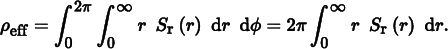
The value of ρeff will frequently be accessed both by the profile sampling code and by the KdSubsurfaceMaterial. We introduce an array rhoEff of length BSSRDFTable::nRho Samples, which maps every albedo sample to its corresponding effective albedo.
〈BSSRDFTable Public Data〉 + ≡ 697
std::unique_ptr < Float[] > rhoEff;
Computation of ρeff will be discussed in Section 15.5. For now, we only note that it is a nonlinear and strictly monotonically increasing function of the single scattering albedo ρ.
Given radius value r and single scattering albedo, the function Sr() implements a spline-interpolated lookup into the tabulated profile. The albedo parameter is taken to be the TabulatedBSSRDF::rho value. There is thus an implicit assumption that the albedo does not vary within the support of the BSSRDF profile centered around po.
Since the albedo is of type Spectrum, the function performs a separate profile lookup for each spectral channel and returns a Spectrum as a result. The return value must beclamped in case the interpolation produces slightly negative values.
〈BSSRDF Method Definitions〉 ≡
Spectrum TabulatedBSSRDF::Sr(Float r) const {
Spectrum Sr(0.f);
for (int ch = 0; ch < Spectrum::nSamples; ++ch) {
〈Convert r into unitless optical radius roptical 699〉
〈Compute spline weights to interpolate BSSRDF on channel ch 699〉
〈Set BSSRDF value Sr[ch] using tensor spline interpolation 699〉
}
〈Transform BSSRDF value into world space units 700〉
return Sr.Clamp();
}
The first line in the loop applies the scaling identity from Equation (11.10) to obtain an optical radius for the current channel ch.
〈Convert r into unitless optical radius roptical〉 ≡ 699, 914
Float rOptical = r * sigma_t[ch];
Given the adjusted radius rOptical and the albedo TabulatedBSSRDF::rho[ch] at location BSSRDF::po, we next call CatmullRomWeights() to obtain offsets and cubic spline weights to interpolate the profile values. This step is identical to the FourierBSDF interpolation in Section 8.6.
〈Compute spline weights to interpolate BSSRDF on channel ch〉 ≡ 699
int rhoOffset, radiusOffset;
Float rhoWeights[4], radiusWeights[4];
if (!CatmullRomWeights(table.nRhoSamples, table.rhoSamples.get(),
rho[ch], &rhoOffset, rhoWeights) 
!CatmullRomWeights(table.nRadiusSamples, table.radiusSamples.get(),
rOptical, &radiusOffset, radiusWeights))
continue;
We can now sum over the product of the spline weights and the profile values.
〈Set BSSRDF value Sr[ch] using tensor spline interpolation〉 ≡ 699
Float sr = 0;
for (int i = 0; i < 4; ++i) {
for (int j = 0; j < 4; ++j) {
Float weight = rhoWeights[i] * radiusWeights[j];
if (weight ! = 0)
sr + = weight * table.EvalProfile(rhoOffset + i, radiusOffset + j);
}
}
〈Cancel marginal PDF factor from tabulated BSSRDF profile 700〉
Sr[ch] = sr;
A convenience method in BSSRDFTable helps with finding profile values.
〈BSSRDFTable Public Methods〉 + ≡ 697
inline Float EvalProfile(int rhoIndex, int radiusIndex) const {
return profile[rhoIndex * nRadiusSamples + radiusIndex];
}
It’s necessary to cancel a multiplicative factor of 2π roptical that came from the entries of BSSRDFTable::profile related to Equation (11.11). This factor is present in the tabularized values to facilitate importance sampling (more about this in Section 15.4). Since it is not part of the definition of the BSSRDF, the term must be removed here.
〈Cancel marginal PDF factor from tabulated BSSRDF profile〉 ≡ 699, 914
if (rOptical ! = 0)
sr /= 2 * Pi * rOptical;
Finally, we apply the change of variables factor from Equation (11.10) to convert the interpolated unitless BSSRDF value in Sr into world space units.
〈Transform BSSRDF value into world space units〉 ≡ 699
Sr * = sigma_t * sigma_t;
11.4.3 Subsurface scattering materials
There are two Materials for translucent objects: SubsurfaceMaterial, which is defined in materials/subsurface.h and materials/subsurface.cpp, and KdSubsurfaceMaterial, defined in materials/kdsubsurface.h and materials/kdsubsurface.cpp. The only difference between these two materials is how the scattering properties of the medium are specified.
〈SubsurfaceMaterial Declarations〉 ≡
class SubsurfaceMaterial : public Material {
public:
〈SubsurfaceMaterial Public Methods〉
private:
〈SubsurfaceMaterial Private Data 701〉
};
SubsurfaceMaterial stores textures that allow the scattering properties to vary as a function of the position on the surface. Note that this isn’t the same as scattering properties that vary as a function of 3D inside the scattering medium, but it can give a reasonable approximation to heterogeneous media in some cases. (Note, however, that if used with spatially varying textures, this feature destroys reciprocity of the BSSRDF, since these textures are evaluated at just one of the two scattering points, and so interchanging them will generally result in different values from the texture.5)
In addition to the volumetric scattering properties, a number of textures allow the user to specify coefficients for a BSDF that represents perfect or glossy specular reflection and transmission at the surface.
〈SubsurfaceMaterial Private Data〉 ≡ 700
const Float scale;
std::shared_ptr < Texture < Spectrum > > Kr, Kt, sigma_a, sigma_s;
std::shared_ptr < Texture < Float > > uRoughness, vRoughness;
std::shared_ptr < Texture < Float > > bumpMap;
const Float eta;
const bool remapRoughness;
BSSRDFTable table;
The ComputeScatteringFunctions() method uses the textures to compute the values of the scattering properties at the point. The absorption and scattering coefficients are then scaled by the scale member variable, which provides an easy way to change the units of the scattering properties. (Recall that they’re expected to be specified in terms of inverse meters.) Finally, the method creates a TabulatedBSSRDF with these parameters.
〈SubsurfaceMaterial Method Definitions〉 ≡
void SubsurfaceMaterial::ComputeScatteringFunctions(
SurfaceInteraction *si, MemoryArena &arena, TransportMode mode,
bool allowMultipleLobes) const {
〈Perform bump mapping with bumpMap, if present 579〉
〈Initialize BSDF for SubsurfaceMaterial〉
Spectrum sig_a = scale * sigma_a- > Evaluate(*si).Clamp();
Spectrum sig_s = scale * sigma_s- > Evaluate(*si).Clamp();
si- > bssrdf = ARENA_ALLOC(arena, TabulatedBSSRDF)(
*si, this, mode, eta, sig_a, sig_s, table);
}
The fragment 〈Initialize BSDF for SubsurfaceMaterial〉 won’t be included here; it follows the now familiar approach of allocating appropriate BxDF components for the BSDF according to which textures have nonzero SPDs.
Directly setting the absorption and scattering coefficients to achieve a desired visual look is difficult. The parameters have a nonlinear and unintuitive effect on the result. The KdSubsurfaceMaterial allows the user to specify the subsurface scattering properties in terms of the diffuse reflectance of the surface and the mean free path 1/σt. It then uses the SubsurfaceFromDiffuse() utility function, which will be defined in Section 15.5, to compute the corresponding intrinsic scattering properties.
Being able to specify translucent materials in this manner is particularly useful in that it makes it possible to use standard texture maps that might otherwise be used for diffuse reflection to define scattering properties (again with the caveat that varying properties on the surface don’t properly correspond to varying properties in the medium).
We won’t include the definition of KdSubsurfaceMaterial here since its implementation just evaluates Textures to compute the diffuse reflection and mean free path values and calls SubsurfaceFromDiffuse() to compute the scattering properties needed by the BSSRDF.
Finally, GetMediumScatteringProperties() is a utility function that has a small library of measured scattering data for translucent materials; it returns the corresponding scattering properties if it has an entry for the given name. (For a list of the valid names, see the implementation in core/media.cpp.) The data provided by this function is from papers by Jensen et al. (2001b) and Narasimhan et al. (2006).
〈Media Declarations〉 + ≡
bool GetMediumScatteringProperties(const std::string &name,
Spectrum *sigma_a, Spectrum *sigma_s);
Further reading
The books written by van de Hulst (1980) and (Preisendorfer 1965, 1976) are excellent introductions to volume light transport. The seminal book by Chandrasekhar (1960) is another excellent resource, although it is mathematically challenging. See also the “Further Reading” section of Chapter 15 for more references on this topic.
The Henyey–Greenstein phase function was originally described by Henyey and Greenstein (1941). Detailed discussion of scattering and phase functions, along with derivations of phase functions that describe scattering from independent spheres, cylinders, and other simple shapes, can be found in van de Hulst’s book (1981). Extensive discussion of the Mie and Rayleigh scattering models is also available there. Hansen and Travis’s survey article is also a good introduction to the variety of commonly used phase functions (Hansen and Travis 1974).
While the Henyey–Greenstein model often works well, there are many materials that it can’t represent accurately. Gkioulekas et al. (2013b) showed that sums of Henyey–Greenstein and von Mises-Fisher lobes are more accurate for many materials than Henyey–Greenstein alone and derived a 2D parameter space that allows for intuitive control of translucent appearence.
Just as procedural modeling of textures is an effective technique for shading surfaces, procedural modeling of volume densities can be used to describe realistic-looking volumetric objects like clouds and smoke. Perlin and Hoffert (1989) described early work in this area, and the book by Ebert et al. (2003) has a number of sections devoted to this topic, including further references. More recently, accurate physical simulation of the dynamics of smoke and fire has led to extremely realistic volume data sets, including the ones used in this chapter; see, for example, Fedkiw, Stam, and Jensen (2001). See the book by Wrenninge (2012) for further information about modeling participating media, with particular focus on techniques used in modern feature film production.
In this chapter, we have ignored all issues related to sampling and antialiasing of volume density functions that are represented by samples in a 3D grid, although these issues should be considered, especially in the case of a volume that occupies just a few pixels on the screen. Furthermore, we have used a simple triangle filter to reconstruct densities at intermediate positions, which is suboptimal for the same reasons as the triangle filter is not a high-quality image reconstruction filter. Marschner and Lobb (1994) presented the theory and practice of sampling and reconstruction for 3D data sets, applying ideas similar to those in Chapter 7. See also the paper by Theußl, Hauser, and Gröller (2000) for a comparison of a variety of windowing functions for volume reconstruction with the sinc function and a discussion of how to derive optimal parameters for volume reconstruction filter functions.
Acquiring volumetric scattering properties of real-world objects is particularly difficult, requiring solving the inverse problem of determining the values that lead to the measured result. See Jensen et al. (2001b), Goesele et al. (2004), Narasimhan et al. (2006), and Peers et al. (2006) for recent work on acquiring scattering properties for subsurface scattering. More recently, Gkioulekas et al. (2013a) produced accurate measurements of a variety of media. Hawkins et al. (2005) have developed techniques to measure properties of media like smoke, acquiring measurements in real time. Another interesting approach to this problem was introduced by Frisvad et al. (2007), who developed methods to compute these properties from a lower-level characterization of the scattering properties of the medium.
Acquiring the volumetric density variation of participating media is also challenging. See work by Fuchs et al. (2007), Atcheson et al. (2008), and Gu et al. (2013a) for a variety of approaches to this problem, generally based on illuminating the medium in particular ways while photographing it from one or more viewpoints.
The medium representation used by GridDensityMedium doesn’t adapt its spatial sampling rate as the amount of local detail in the underlying medium changes. Furthermore, its on-disk representation is a fairly inefficient string of floating-point values encoded as text. See Museth’s VDB format (2013), or the Field3D system, which is described by Wrenninge (2015), for industrial-strength volume representation formats and libraries.
Exercises
 11.1 Given a 1D volume density that is an arbitrary function of height f (h), the optical distance between any two 3D points can be computed very efficiently if the integral ∫0h′ f(h) dh is precomputed and stored in a table for a set of h′ values (Perlin 1985b; Max 1986). Work through the mathematics to show the derivation for this approach, and implement it in pbrt by implementing a new Medium that takes an arbitrary function or a 1D table of density values. Compare the efficiency and accuracy of this approach to the default implementation of Medium::Tr(), which uses Monte Carlo integration.
11.2 The GridDensityMedium class uses a relatively large amount of memory for complex volume densities. Determine its memory requirements when used for the smoke images in this chapter, and modify its implementation to reduce memory use. One approach is to detect regions of space with constant (or relatively constant) density values using an octree data structure and to only refine the octree in regions where the densities are changing. Another possibility is to use less memory to record each density value, for example, by computing the minimum and maximum densities and then using 8 or 16 bits per density value to interpolate between them. What sorts of errors appear when either of these approaches is pushed too far?
 11.3 Implement a new Medium that computes the scattering density at points in the medium procedurally—for example, by using procedural noise functions like those discussed in Section 10.6. You may find useful inspiration for procedural volume modeling primitives in Wrenninge’s book (2012).
11.4 A shortcoming of a fully-procedural Medium like the one in Exercise 11.3 can be the inefficiency of evaluating the medium’s procedural functions repeatedly. Add a caching layer to a procedural medium that, for example, maintains a set of small regular voxel grids over regions of space. When a density lookup is performed, first check the cache to see if a value can be interpolated from one of the grids; otherwise update the cache to store the density function over a region of space that includes the lookup point. Study how many cache entries (and how much memory is consequently required) are needed for good performance. How do the cache size requirements change with volumetric path tracing that only accounts for direct lighting versus full global illumination? How do you explain this difference?