Camera Models
In Chapter 1, we described the pinhole camera model that is commonly used in computer graphics. This model is easy to describe and simulate, but it neglects important effects that lenses have on light passing through them that occur with real cameras. For example, everything rendered with a pinhole camera is in sharp focus—a state of affairs not possible with real lens systems. Such images often look computer generated. More generally, the distribution of radiance leaving a lens system is quite different from the distribution entering it; modeling this effect of lenses is important for accurately simulating the radiometry of image formation.
Camera lens systems also introduce various aberrations that affect the images that they form; for example, vignetting causes a darkening toward the edges of images due to less light making it through to the edges of the film or sensor than to the center. Lenses can also cause pincushion or barrel distortion, which causes straight lines to be imaged as curves. Although lens designers work to minimize aberrations in their designs, they can still have a meaningful effect on images.
Like the Shapes from Chapter 3, cameras in pbrt are represented by an abstract base class. This chapter describes the Camera class and two of its key methods: Camera::GenerateRay() and Camera::GenerateRayDifferential(). The first method computes the world space ray corresponding to a sample position on the film plane. By generating these rays in different ways based on different models of image formation, the cameras in pbrt can create many types of images of the same 3D scene. The second method not only generates this ray but also computes information about the image area that the ray is sampling; this information is used for anti-aliasing computations in Chapter 10, for example. In Section 16.1.1, a few additional Camera methods will be introduced to support bidirectional light transport algorithms.
In this chapter, we will show a few implementations of the Camera interface, starting by implementing the ideal pinhole model with some generalizations and finishing with a fairly realistic model that simulates light passing through a collection of glass lens elements to form an image, similar to real-world cameras.
6.1 Camera model
The abstract Camera base class holds generic camera options and defines the interface that all camera implementations must provide. It is defined in the files core/camera.h and core/camera.cpp.
〈Camera Declarations〉 ≡
class Camera {
public:
〈Camera Interface 356〉
〈Camera Public Data 356〉
};
The base Camera constructor takes several parameters that are appropriate for all camera types. One of the most important is the transformation that places the camera in the scene, which is stored in the CameraToWorld member variable. The Camera stores an AnimatedTransform (rather than just a regular Transform) so that the camera itself can be moving over time.
Real-world cameras have a shutter that opens for a short period of time to expose the film to light. One result of this nonzero exposure time is motion blur: objects that are in motion relative to the camera during the exposure are blurred. All Cameras therefore store a shutter open and shutter close time and are responsible for generating rays with associated times at which to sample the scene. Given an appropriate distribution of ray times between the shutter open time and the shutter close time, it is possible to compute images that exhibit motion blur.
Cameras also contain an pointer to an instance of the Film class to represent the final image (Film is described in Section 7.9), and a pointer to a Medium instance to represent the scattering medium that the camera lies in (Medium is described in Section 11.3).
Camera implementations must pass along parameters that set these values to the Camera constructor. We will only show the constructor’s prototype here because its implementation just copies the parameters to the corresponding member variables.
〈Camera Interface〉 ≡ 356
Camera(const AnimatedTransform &CameraToWorld, Float shutterOpen,
Float shutterClose, Film *film, const Medium *medium);
〈Camera Public Data〉 ≡ 356
AnimatedTransform CameraToWorld;
const Float shutterOpen, shutterClose;
Film *film;
const Medium *medium;
The first method that camera subclasses need to implement is Camera::GenerateRay(), which should compute the ray corresponding to a given sample. It is important that the direction component of the returned ray be normalized—many other parts of the system will depend on this behavior.
〈Camera Interface〉 + ≡ 356
virtual Float GenerateRay(const CameraSample &sample,
Ray *ray) const = 0;
The CameraSample structure holds all of the sample values needed to specify a camera ray. Its pFilm member gives the point on the film to which the generated ray carries radiance. The point on the lens the ray passes through is in pLens (for cameras that include the notion of lenses), and CameraSample::time gives the time at which the ray should sample the scene; implementations should use this value to linearly interpolate within the shutterOpen – shutterClose time range. (Choosing these various sample values carefully can greatly increase the quality of final images; this is the topic of much of Chapter 7.)
GenerateRay() also returns a floating-point value that affects how much the radiance arriving at the film plane along the generated ray will contribute to the final image. Simple camera models can just return a value of 1, but cameras that simulate real physical lens systems like the one in Section 6.4 to set this value to indicate how much light the ray carries through the lenses based on their optical properties. (See Sections 6.4.7 and 13.6.6 for more information about how exactly this weight is computed and used.)
〈Camera Declarations〉 + ≡
struct CameraSample {
Point2f pFilm;
Point2f pLens;
Float time;
};
The GenerateRayDifferential() method computes a main ray like GenerateRay() but also computes the corresponding rays for pixels shifted one pixel in the x and y directions on the film plane. This information about how camera rays change as a function of position on the film helps give other parts of the system a notion of how much of the film area a particular camera ray’s sample represents, which is particularly useful for anti-aliasing texture map lookups.
〈Camera Method Definitions〉 ≡
Float Camera::GenerateRayDifferential(const CameraSample &sample,
RayDifferential *rd) const {
Float wt = GenerateRay(sample, rd);
〈Find camera ray after shifting one pixel in the x direction 358〉
〈Find camera ray after shifting one pixel in the y direction〉
rd- > hasDifferentials = true;
return wt;
}
Finding the ray for one pixel over in x is just a matter of initializing a new CameraSample and copying the appropriate values returned by calling GenerateRay() into the Ray Differential structure. The implementation of the fragment 〈Find ray after shifting one pixel in the y direction〉 follows similarly and isn’t included here.
〈Find camera ray after shifting one pixel in the x direction〉 ≡ 357
CameraSample sshift = sample;
sshift.pFilm.x++;
Ray rx;
Float wtx = GenerateRay(sshift, &rx);
if (wtx == 0) return 0;
rd- > rxOrigin = rx.o;
rd- > rxDirection = rx.d;
6.1.1 Camera coordinate spaces
We have already made use of two important modeling coordinate spaces, object space and world space. We will now introduce an additional coordinate space, camera space, which has the camera at its origin. We have:
• Object space: This is the coordinate system in which geometric primitives are defined. For example, spheres in pbrt are defined to be centered at the origin of their object space.
• World space: While each primitive may have its own object space, all objects in the scene are placed in relation to a single world space. Each primitive has an object-to-world transformation that determines where it is located in world space. World space is the standard frame that all other spaces are defined in terms of.
• Camera space: A camera is placed in the scene at some world space point with a particular viewing direction and orientation. This camera defines a new coordinate system with its origin at the camera’s location. The z axis of this coordinate system is mapped to the viewing direction, and the y axis is mapped to the up direction. This is a handy space for reasoning about which objects are potentially visible to the camera. For example, if an object’s camera space bounding box is entirely behind the z = 0 plane (and the camera doesn’t have a field of view wider than 180 degrees), the object will not be visible to the camera.
6.2 Projective camera models
One of the fundamental issues in 3D computer graphics is the 3D viewing problem: how to project a 3D scene onto a 2D image for display. Most of the classic approaches can be expressed by a 4 × 4 projective transformation matrix. Therefore, we will introduce a projection matrix camera class, ProjectiveCamera, and then define two camera models based on it. The first implements an orthographic projection, and the other implements a perspective projection—two classic and widely used projections.
〈Camera Declarations〉 + ≡
class ProjectiveCamera : public Camera {
public:
〈ProjectiveCamera Public Methods 360〉
protected:
〈ProjectiveCamera Protected Data 360〉
};
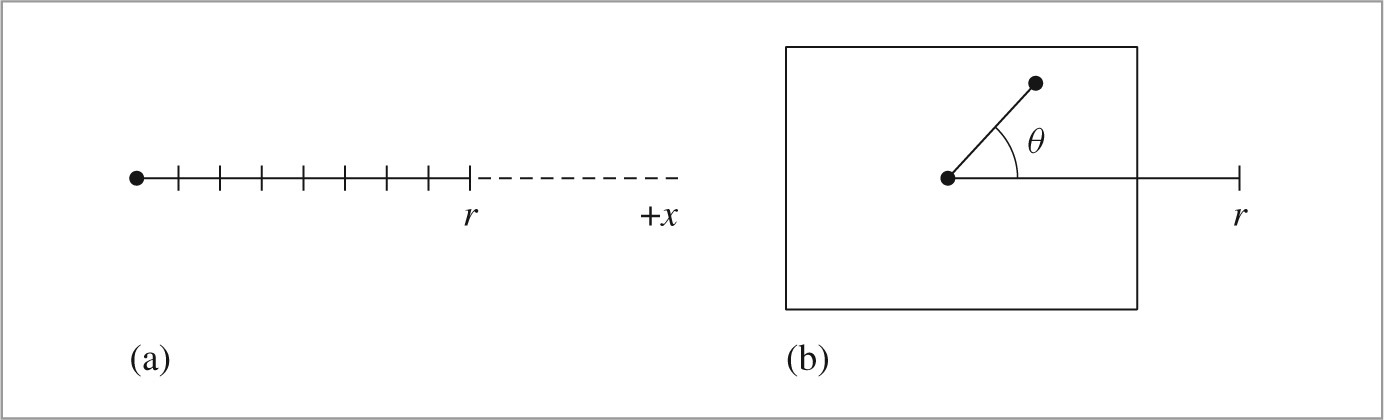
Three more coordinate systems (summarized in Figure 6.1) are useful for defining and discussing projective cameras:
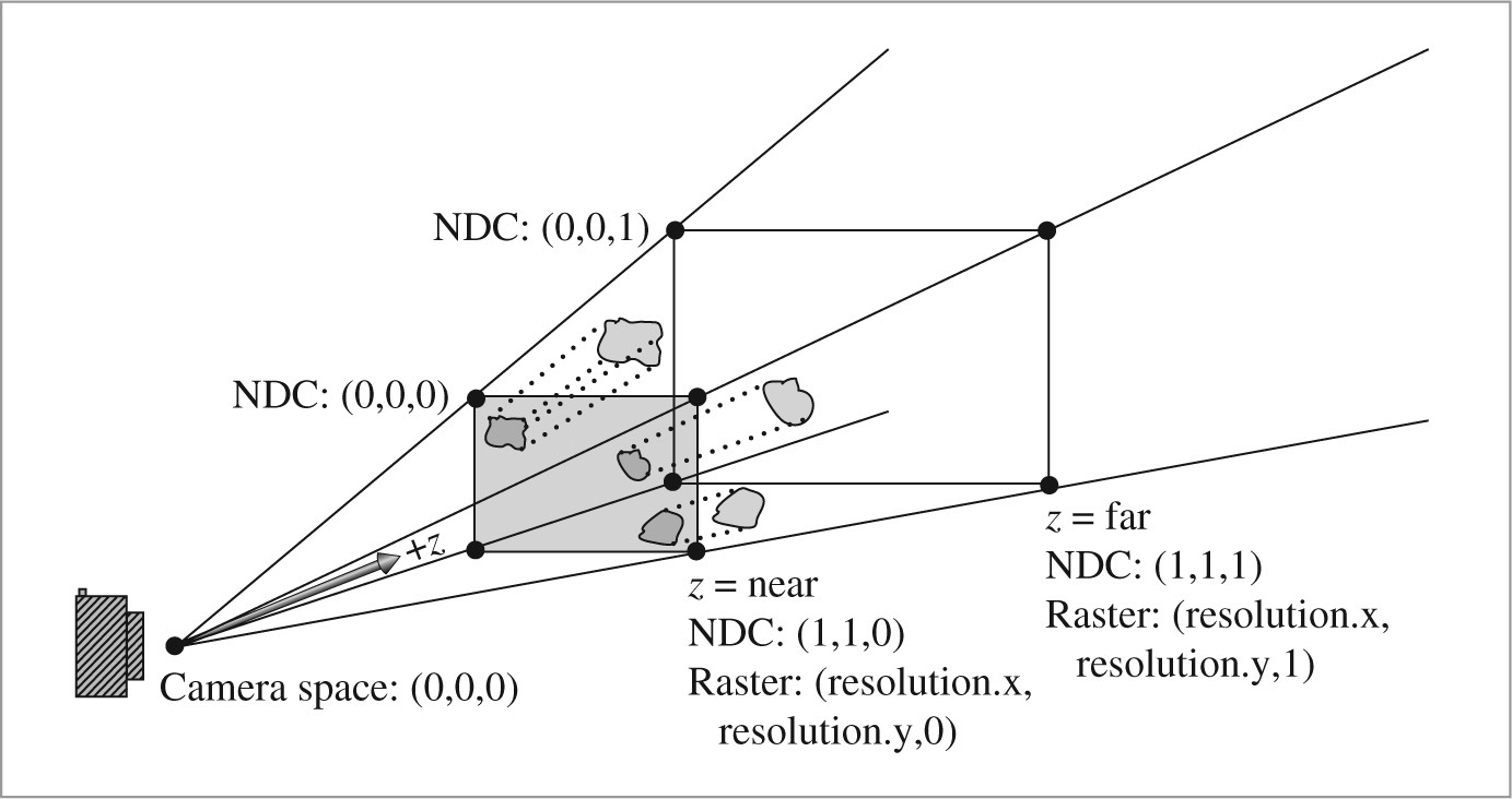
• Screen space: Screen space is defined on the film plane. The camera projects objects in camera space onto the film plane; the parts inside the screen window are visible in the image that is generated. Depth z values in screen space range from 0 to 1, corresponding to points at the near and far clipping planes, respectively. Note that, although this is called “screen” space, it is still a 3D coordinate system, since z values are meaningful.
• Normalized device coordinate (NDC) space: This is the coordinate system for the actual image being rendered. In x and y, this space ranges from (0, 0) to (1, 1), with (0, 0) being the upper-left corner of the image. Depth values are the same as in screen space, and a linear transformation converts from screen to NDC space.
• Raster space: This is almost the same as NDC space, except the x and y coordinates range from (0, 0) to (resolution.x, resolution.y).
Projective cameras use 4 × 4 matrices to transform among all of these spaces, but cameras with unusual imaging characteristics can’t necessarily represent all of these transformations with matrices.
In addition to the parameters required by the Camera base class, the ProjectiveCamera takes the projective transformation matrix, the screen space extent of the image, and additional parameters related to depth of field. Depth of field, which will be described and implemented at the end of this section, simulates the blurriness of out-of-focus objects that occurs in real lens systems.
〈ProjectiveCamera Public Methods〉 ≡ 358
ProjectiveCamera(const AnimatedTransform &CameraToWorld,
const Transform &CameraToScreen, const Bounds2f &screenWindow,
Float shutterOpen, Float shutterClose, Float lensr, Float focald,
Film *film, const Medium *medium)
: Camera(CameraToWorld, shutterOpen, shutterClose, film, medium),
CameraToScreen(CameraToScreen) {
〈Initialize depth of field parameters 374〉
〈Compute projective camera transformations 360〉
}
ProjectiveCamera implementations pass the projective transformation up to the base class constructor shown here. This transformation gives the camera-to-screen projection; from that, the constructor can easily compute the other transformation that will be needed, to go all the way from raster space to camera space.
〈Compute projective camera transformations〉 ≡ 360
〈Compute projective camera screen transformations 360〉
RasterToCamera = Inverse(CameraToScreen) * RasterToScreen;
〈ProjectiveCamera Protected Data〉 ≡ 358
Transform CameraToScreen, RasterToCamera;
The only nontrivial transformation to compute in the constructor is the screen-to-raster projection. In the following code, note the composition of transformations where (reading from bottom to top), we start with a point in screen space, translate so that the upper-left corner of the screen is at the origin, and then scale by the reciprocal of the screen width and height, giving us a point with x and y coordinates between 0 and 1 (these are NDC coordinates). Finally, we scale by the raster resolution, so that we end up covering the entire raster range from (0, 0) up to the overall raster resolution. An important detail here is that the y coordinate is inverted by this transformation; this is necessary because increasing y values move up the image in screen coordinates but down in raster coordinates.
〈Compute projective camera screen transformations〉 ≡ 360
ScreenToRaster = Scale(film- > fullResolution.x,
film- > fullResolution.y, 1) *
Scale(1 / (screenWindow.pMax.x - screenWindow.pMin.x),
1 / (screenWindow.pMin.y - screenWindow.pMax.y), 1) *
Translate(Vector3f(-screenWindow.pMin.x, -screenWindow.pMax.y, 0));
RasterToScreen = Inverse(ScreenToRaster);
〈ProjectiveCamera Protected Data〉 + ≡ 358
Transform ScreenToRaster, RasterToScreen;
6.2.1 Orthographic camera
〈OrthographicCamera Declarations〉 ≡
class OrthographicCamera : public ProjectiveCamera {
public:
〈OrthographicCamera Public Methods 361〉
private:
〈OrthographicCamera Private Data 363〉
};
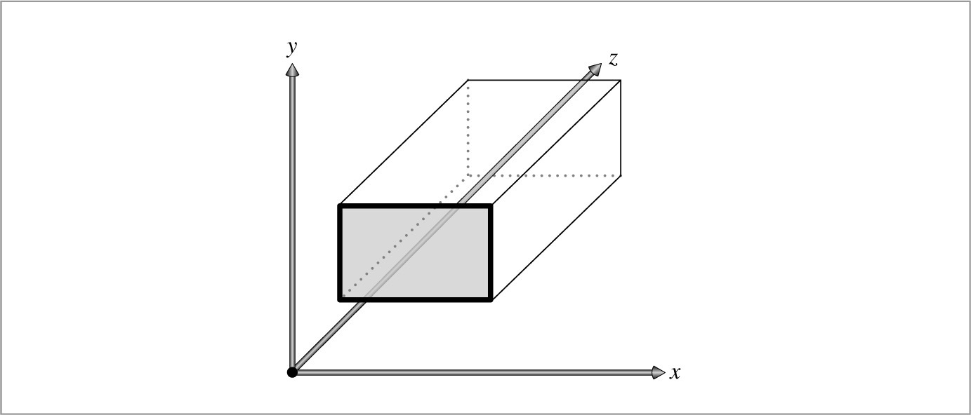
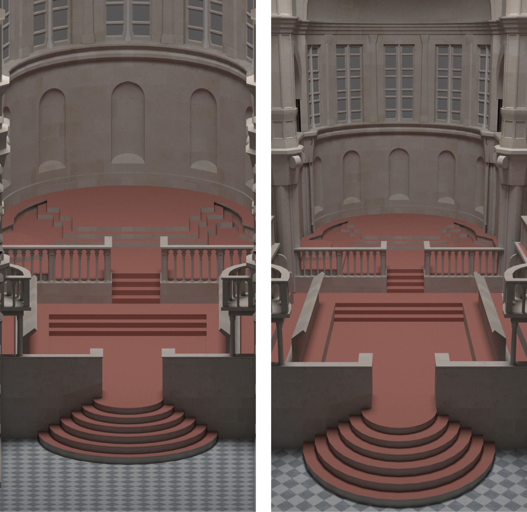
The orthographic camera, defined in the files cameras/orthographic.h and cameras/orthographic.cpp, is based on the orthographic projection transformation. The orthographic transformation takes a rectangular region of the scene and projects it onto the front face of the box that defines the region. It doesn’t give the effect of foreshortening—objects becoming smaller on the image plane as they get farther away—but it does leave parallel lines parallel, and it preserves relative distance between objects. Figure 6.2 shows how this rectangular volume defines the visible region of the scene. Figure 6.3 compares the result of using the orthographic projection for rendering to the perspective projection defined in the next section.
The orthographic camera constructor generates the orthographic transformation matrix with the Orthographic() function, which will be defined shortly.
〈OrthographicCamera Public Methods〉 ≡ 361
OrthographicCamera(const AnimatedTransform &CameraToWorld,
const Bounds2f &screenWindow, Float shutterOpen,
Float shutterClose, Float lensRadius, Float focalDistance,
Film *film, const Medium *medium)
: ProjectiveCamera(CameraToWorld, Orthographic(0, 1),
screenWindow, shutterOpen, shutterClose,
lensRadius, focalDistance, film, medium) {
〈Compute differential changes in origin for orthographic camera rays 363〉
}
The orthographic viewing transformation leaves x and y coordinates unchanged but maps z values at the near plane to 0 and z values at the far plane to 1. To do this, the scene is first translated along the z axis so that the near plane is aligned with z = 0. Then, the scene is scaled in z so that the far plane maps to z = 1. The composition of these two transformations gives the overall transformation. (For a ray tracer like pbrt, we’d like the near plane to be at 0 so that rays start at the plane that goes through the camera’s position; the far plane offset doesn’t particularly matter.)
〈Transform Method Definitions〉 + ≡
Transform Orthographic(Float zNear, Float zFar) {
return Scale(1, 1, 1 / (zFar - zNear)) *
Translate(Vector3f(0, 0, -zNear));
}
Thanks to the simplicity of the orthographic projection, it’s easy to directly compute the differential rays in the x and y directions in the GenerateRayDifferential() method. The directions of the differential rays will be the same as the main ray (as they are for all rays generated by an orthographic camera), and the difference in origins will be the same for all rays. Therefore, the constructor here precomputes how much the ray origins shift in camera space coordinates due to a single pixel shift in the x and y directions on the film plane.
〈Compute differential changes in origin for orthographic camera rays〉 ≡ 361
dxCamera = RasterToCamera(Vector3f(1, 0, 0));
dyCamera = RasterToCamera(Vector3f(0, 1, 0));
〈OrthographicCamera Private Data〉 ≡ 361
Vector3f dxCamera, dyCamera;
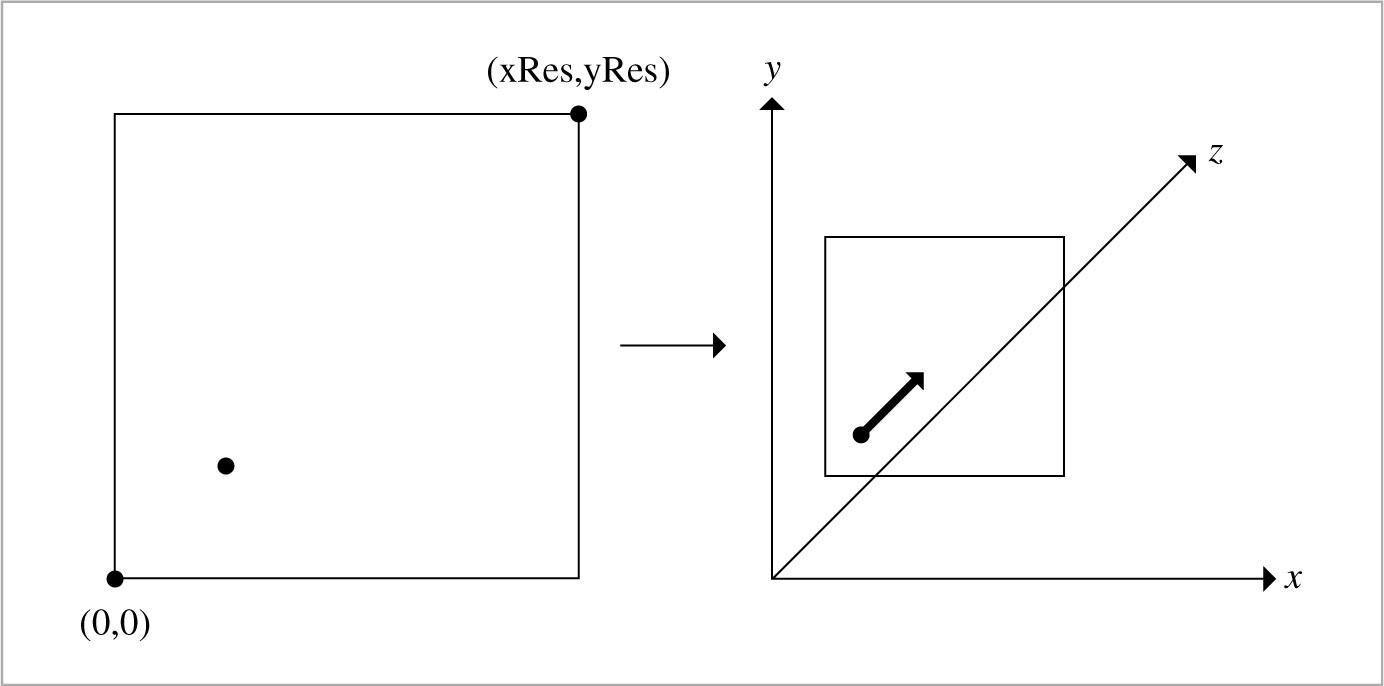
We can now go through the code to take a sample point in raster space and turn it into a camera ray. The process is summarized in Figure 6.4. First, the raster space sample position is transformed into a point in camera space, giving a point located on the near plane, which is the origin of the camera ray. Because the camera space viewing direction points down the z axis, the camera space ray direction is (0, 0, 1).
If depth of field has been enabled for this scene, the ray’s origin and direction are modified so that depth of field is simulated. Depth of field will be explained later in this section. The ray’s time value is set by linearly interpolating between the shutter open and shutter close times by the CameraSample::time offset (which is in the range [0, 1)). Finally, the ray is transformed into world space before being returned.
〈OrthographicCamera Definitions〉 ≡
Float OrthographicCamera::GenerateRay(const CameraSample &sample,
Ray *ray) const {
〈Compute raster and camera sample positions 364〉
*ray = Ray(pCamera, Vector3f(0, 0, 1));
〈Modify ray for depth of field 374〉
ray- > time = Lerp(sample.time, shutterOpen, shutterClose);
ray- > medium = medium;
*ray = CameraToWorld(*ray);
return 1;
}
Once all of the transformation matrices have been set up, it’s easy to transform the raster space sample point to camera space.
〈Compute raster and camera sample positions〉 ≡ 364, 367
Point3f pFilm = Point3f(sample.pFilm.x, sample.pFilm.y, 0);
Point3f pCamera = RasterToCamera(pFilm);
The implementation of GenerateRayDifferential() performs the same computation to generate the main camera ray. The differential ray origins are found using the offsets computed in the OrthographicCamera constructor, and then the full ray differential is transformed to world space.
〈OrthographicCamera Definitions〉 + ≡
Float OrthographicCamera::GenerateRayDifferential(
const CameraSample &sample, RayDifferential *ray) const {
〈Compute main orthographic viewing ray〉
〈Compute ray differentials for OrthographicCamera 364〉
ray- > time = Lerp(sample.time, shutterOpen, shutterClose);
ray- > hasDifferentials = true;
ray- > medium = medium;
*ray = CameraToWorld(*ray);
return 1;
}
〈Compute ray differentials for OrthographicCamera〉 ≡ 364
if (lensRadius > 0) {
〈Compute OrthographicCamera ray differentials accounting for lens〉
} else {
ray- > rxOrigin = ray- > o + dxCamera;
ray- > ryOrigin = ray- > o + dyCamera;
ray- > rxDirection = ray- > ryDirection = ray- > d;
}
6.2.2 Perspective camera
The perspective projection is similar to the orthographic projection in that it projects a volume of space onto a 2D film plane. However, it includes the effect of foreshortening: objects that are far away are projected to be smaller than objects of the same size that are closer. Unlike the orthographic projection, the perspective projection doesn’t preserve distances or angles, and parallel lines no longer remain parallel. The perspective projection is a reasonably close match to how an eye or camera lens generates images of the 3D world. The perspective camera is implemented in the files cameras/perspective.h and cameras/perspective.cpp.
〈PerspectiveCamera Declarations〉 ≡
class PerspectiveCamera : public ProjectiveCamera {
public:
〈PerspectiveCamera Public Methods 367〉
private:
〈PerspectiveCamera Private Data 367〉
};
〈PerspectiveCamera Method Definitions〉 ≡
PerspectiveCamera::PerspectiveCamera(
const AnimatedTransform &CameraToWorld,
const Bounds2f &screenWindow, Float shutterOpen,
Float shutterClose, Float lensRadius, Float focalDistance,
Float fov, Film *film, const Medium *medium)
: ProjectiveCamera(CameraToWorld, Perspective(fov, 1e-2f, 1000.f),
screenWindow, shutterOpen, shutterClose,
lensRadius, focalDistance, film, medium) {
〈Compute differential changes in origin for perspective camera rays 367〉
〈Compute image plane bounds at z = 1 for PerspectiveCamera 951〉
}
The perspective projection describes perspective viewing of the scene. Points in the scene are projected onto a viewing plane perpendicular to the z axis. The Perspective() function computes this transformation; it takes a field-of-view angle in fov and the distances to a near z plane and a far z plane. After the perspective projection, points at the near z plane are mapped to have z = 0, and points at the far plane have z = 1 (Figure 6.5). For rendering systems based on rasterization, it’s important to set the positions of these planes carefully; they determine the z range of the scene that is rendered, but setting them with too many orders of magnitude variation between their values can lead to numerical precision errors. For a ray tracers like pbrt, they can be set arbitrarily as they are here.
〈Transform Method Definitions〉 + ≡
Transform Perspective(Float fov, Float n, Float f) {
〈Perform projective divide for perspective projection 366〉
〈Scale canonical perspective view to specified field of view 367〉
}
The transformation is most easily understood in two steps:
1. Points p in camera space are projected onto the viewing plane. A bit of algebra shows that the projected x′ and y′ coordinates on the viewing plane can be computed by dividing x and y by the point’s z coordinate value. The projected z depth is remapped so that z values at the near plane are 0 and z values at the far plane are 1. The computation we’d like to do is
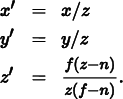
All of this computation can be encoded in a 4 × 4 matrix using homogeneous coordinates:
〈Perform projective divide for perspective projection〉 ≡ 365
Matrix4x4 persp(1, 0, 0, 0,
0, 1, 0, 0,
0, 0, f / (f - n), -f*n / (f - n),
0, 0, 1, 0);
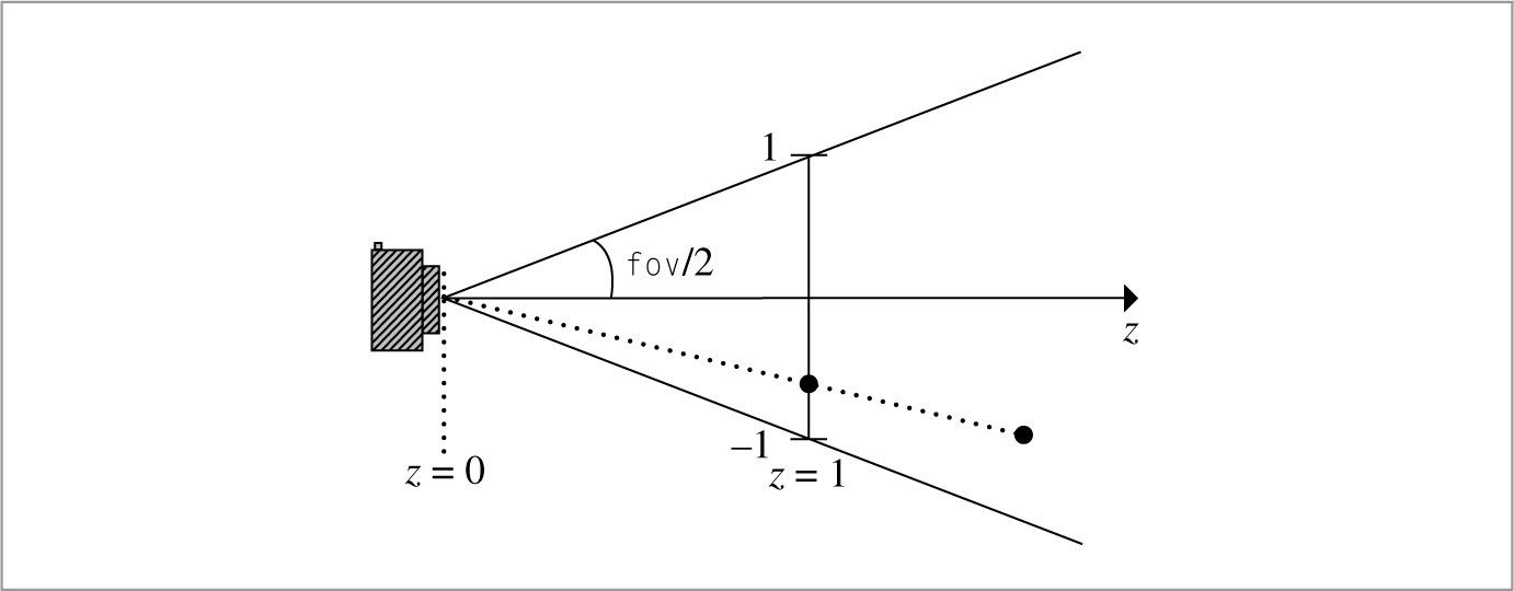
2. The angular field of view (fov) specified by the user is accounted for by scaling the (x, y) values on the projection plane so that points inside the field of view project to coordinates between [− 1, 1] on the view plane. For square images, both x and y lie between [− 1, 1] in screen space. Otherwise, the direction in which the image is narrower maps to [− 1, 1], and the wider direction maps to a proportionally larger range of screen space values. Recall that the tangent is equal to the ratio of the opposite side of a right triangle to the adjacent side. Here the adjacent side has length 1, so the opposite side has the length tan(fov/2). Scaling by the reciprocal of this length maps the field of view to range from [− 1, 1].
〈Scale canonical perspective view to specified field of view〉 ≡ 365
Float invTanAng = 1 / std::tan(Radians(fov) / 2);
return Scale(invTanAng, invTanAng, 1) * Transform(persp);
Similar to the OrthographicCamera, information about how the camera rays generated by the PerspectiveCamera change as we shift pixels on the film plane can be precomputed in the constructor. Here, we compute the change in position on the near perspective plane in camera space with respect to shifts in pixel location.
〈Compute differential changes in origin for perspective camera rays〉 ≡ 365
dxCamera = (RasterToCamera(Point3f(1, 0, 0)) -
RasterToCamera(Point3f(0, 0, 0)));
dyCamera = (RasterToCamera(Point3f(0, 1, 0)) -
RasterToCamera(Point3f(0, 0, 0)));
〈PerspectiveCamera Private Data〉 ≡ 365
Vector3f dxCamera, dyCamera;
With the perspective projection, all rays originate from the origin, (0, 0, 0), in camera space. A ray’s direction is given by the vector from the origin to the point on the near plane, pCamera, that corresponds to the provided CameraSample’s pFilm location. In other words, the ray’s vector direction is component-wise equal to this point’s position, so rather than doing a useless subtraction to compute the direction, we just initialize the direction directly from the point pCamera.
〈PerspectiveCamera Method Definitions〉 + ≡
Float PerspectiveCamera::GenerateRay(const CameraSample &sample,
Ray *ray) const {
〈Compute raster and camera sample positions 364〉
*ray = Ray(Point3f(0, 0, 0), Normalize(Vector3f(pCamera)));
〈Modify ray for depth of field 374〉
ray- > time = Lerp(sample.time, shutterOpen, shutterClose);
ray- > medium = medium;
*ray = CameraToWorld(*ray);
return 1;
}
The GenerateRayDifferential() method follows the implementation of GenerateRay(), except for an additional fragment that computes the differential rays.
〈PerspectiveCamera Public Methods〉 ≡ 365
Float GenerateRayDifferential(const CameraSample &sample,
RayDifferential *ray) const;
〈Compute offset rays for PerspectiveCamera ray differentials〉 ≡
if (lensRadius > 0) {
〈Compute PerspectiveCamera ray differentials accounting for lens〉
} else {
ray- > rxOrigin = ray- > ryOrigin = ray- > o;
ray- > rxDirection = Normalize(Vector3f(pCamera) + dxCamera);
ray- > ryDirection = Normalize(Vector3f(pCamera) + dyCamera);
}
6.2.3 The thin lens model and depth of field
An ideal pinhole camera that only allows rays passing through a single point to reach the film isn’t physically realizable; while it’s possible to make cameras with extremely small apertures that approach this behavior, small apertures allow relatively little light to reach the film sensor. With a small aperture, long exposure times are required to capture enough photons to accurately capture the image, which in turn can lead to blur from objects in the scene moving while the camera shutter is open.
Real cameras have lens systems that focus light through a finite-sized aperture onto the film plane. Camera designers (and photographers using cameras with adjustable apertures) face a trade-off: the larger the aperture, the more light reaches the film and the shorter the exposures that are needed. However, lenses can only focus on a single plane (the focal plane), and the farther objects in the scene are from this plane, the blurrier they are. The larger the aperture, the more pronounced this effect is: objects at depths different from the one the lens system has in focus become increasingly blurry.
The camera model in Section 6.4 implements a fairly accurate simulation of lens systems in realistic cameras. For the simple camera models introduced so far, we can apply a classic approximation from optics, the thin lens approximation, to model the effect of finite apertures with traditional computer graphics projection models. The thin lens approximation models an optical system as a single lens with spherical profiles, where the thickness of the lens is small relative to the radius of curvature of the lens. (The more general thick lens approximation, which doesn’t assume that the lens’s thickness is negligible, is introduced in Section 6.4.3.)
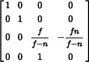
Under the thin lens approximation, parallel incident rays passing through the lens focus at a point called behind the lens called the focal point. The distance the focal point is behind the lens, f, is the lens’s focal length. If the film plane is placed at a distance equal to the focal length behind the lens, then objects infinitely far away will be in focus, as they image to a single point on the film.
Figure 6.6 illustrates the basic setting. Here we’ve followed the typical lens coordinate system convention of placing the lens perpendicular to the z axis, with the lens at z = 0 and the scene along − z. (Note that this is a different coordinate system from the one we used for camera space, where the viewing direction is + z.) Distances on the scene side of the lens are denoted with unprimed variables z, and distances on the film side of the lens (positive z) are primed, z′.
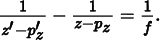
For points in the scene at a depth z from a thin lens with focal length f, the Gaussian lens equation relates the distances from the object to the lens and from lens to the image of the point:
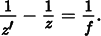
Note that for z = −∞, we have z′ = f, as expected.
We can use the Gaussian lens equation to solve for the distance between the lens and the film that sets the plane of focus at some z, the focal distance (Figure 6.7):

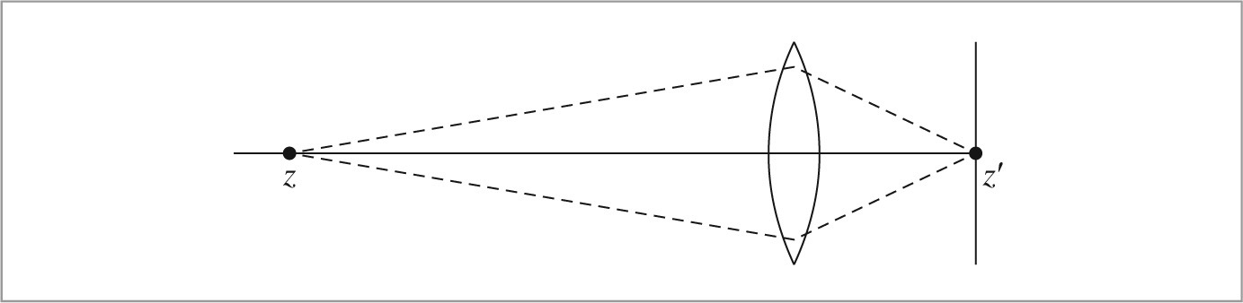
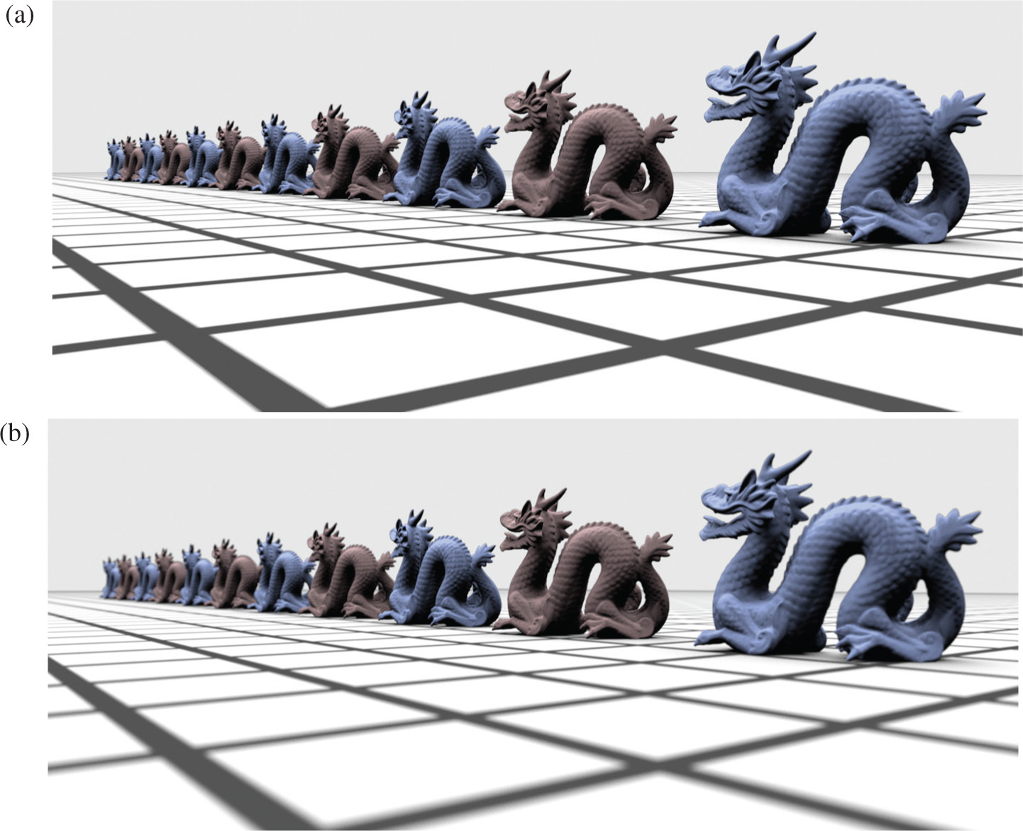
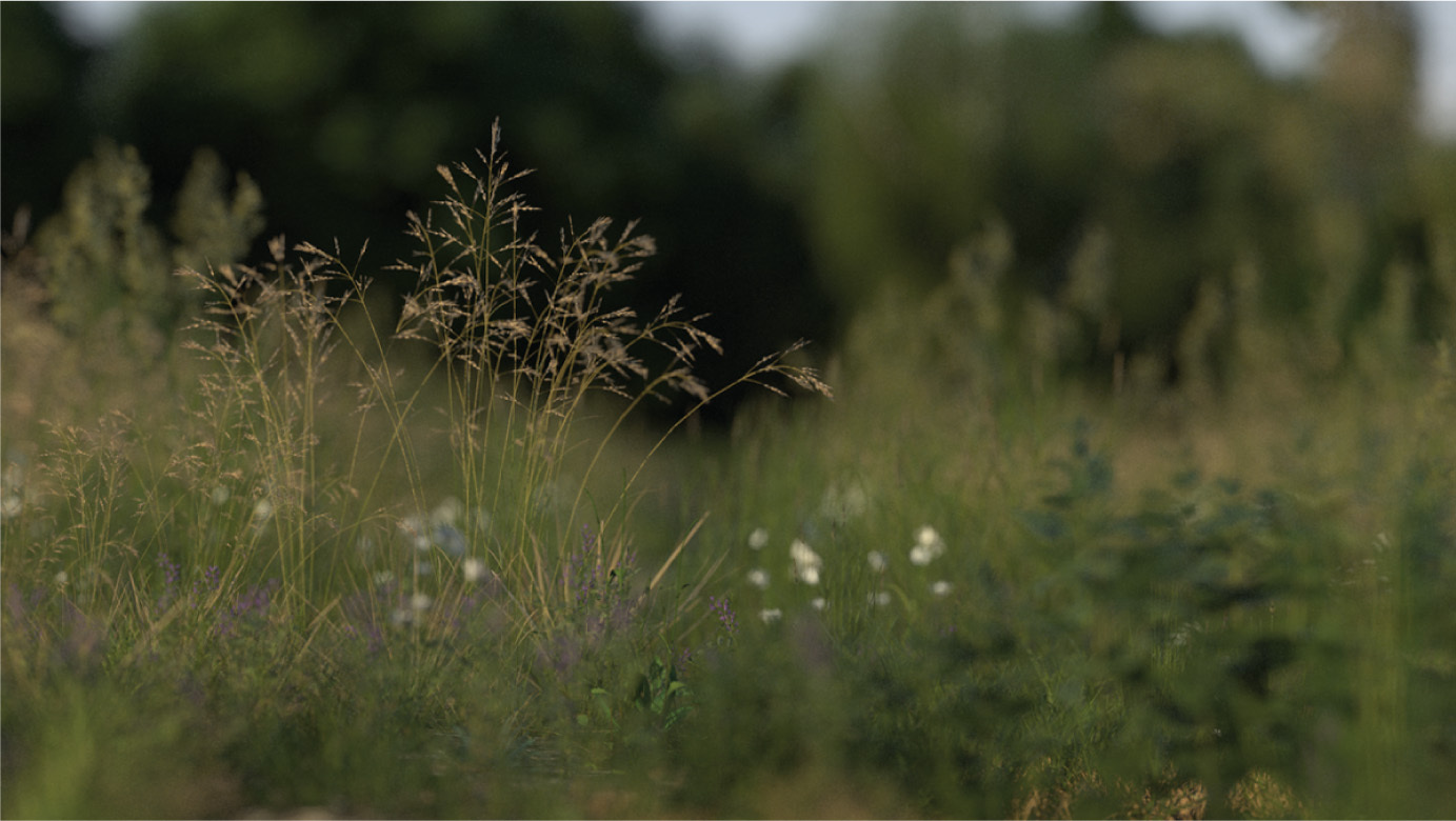
A point that doesn’t lie on the plane of focus is imaged to a disk on the film plane, rather than to a single point. This boundary of this disk is called the circle of confusion. The size of the circle of confusion is affected by the diameter of the aperture that light rays pass through, the focal distance, and the distance between the object and the lens. Figures 6.8 and 6.9 show this effect, depth of field, in a scene with a series of copies of the dragon model. Figure 6.8(a) is rendered with an infinitesimal aperture and thus without any depth of field effects. Figures 6.8(b) and 6.9 show the increase in blurriness as the size of the lens aperture is increased. Note that the second dragon from the right remains in focus throughout all of the images, as the plane of focus has been placed at its depth. Figure 6.10 shows depth of field used to render the landscape scene. Note how the effect draws the viewer’s eye to the in-focus grass in the center of the image.
In practice, objects do not have to be exactly on the plane of focus to appear in sharp focus; as long as the circle of confusion is roughly smaller than a pixel on the film sensor, objects appear to be in focus. The range of distances from the lens at which objects appear in focus is called the lens’s depth of field.
The Gaussian lens equation also lets us compute the size of the circle of confusion; given a lens with focal length f that is focused at a distance zf, the film plane is at zf′. Given another point at depth z, the Gaussian lens equation gives the distance z′ that the lens focuses the point to. This point is either in front of or behind the film plane; Figure 6.11(a) shows the case where it is behind.
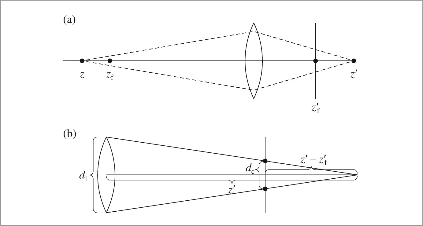
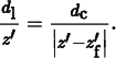
The diameter of the circle of confusion is given by the intersection of the cone between z′ and the lens with the film plane. If we know the diameter of the lens dl, then we can use similar triangles to solve for the diameter of the circle of confusion dc (Figure 6.11(b)):
Solving for dc, we have
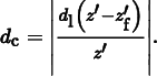
Applying the Gaussian lens equation to express the result in terms of scene depths, we can find that
Note that the diameter of the circle of confusion is proportional to the diameter of the lens. The lens diameter is often expressed as the lens’s f-number n, which expresses diameter as a fraction of focal length, dl = f/n.
Figure 6.12 shows a graph of this function for a 50-mm focal length lens with a 25-mm aperture, focused at zf = 1 m. Note that the blur is asymmetric with depth around the focal plane and grows much more quickly for objects in front of the plane of focus than for objects behind it.
Modeling a thin lens in a ray tracer is remarkably straightforward: all that is necessary is to choose a point on the lens and find the appropriate ray that starts on the lens at that point such that objects in the plane of focus are in focus on the film (Figure 6.13).
Therefore, projective cameras take two extra parameters for depth of field: one sets the size of the lens aperture, and the other sets the focal distance.
〈ProjectiveCamera Protected Data〉 + ≡ 358
Float lensRadius, focalDistance;
〈Initialize depth of field parameters〉 ≡ 360
lensRadius = lensr;
focalDistance = focald;
It is generally necessary to trace many rays for each image pixel in order to adequately sample the lens for smooth depth of field. Figure 6.14 shows the landscape scene from Figure 6.10 with only four samples per pixel (Figure 6.10 had 128 samples per pixel).
〈Modify ray for depth of field〉 ≡ 364, 367
if (lensRadius > 0) {
〈Sample point on lens 374〉
〈Compute point on plane of focus 375〉
〈Update ray for effect of lens 375〉
}
The ConcentricSampleDisk() function, defined in Chapter 13, takes a (u, v) sample position in [0, 1)2 and maps it to a 2D unit disk centered at the origin (0, 0). To turn this into a point on the lens, these coordinates are scaled by the lens radius. The CameraSample class provides the (u, v) lens-sampling parameters in the pLens member variable.
〈Sample point on lens〉 ≡ 374
Point2f pLens = lensRadius * ConcentricSampleDisk(sample.pLens);
The ray’s origin is this point on the lens. Now it is necessary to determine the proper direction for the new ray. We know that all rays from the given image sample through the lens must converge at the same point on the plane of focus. Furthermore, we know that rays pass through the center of the lens without a change in direction, so finding the appropriate point of convergence is a matter of intersecting the unperturbed ray from the pinhole model with the plane of focus and then setting the new ray’s direction to be the vector from the point on the lens to the intersection point.
For this simple model, the plane of focus is perpendicular to the z axis and the ray starts at the origin, so intersecting the ray through the lens center with the plane of focus is straightforward. The t value of the intersection is given by
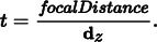
〈Compute point on plane of focus〉 ≡ 374
Float ft = focalDistance / ray- > d.z;
Point3f pFocus = (*ray)(ft);
Now the ray can be initialized. The origin is set to the sampled point on the lens, and the direction is set so that the ray passes through the point on the plane of focus, pFocus.
〈Update ray for effect of lens〉 ≡ 374
ray- > o = Point3f(pLens.x, pLens.y, 0);
ray- > d = Normalize(pFocus - ray- > o);
To compute ray differentials with the thin lens, the approach used in the fragment 〈Update ray for effect of lens〉 is applied to rays offset one pixel in the x and y directions on the film plane. The fragments that implement this, 〈Compute OrthographicCamera ray differentials accounting for lens〉 and 〈Compute PerspectiveCamera ray differentials accounting for lens〉, aren’t included here.
6.3 Environment camera
One advantage of ray tracing compared to scan line or rasterization-based rendering methods is that it’s easy to employ unusual image projections. We have great freedom in how the image sample positions are mapped into ray directions, since the rendering algorithm doesn’t depend on properties such as straight lines in the scene always projecting to straight lines in the image.
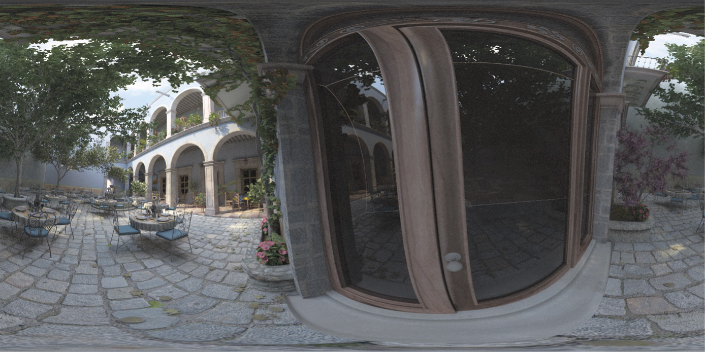
In this section, we will describe a camera model that traces rays in all directions around a point in the scene, giving a 2D view of everything that is visible from that point. Consider a sphere around the camera position in the scene; choosing points on that sphere gives directions to trace rays in. If we parameterize the sphere with spherical coordinates, each point on the sphere is associated with a (θ, ϕ) pair, where θ ∈ [0, π] and ϕ ∈ [0, 2π]. (See Section 5.5.2 for more details on spherical coordinates.) This type of image is particularly useful because it represents all of the incident light at a point on the scene. (One important use of this image representation is environment lighting—a rendering technique that uses image-based representations of light in a scene.) Figure 6.15 shows this camera in action with the San Miguel model. θ values range from 0 at the top of the image to π at the bottom of the image, and ϕ values range from 0 to 2π, moving from left to right across the image.1
〈EnvironmentCamera Declarations〉 ≡
class EnvironmentCamera : public Camera {
public:
〈EnvironmentCamera Public Methods 376〉
};
The EnvironmentCamera derives directly from the Camera class, not the ProjectiveCamera class. This is because the environmental projection is nonlinear and cannot be captured by a single 4 × 4 matrix. This camera is defined in the files cameras/environment.h and cameras/environment.cpp.
〈EnvironmentCamera Public Methods〉 ≡ 376
EnvironmentCamera(const AnimatedTransform &CameraToWorld,
Float shutterOpen, Float shutterClose, Film *film,
const Medium *medium)
: Camera(CameraToWorld, shutterOpen, shutterClose, film, medium) {
}
〈EnvironmentCamera Method Definitions〉 ≡
Float EnvironmentCamera::GenerateRay(const CameraSample &sample,
Ray *ray) const {
〈Compute environment camera ray direction 377〉
*ray = Ray(Point3f(0, 0, 0), dir, Infinity,
Lerp(sample.time, shutterOpen, shutterClose));
ray- > medium = medium;
*ray = CameraToWorld(*ray); return 1;
To compute the (θ, ϕ) coordinates for this ray, NDC coordinates are computed from the raster image sample position and then scaled to cover the (θ, ϕ) range. Next, the spherical coordinate formula is used to compute the ray direction, and finally the direction is converted to world space. (Note that because the y direction is “up” in camera space, here the y and z coordinates in the spherical coordinate formula are exchanged in comparison to usage elsewhere in the system.)
〈Compute environment camera ray direction〉 ≡ 377
Float theta = Pi * sample.pFilm.y / film- > fullResolution.y;
Float phi = 2 * Pi * sample.pFilm.x / film- > fullResolution.x;
Vector3f dir(std::sin(theta) * std::cos(phi), std::cos(theta),
std::sin(theta) * std::sin(phi));
*6.4 Realistic cameras
The thin lens model makes it possible to render images with blur due to depth of field, but it is a fairly rough approximation of actual camera lens systems, which are comprised of a series of multiple lens elements, each of which modifies the distribution of radiance passing through it. (Figure 6.16 shows a cross section of a 22-mm focal length wide-angle lens with eight elements.) Even basic cell phone cameras tend to have on the order of five individual lens elements, while DSLR lenses may have ten or more. In general, more complex lens systems with larger numbers of lens elements can create higher quality images than simpler lens systems.

This section discusses the implementation of RealisticCamera, which simulates the focusing of light through lens systems like the one in Figure 6.16 to render images like Figure 6.17. Its implementation is based on ray tracing, where the camera follows ray paths through the lens elements, accounting for refraction at the interfaces between media (air, different types of glass) with different indices of refraction, until the ray path either exits the optical system or until it is absorbed by the aperture stop or lens housing. Rays leaving the front lens element represent samples of the camera’s response profile and can be used with integrators that estimate the incident radiance along arbitrary rays, such as the SamplerIntegrator. The RealisticCamera implementation is in the files cameras/realistic.h and cameras/realistic.cpp.
〈RealisticCamera Declarations〉 ≡
class RealisticCamera : public Camera
{ public:
〈RealisticCamera Public Methods〉
private:
〈RealisticCamera Private Declarations 381〉
〈RealisticCamera Private Data 379〉
〈RealisticCamera Private Methods 381〉
};
In addition to the usual transformation to place the camera in the scene, the Film, and the shutter open and close times, the RealisticCamera constructor takes a filename for a lens system description file, the distance to the desired plane of focus, and a diameter for the aperture stop. The effect of the simpleWeighting parameter is described later, in Section 13.6.6, after preliminaries related to Monte Carlo integration in Chapter 13 and the radiometry of image formation in Section 6.4.7.
〈RealisticCamera Method Definitions〉 ≡
RealisticCamera::RealisticCamera(const AnimatedTransform &CameraToWorld,
Float shutterOpen, Float shutterClose, Float apertureDiameter,
Float focusDistance, bool simpleWeighting, const char *lensFile,
Film *film, const Medium *medium)
: Camera(CameraToWorld, shutterOpen, shutterClose, film, medium),
simpleWeighting(simpleWeighting) {
〈Load element data from lens description file〉
〈Compute lens–film distance for given focus distance 389〉
〈Compute exit pupil bounds at sampled points on the film 390〉
}
〈RealisticCamera Private Data〉 ≡ 378
const bool simpleWeighting;
After loading the lens description file from disk, the constructor adjusts the spacing between the lenses and the film so that the plane of focus is at the desired depth, focusDistance, and then precomputes some information about which areas of the lens element closest to the film carry light from the scene to the film, as seen from various points on the film plane. After background material has been introduced, the fragments 〈Compute lens–film distance for given focus distance〉 and 〈Compute exit pupil bounds at sampled points on the film〉 will be defined in Sections 6.4.4 and 6.4.5, respectively.
6.4.1 Lens system representation
A lens system is made from a series of lens elements, where each element is generally some form of glass. A lens system designer’s challenge is to design a series of elements that form high-quality images on a film or sensor subject to limitations of space (e.g., the thickness of mobile phone cameras is very limited in order to keep phones thin), cost, and ease of manufacture.
It’s easiest to manufacture lenses with cross sections that are spherical, and lens systems are generally symmetric around the optical axis, which is conventionally denoted by z. We will assume both of these properties in the remainder of this section. As in Section 6.2.3, lens systems are defined using a coordinate system where the film is aligned with the z = 0 plane and lenses are to the left of the film, along the − z axis.
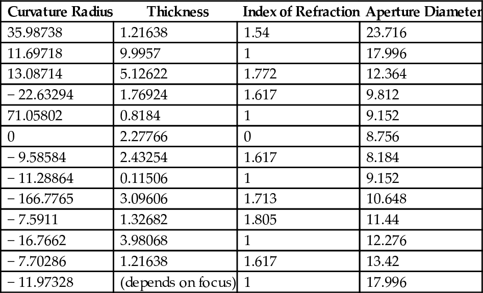
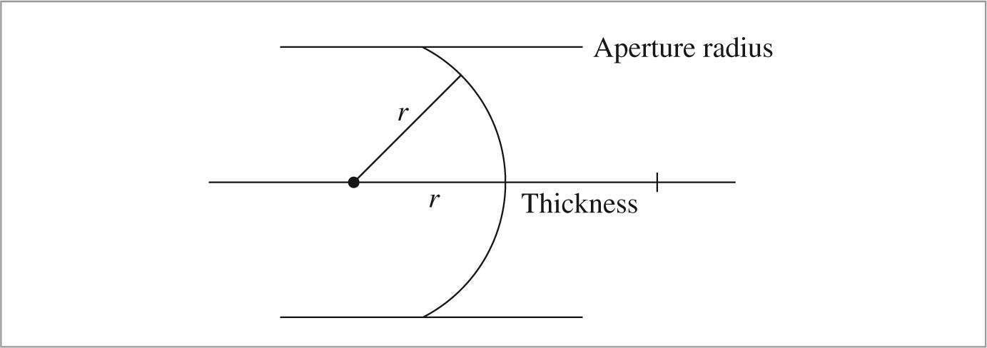
Lens systems are commonly represented in terms of the series of interfaces between the individual lens elements (or air) rather than having an explicit representation of each element. Table 6.1 shows the quantities that define each interface. The last entry in the table defines the rightmost interface, which is shown in Figure 6.18: it’s a section of a sphere with radius equal to the curvature radius. The thickness of an element is the distance along z to the next element to the right (or to the film plane), and the index of refraction is for the medium to the right of the interface. The element’s extent above and below the z axis is set by the aperture diameter.
Table 6.1
Tabular description of the lens system in Figure 6.16. Each line describes the interface between two lens elements, the interface between an element and air, or the aperture stop. The first line describes the leftmost interface. The element with radius 0 corresponds to the aperture stop. Distances are measured in mm.
| Curvature Radius | Thickness | Index of Refraction | Aperture Diameter |
| 35.98738 | 1.21638 | 1.54 | 23.716 |
| 11.69718 | 9.9957 | 1 | 17.996 |
| 13.08714 | 5.12622 | 1.772 | 12.364 |
| − 22.63294 | 1.76924 | 1.617 | 9.812 |
| 71.05802 | 0.8184 | 1 | 9.152 |
| 0 | 2.27766 | 0 | 8.756 |
| − 9.58584 | 2.43254 | 1.617 | 8.184 |
| − 11.28864 | 0.11506 | 1 | 9.152 |
| − 166.7765 | 3.09606 | 1.713 | 10.648 |
| − 7.5911 | 1.32682 | 1.805 | 11.44 |
| − 16.7662 | 3.98068 | 1 | 12.276 |
| − 7.70286 | 1.21638 | 1.617 | 13.42 |
| − 11.97328 | (depends on focus) | 1 | 17.996 |
The LensElementInterface structure represents a single lens element interface.
〈RealisticCamera Private Declarations〉 ≡ 378
struct LensElementInterface {
Float curvatureRadius;
Float thickness;
Float eta;
Float apertureRadius;
};
The fragment 〈Load element data from lens description file〉, not included here, reads the lens elements and initializes the RealisticCamera::elementInterfaces array. See comments in the source code for details of the file format, which parallels the structure of Table 6.1, and see the directory scenes/lenses in the pbrt distribution for a number of example lens descriptions.
Two adjustments are made to the values read from the file: first, lens systems are traditionally described in units of millimeters, but pbrt assumes a scene measured in meters. Therefore, the fields other than the index of refraction are scaled by 1/1000. Second, the element’s diameter is divided by two; the radius is a more convenient quantity to have at hand in the code to follow.
〈RealisticCamera Private Data〉 + ≡ 378
std::vector < LensElementInterface > elementInterfaces;
Once the element interface descriptions have been loaded, it’s useful to have a few values related to the lens system easily at hand. LensRearZ() and LensFrontZ() return the z depths of the rear and front elements of the lens system, respectively. Note that the returned z depths are in camera space, not lens space, and thus have positive values.
〈RealisticCamera Private Methods〉 ≡ 378
Float LensRearZ() const {
return elementInterfaces.back().thickness;
}
Finding the front element’s z position requires summing all of the element thicknesses (see Figure 6.19). This value isn’t needed in any code that is in a performance-sensitive part of the system, so recomputing it when needed is fine. If performance of this method was a concern, it would be better to cache this value in the RealisticCamera.

〈RealisticCamera Private Methods〉 + ≡ 378
Float LensFrontZ() const {
Float zSum = 0;
for (const LensElementInterface &element : elementInterfaces)
zSum + = element.thickness;
return zSum;
}
RearElementRadius() returns the aperture radius of the rear element in meters.
〈RealisticCamera Private Methods〉 + ≡ 378
Float RearElementRadius() const {
return elementInterfaces.back().apertureRadius;
}
6.4.2 Tracing rays through lenses
Given a ray starting from the film side of the lens system, TraceLensesFromFilm() computes intersections with each element in turn, terminating the ray and returning false if its path is blocked along the way through the lens system. Otherwise it returns true and initializes *rOut with the exiting ray in camera space. During traversal, elementZ tracks the z intercept of the current lens element. Because the ray is starting from the film, the lenses are traversed in reverse order compared to how they are stored in elementInterfaces.
〈RealisticCamera Method Definitions〉 + ≡
bool RealisticCamera::TraceLensesFromFilm(const Ray &rCamera,
Ray *rOut) const {
Float elementZ = 0;
〈Transform rCamera from camera to lens system space 383〉
for (int i = elementInterfaces.size() - 1; i > = 0; --i) {
const LensElementInterface &element = elementInterfaces[i];
〈Update ray from film accounting for interaction with element 383〉
}
〈Transform rLens from lens system space back to camera space 385〉
return true;
}
Because the camera points down the + z axis in pbrt’s camera space but lenses are along − z, the z components of the origin and direction of the ray need to be negated. While this is a simple enough transformation that it could be applied directly, we prefer an explicit Transform to make the intent clear.
〈Transform rCamera from camera to lens system space〉 ≡ 382
static const Transform CameraToLens = Scale(1, 1, -1);
Ray rLens = CameraToLens(rCamera);
Recall from Figure 6.19 how the z intercept of elements is computed: because we are visiting the elements from back-to-front, the element’s thickness must be subtracted from elementZ to compute its z intercept before the element interaction is accounted for.
〈Update ray from film accounting for interaction with element〉 ≡ 382
elementZ - = element.thickness;
〈Compute intersection of ray with lens element 383〉
〈Test intersection point against element aperture 384〉
〈Update ray path for element interface interaction 385〉
Given the element’s z axis intercept, the next step is to compute the parametric t value along the ray where it intersects the element interface (or the plane of the aperture stop). For the aperture stop, a ray–plane test (following Section 3.1.2) is used. For spherical interfaces, IntersectSphericalElement() performs this test and also returns the surface normal if an intersection is found; the normal will be needed for computing the refracted ray direction.
〈Compute intersection of ray with lens element〉 ≡ 383
Float t;
Normal3f n;
bool isStop = (element.curvatureRadius == 0);
if (isStop)
t = (elementZ - rLens.o.z) / rLens.d.z;
else {
Float radius = element.curvatureRadius;
Float zCenter = elementZ + element.curvatureRadius;
if (!IntersectSphericalElement(radius, zCenter, rLens, &t, &n))
return false;
}
The IntersectSphericalElement() method is generally similar to Sphere::Intersect(), though it’s specialized for the fact that the element’s center is along the z axis (and thus, the center’s x and y components are zero). The fragments 〈Compute t0 and t1 for ray–element intersection〉 and 〈Compute surface normal of element at ray intersection point〉 aren’t included in the text here due to their similarity with the Sphere::Intersect() implementation.
〈RealisticCamera Method Definitions〉 + ≡
bool RealisticCamera::IntersectSphericalElement(Float radius,
Float zCenter, const Ray &ray, Float *t, Normal3f *n) {
〈Compute t0 and t1 for ray–element intersection〉
〈Select intersection t based on ray direction and element curvature 384〉
〈Compute surface normal of element at ray intersection point 〉
return true;
}
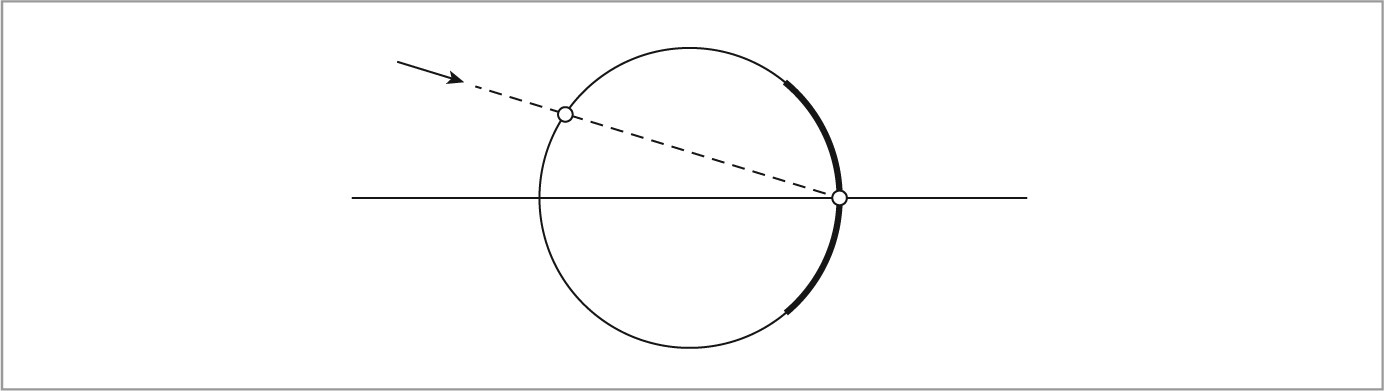
There is, however, a subtlety in choosing which intersection point to return: the closest intersection with t > 0 isn’t necessarily on the element interface; see Figure 6.20.2 For example, for a ray approaching from the scene and intersecting a concave lens (with negative curvature radius), the farther of the two intersections should be returned regardless of whether the closer one has t > 0. Fortunately, simple logic based on the ray direction and the curvature radius indicates which t value to use.
〈Select intersection t based on ray direction and element curvature〉 ≡ 383
bool useCloserT = (ray.d.z > 0) ^ (radius < 0);
*t = useCloserT ? std::min(t0, t1) : std::max(t0, t1);
if (*t < 0)
return false;
Each lens element extends for some radius around the optical axis; if the intersection point with the element is outside this radius, then the ray will actually intersect the lens housing and terminate. In a similar fashion, if a ray intersects the aperture stop, it also terminates. Therefore, here we test the intersection point against the appropriate limit for the current element, either terminating the ray or updating its origin to the current intersection point if it survives.
〈Test intersection point against element aperture〉 ≡ 383
Point3f pHit = rLens(t);
Float r2 = pHit.x * pHit.x + pHit.y * pHit.y;
if (r2 > element.apertureRadius * element.apertureRadius)
return false;
rLens.o = pHit;
If the current element is the aperture, the ray’s path isn’t affected by traveling through the element’s interface. For glass (or, forbid, plastic) lens elements, the ray’s direction changes at the interface as it goes from a medium with one index of refraction to one with another. (The ray may be passing from air to glass, from glass to air, or from glass with one index of refraction to a different type of glass with a different index of refraction.) Section 8.2 discusses how a change in index of refraction at the boundary between two media changes the direction of a ray and the amount of radiance carried by the ray. (In this case, we can ignore the change of radiance, as it cancels out if the ray is in the same medium going into the lens system as it is when it exits—here, both are air.) The Refract() function is defined in Section 8.2.3; note that it expects that the incident direction will point away from the surface, so the ray direction is negated before being passed to it. This function returns false in the presence of total internal reflection, in which case the ray path terminates. Otherwise, the refracted direction is returned in w.
In general, some light passing through an interface like this is transmitted and some is reflected. Here we ignore reflection and assume perfect transmission. Though an approximation, it is a reasonable one: lenses are generally manufactured with coatings designed to reduce the reflection to around 0.25% of the radiance carried by the ray. (However, modeling this small amount of reflection can be important for capturing effects like lens flare.)
〈Update ray path for element interface interaction〉 ≡ 383
if (!isStop) {
Vector3f w;
Float etaI = element.eta;
Float etaT = (i > 0 && elementInterfaces[i - 1].eta ! = 0) ?
elementInterfaces[i - 1].eta : 1;
if (!Refract(Normalize(-rLens.d), n, etaI / etaT, &w))
return false;
rLens.d = w;
}
If the ray has successfully made it out of the front lens element, it just needs to be transformed from lens space to camera space.
〈Transform rLens from lens system space back to camera space〉 ≡ 382
if (rOut ! = nullptr) {
static const Transform LensToCamera = Scale(1, 1, -1);
*rOut = LensToCamera(rLens);
}
The TraceLensesFromScene() method is quite similar to TraceLensesFromFilm() and isn’t included here. The main differences are that it traverses the elements from front-to-back rather than back-to-front. Note that it assumes that the ray passed to it is already in camera space; the caller is responsible for performing the transformation if the ray is starting from world space. The returned ray is in camera space, leaving the rear lens element toward the film.
〈RealisticCamera Private Methods〉 + ≡ 378
bool TraceLensesFromScene(const Ray &rCamera, Ray *rOut) const;
6.4.3 The thick lens approximation
The thin lens approximation used in Section 6.2.3 was based on the simplifying assumption that the lens system had 0 thickness along the optical axis. The thick lens approximation of a lens system is slightly more accurate in that it accounts for the lens system’s z extent. After introducing the basic concepts of the thick lenses here, we’ll use the thick lens approximation to determine how far to place the lens system from the film in order to focus at the desired focal depth in Section 6.4.4.
The thick lens approximation represents a lens system by two pairs of distances along the optical axis—the focal points and the depths of the principal planes; these are two of the cardinal points of a lens system. If rays parallel to the optical axis are traced through an ideal lens system, all of the rays will intersect the optical axis at the same point—this is the focal point. (In practice, real lens systems aren’t perfectly ideal and incident rays at different heights will intersect the optical axis along a small range of z values—this is the spherical aberration.) Given a specific lens system, we can trace rays parallel to the optical axis through it from each side and compute their intersections with the z axis to find the focal points. (See Figure 6.21.)
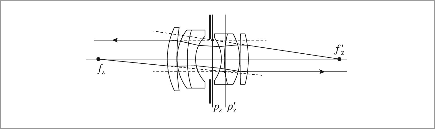
Each principal plane is found by extending the incident ray parallel to the optical axis and the ray leaving the lens until they intersect; the z depth of the intersection gives the depth of the corresponding principal plane. Figure 6.21 shows a lens system with its focal points fz and fz′ and principal planes at z values pz and pz′. (As in Section 6.2.3, primed variables represent points on the film side of the lens system, and unprimed variables represent points in the scene being imaged.)
Given the ray leaving the lens, finding the focal point requires first computing the tf value where the ray’s x and y components are zero. If the entering ray was offset from the optical axis only along x, then we’d like to find tf such that ox + tfdx = 0. Thus,
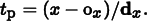
In a similar manner, to find the tp for the principal plane where the ray leaving the lens has the same x height as the original ray, we have ox + tpdx = x, and so
Once these two t values have been computed, the ray equation can be used to find the z coordinates of the corresponding points.
The ComputeCardinalPoints() method computes the z depths of the focal point and the principal plane for the given rays. Note that it assumes that the rays are in camera space but returns z values along the optical axis in lens space.
〈RealisticCamera Method Definitions〉 + ≡
void RealisticCamera::ComputeCardinalPoints(const Ray &rIn,
const Ray &rOut, Float *pz, Float *fz) {
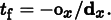
Float tf = -rOut.o.x / rOut.d.x;
*fz = -rOut(tf).z;
Float tp = (rIn.o.x - rOut.o.x) / rOut.d.x;
*pz = -rOut(tp).z;
}
The ComputeThickLensApproximation() method computes both pairs of cardinal points for the lens system.
〈RealisticCamera Method Definitions〉 + ≡
void RealisticCamera::ComputeThickLensApproximation(Float pz[2],
Float fz[2]) const {
〈Find height x from optical axis for parallel rays 387〉
〈Compute cardinal points for film side of lens system 387〉
〈Compute cardinal points for scene side of lens system 388〉
}
First, we must choose a height along the x axis for the rays to be traced. It should be far enough from x = 0 so that there is sufficient numeric precision to accurately compute where rays leaving the lens system intersect the z axis, but not so high up the x axis that it hits the aperture stop on the ray through the lens system. Here, we use a small fraction of the film’s diagonal extent; this works well unless the aperture stop is extremely small.
〈Find height x from optical axis for parallel rays〉 ≡ 387
Float x = .001 * film- > diagonal;
To construct the ray from the scene entering the lens system rScene, we offset a bit from the front of the lens. (Recall that the ray passed to TraceLensesFromScene() should be in camera space.)
〈Compute cardinal points for film side of lens system〉 ≡ 387
Ray rScene(Point3f(x, 0, LensFrontZ() + 1), Vector3f(0, 0, -1));
Ray rFilm;
TraceLensesFromScene(rScene, &rFilm);
ComputeCardinalPoints(rScene, rFilm, &pz[0], &fz[0]);
An equivalent process starting from the film side of the lens system gives us the other two cardinal points.
〈Compute cardinal points for scene side of lens system〉 ≡ 387
rFilm = Ray(Point3f(x, 0, LensRearZ() - 1), Vector3f(0, 0, 1));
TraceLensesFromFilm(rFilm, &rScene);
ComputeCardinalPoints(rFilm, rScene, &pz[1], &fz[1]);
6.4.4 Focusing
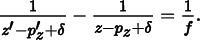
Lens systems can be focused at a given depth in the scene by moving the system in relation to the film so that a point at the desired focus depth images to a point on the film plane. The Gaussian lens equation, (6.3), gives us a relation that we can solve to focus a thick lens.
For thick lenses, the Gaussian lens equation relates distances from a point in the scene at z and the point it focuses to z′ by
For thin lenses, pz = pz′ = 0, and Equation (6.1) follows.
If we know the positions pz and pz′ of the principal planes and the focal length of the lens f and would like to focus at some depth z along the optical axis, then we need to determine how far to translate the system δ so that
The focal point on the film side should be at the film, so z′ = 0, and z = zf, the given focus depth. The only unknown is δ, and some algebraic manipulation gives us

(There are actually two solutions, but this one, which is the closer of the two, gives a small adjustment to the lens position and is thus the appropriate one.)
FocusThickLens() focuses the lens system using this approximation. After computing δ, it returns the offset along the z axis from the film where the lens system should be placed.
〈RealisticCamera Method Definitions〉 + ≡
Float RealisticCamera::FocusThickLens(Float focusDistance) {
Float pz[2], fz[2];
ComputeThickLensApproximation(pz, fz);
〈Compute translation of lens, delta, to focus at focusDistance 389〉
return elementInterfaces.back().thickness + delta;
}
Equation (6.4) gives the offset δ. The focal length of the lens f is the distance between the cardinal points fz′ and pz′. Note also that the negation of the focus distance is used for z, since the optical axis points along negative z.
〈Compute translation of lens, delta, to focus at focusDistance〉 ≡ 388
Float f = fz[0] - pz[0];
Float z = -focusDistance;
Float delta = 0.5f * (pz[1] - z + pz[0] -
std::sqrt((pz[1] - z - pz[0]) * (pz[1] - z - 4 * f - pz[0])));
We can now finally implement the fragment in the RealisticCamera constructor that focuses the lens system. (Recall that the thickness of the rearmost element interface is the distance from the interface to the film.)
〈Compute lens–film distance for given focus distance〉 ≡ 379
elementInterfaces.back().thickness = FocusThickLens(focusDistance);
6.4.5 The exit pupil
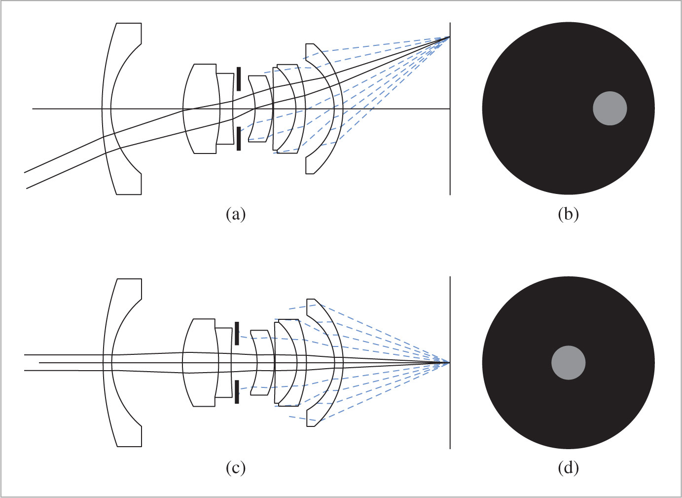
From a given point on the film plane, not all rays toward the rear lens element will successfully exit the lens system; some will be blocked by the aperture stop or will intersect the lens system enclosure. In turn, not all points on the rear lens element transmit radiance to the point on the film. The set of points on the rear element that do carry light through the lens system is called the exit pupil; its size and position vary across viewpoints on the film plane. (Analogously, the entrance pupil is the area over the front lens element where rays from a given point in the scene will reach the film.)
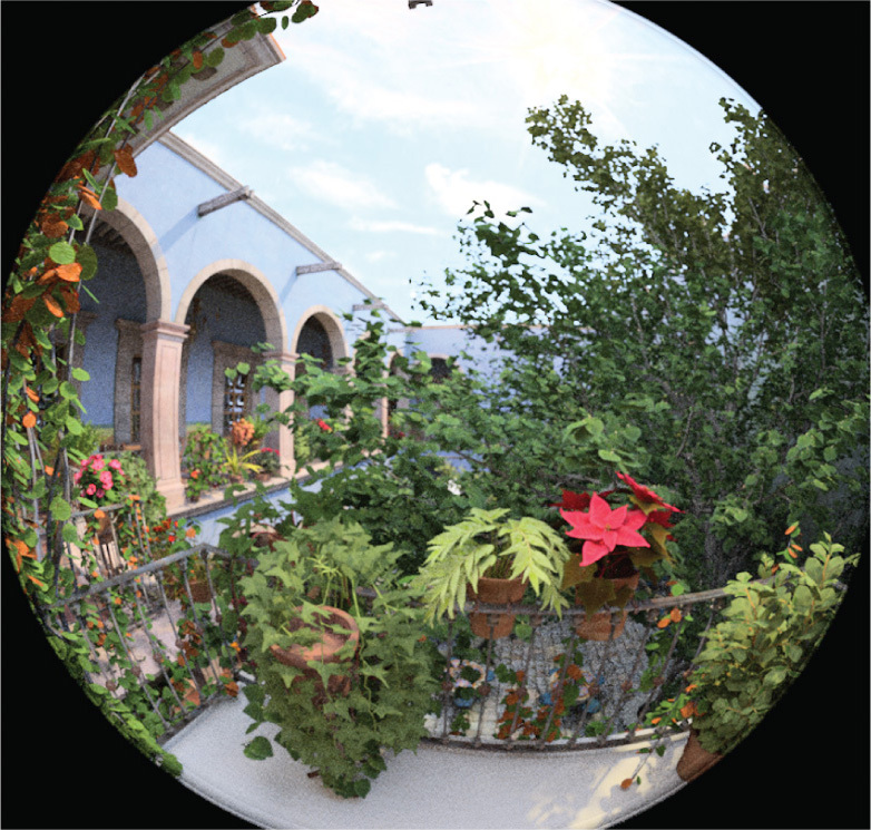
Figure 6.22 shows the exit pupil as seen from two points on the film plane with a wide angle lens. The exit pupil gets smaller for points toward the edges of the film. An implication of this shrinkage is vignetting.
When tracing rays starting from the film, we’d like to avoid tracing too many rays that don’t make it through the lens system; therefore, it’s worth limiting sampling to the exit pupil itself and a small area around it rather than, for example, wastefully sampling the entire area of the rear lens element.
Computing the exit pupil at each point on the film plane before tracing a ray would be prohibitively expensive; instead the RealisticCamera implementation precomputes exit pupil bounds along segments of a line on the film plane. Since we assumed that the lens system is radially symmetric around the optical axis, exit pupil bounds will also be radially symmetric, and bounds for arbitrary points on the film plane can be found by rotating these segment bounds appropriately (Figure 6.23). These bounds are then used to efficiently find exit pupil bounds for specific film sample positions.
One important subtlety to be aware of is that because the lens system is focused by translating it along the optical axis, the shape and position of the exit pupil change when the focus of the lens system is adjusted. Therefore, it’s critical that these bounds be computed after focusing.3
〈Compute exit pupil bounds at sampled points on the film〉 ≡ 379
int nSamples = 64;
exitPupilBounds.resize(nSamples);
ParallelFor(
[&](int i) {
Float r0 = (Float)i / nSamples * film- > diagonal / 2;
Float r1 = (Float)(i + 1) / nSamples * film- > diagonal / 2;
exitPupilBounds[i] = BoundExitPupil(r0, r1);
}, nSamples);
〈RealisticCamera Private Data〉 + ≡ 378
std::vector < Bounds2f > exitPupilBounds;
The BoundExitPupil() method computes a 2D bounding box of the exit pupil as seen from a point along a segment on the film plane. The bounding box is computed by attempting to trace rays through the lens system at a set of points on a plane tangent to the rear lens element. The bounding box of the rays that make it through the lens system gives an approximate bound on the exit pupil—see Figure 6.24.

〈RealisticCamera Method Definitions〉 + ≡
Bounds2f RealisticCamera::BoundExitPupil(Float pFilmX0,
Float pFilmX1) const {
Bounds2f pupilBounds;
〈Sample a collection of points on the rear lens to find exit pupil 392〉
〈Return entire element bounds if no rays made it through the lens system 393〉
〈Expand bounds to account for sample spacing 393〉
return pupilBounds;
}
The implementation samples the exit pupil fairly densely—at a total of 10242 points for each segment. We’ve found this sampling rate to provide good exit pupil bounds in practice.
〈Sample a collection of points on the rear lens to find exit pupil〉 ≡ 391
const int nSamples = 1024 * 1024;
int nExitingRays = 0;
〈Compute bounding box of projection of rear element on sampling plane 392〉
for (int i = 0; i < nSamples; ++i) {
〈Find location of sample points on x segment and rear lens element 392〉
〈Expand pupil bounds if ray makes it through the lens system 392〉
}
The bounding box of the rear element in the plane perpendicular to it is not enough to be a conservative bound of the projection of the exit pupil on that plane; because the element is generally curved, rays that pass through the plane outside of that bound may themselves intersect the valid extent of the rear lens element. Rather than compute a precise bound, we’ll increase the bounds substantially. The result is that many of the samples taken to compute the exit pupil bound will be wasted; in practice, this is a minor price to pay, as these samples are generally quickly terminated during the lens ray-tracing phase.
〈Compute bounding box of projection of rear element on sampling plane〉 ≡ 392
Float rearRadius = RearElementRadius();
Bounds2f projRearBounds(Point2f(-1.5f * rearRadius, -1.5f * rearRadius),
Point2f( 1.5f * rearRadius, 1.5f * rearRadius));
The x sample point on the film is found by linearly interpolating between the x interval endpoints. The RadicalInverse() function that is used to compute the interpolation offsets for the sample point inside the exit pupil bounding box will be defined later, in Section 7.4.1. There, we will see that the sampling strategy implemented here corresponds to using Hammersley points in 3D; the resulting point set minimizes gaps in the coverage of the overall 3D domain, which in turn ensures an accurate exit pupil bound estimate.
〈Find location of sample points on x segment and rear lens element〉 ≡ 392
Point3f pFilm(Lerp((i + 0.5f) / nSamples, pFilmX0, pFilmX1), 0, 0);
Float u[2] = { RadicalInverse(0, i), RadicalInverse(1, i) };
Point3f pRear(Lerp(u[0], projRearBounds.pMin.x, projRearBounds.pMax.x),
Lerp(u[1], projRearBounds.pMin.y, projRearBounds.pMax.y),
LensRearZ());
Now we can construct a ray from pFilm to pRear and determine if it is within the exit pupil by seeing if it makes it out of the front of the lens system. If so, the exit pupil bounds are expanded to include this point. If the sampled point is already inside the exit pupil’s bounding box as computed so far, then we can skip the lens ray tracing step to save a bit of unnecessary work.
〈Expand pupil bounds if ray makes it through the lens system〉 ≡ 392
if (Inside(Point2f(pRear.x, pRear.y), pupilBounds) ||
TraceLensesFromFilm(Ray(pFilm, pRear - pFilm), nullptr)) {
pupilBounds = Union(pupilBounds, Point2f(pRear.x, pRear.y));
++nExitingRays;
}
It may be that none of the sample rays makes it through the lens system; this case can legitimately happen with some very wide-angle lenses where the exit pupil vanishes at the edges of the film extent, for example. In this case, the bound doesn’t matter and BoundExitPupil() returns the bound that encompasses the entire rear lens element.
〈Return entire element bounds if no rays made it through the lens system〉 ≡ 391
if (nExitingRays == 0)
return projRearBounds;
While one sample may have made it through the lens system and one of its neighboring samples didn’t, it may well be that another sample very close to the neighbor actually would have made it out. Therefore, the final bound is expanded by roughly the spacing between samples in each direction in order to account for this uncertainty.
〈Expand bounds to account for sample spacing〉 ≡ 391
pupilBounds = Expand(pupilBounds,
2 * projRearBounds.Diagonal().Length() /
std::sqrt(nSamples));
Given the precomputed bounds stored in RealisticCamera::exitPupilBounds, the SampleExitPupil() method can fairly efficiently find the bounds on the exit pupil for a given point on the film plane. It then samples a point inside this bounding box for the ray from the film to pass through. In order to accurately model the radiometry of image formation, the following code will need to know the area of this bounding box, so it is returned via sampleBoundsArea.
〈RealisticCamera Method Definitions〉 + ≡
Point3f RealisticCamera::SampleExitPupil(const Point2f &pFilm,
const Point2f &lensSample, Float *sampleBoundsArea) const {
〈Find exit pupil bound for sample distance from film center 393〉
〈Generate sample point inside exit pupil bound 393〉
〈Return sample point rotated by angle of pFilm with + x axis 394〉
}
〈Find exit pupil bound for sample distance from film center〉 ≡ 393
Float rFilm = std::sqrt(pFilm.x * pFilm.x + pFilm.y * pFilm.y);
int rIndex = rFilm / (film- > diagonal / 2) * exitPupilBounds.size();
rIndex = std::min((int)exitPupilBounds.size() - 1, rIndex);
Bounds2f pupilBounds = exitPupilBounds[rIndex];
if (sampleBoundsArea) *sampleBoundsArea = pupilBounds.Area();
Given the pupil’s bounding box, a point inside it is sampled via linear interpolation with the provided lensSample value, which is in [0, 1)2.
〈Generate sample point inside exit pupil bound〉 ≡ 393
Point2f pLens = pupilBounds.Lerp(lensSample);
Because the exit pupil bound was computed from a point on the film along the + x axis but the point pFilm is an arbitrary point on the film, the sample point in the exit pupil bound must be rotated by the same angle as pFilm makes with the + x axis.
〈Return sample point rotated by angle of pFilm with + x axis〉 ≡ 393
Float sinTheta = (rFilm ! = 0) ? pFilm.y / rFilm : 0;
Float cosTheta = (rFilm ! = 0) ? pFilm.x / rFilm : 1;
return Point3f(cosTheta * pLens.x - sinTheta * pLens.y,
sinTheta * pLens.x + cosTheta * pLens.y,
LensRearZ());
6.4.6 Generating rays
Now that we have the machinery to trace rays through lens systems and to sample points in the exit pupil bound from points on the film plane, transforming a CameraSample into a ray leaving the camera is fairly straightforward: we need to compute the sample’s position on the film plane and generate a ray from this point to the rear lens element, which is then traced through the lens system.
〈RealisticCamera Method Definitions〉 + ≡
Float RealisticCamera::GenerateRay(const CameraSample &sample,
Ray *ray) const {
〈Find point on film, pFilm , corresponding to sample.pFilm 394〉
〈Trace ray from pFilm through lens system 394〉
〈Finish initialization of RealisticCamera ray 395〉
〈Return weighting for RealisticCamera ray 783〉
}
The CameraSample::pFilm value is with respect to the overall resolution of the image in pixels. Here, we’re operating with a physical model of a sensor, so we start by converting back to a sample in [0, 1)2. Next, the corresponding point on the film is found by linearly interpolating with this sample value over its area.
〈Find point on film, pFilm, corresponding to sample.pFilm〉 ≡ 394
Point2f s(sample.pFilm.x / film- > fullResolution.x,
sample.pFilm.y / film- > fullResolution.y);
Point2f pFilm2 = film- > GetPhysicalExtent().Lerp(s);
Point3f pFilm(-pFilm2.x, pFilm2.y, 0);
SampleExitPupil() then gives us a point on the plane tangent to the rear lens element, which in turn lets us determine the ray’s direction. In turn, we can trace this ray through the lens system. If the ray is blocked by the aperture stop or otherwise doesn’t make it through the lens system, GenerateRay() returns a 0 weight. (Callers should be sure to check for this case.)
〈Trace ray from pFilm through lens system〉 ≡ 394
Float exitPupilBoundsArea;
Point3f pRear = SampleExitPupil(Point2f(pFilm.x, pFilm.y), sample.pLens,
&exitPupilBoundsArea);
Ray rFilm(pFilm, pRear - pFilm, Infinity,
Lerp(sample.time, shutterOpen, shutterClose));
if (!TraceLensesFromFilm(rFilm, ray))
return 0;
If the ray does successfully exit the lens system, then the usual details have to be handled to finish its initialization.
〈Finish initialization of RealisticCamera ray〉 ≡ 394
*ray = CameraToWorld(*ray);
ray- > d = Normalize(ray- > d);
ray- > medium = medium;
The fragment 〈Return weighting for RealisticCamera ray〉 will be defined later, in Section 13.6.6, after some necessary background from Monte Carlo integration has been introduced.
6.4.7 The camera measurement equation
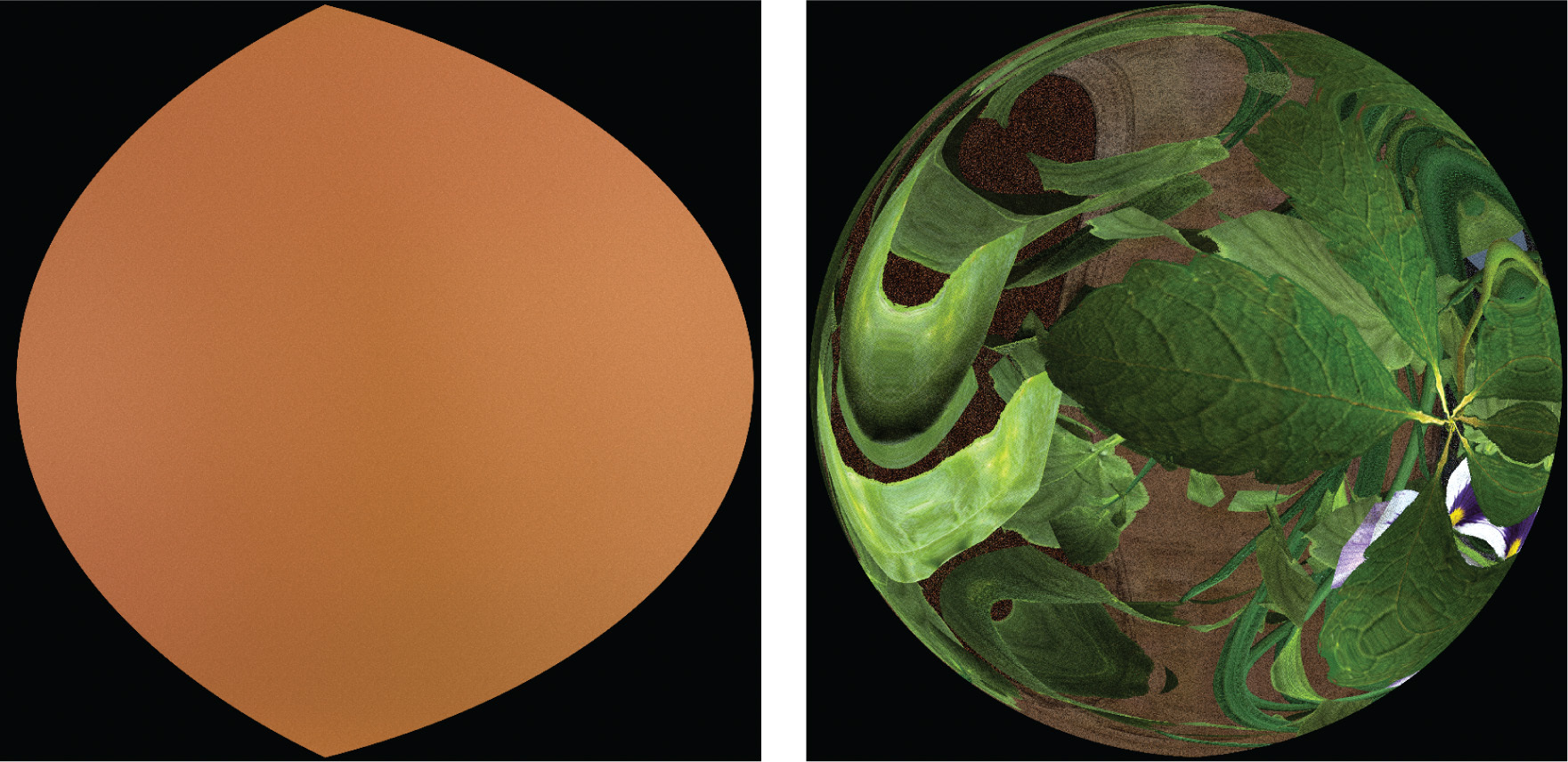
Given this more accurate simulation of the process of real image formation, it’s also worthwhile to more carefully define the radiometry of the measurement made by a film or a camera sensor. Rays from the exit pupil to the film carry radiance from the scene; as considered from a point on the film plane, there is thus a set of directions from which radiance is incident. The distribution of radiance leaving the exit pupil is affected by the amount of defocus blur seen by the point on the film—Figure 6.25 shows two renderings of the exit pupil’s radiance as seen from two points on the film.
Given the incident radiance function, we can define the irradiance at a point on the film plane. If we start with the definition of irradiance in terms of radiance, Equation (5.4), we can then convert from an integral over solid angle to an integral over area (in this case, an area of the plane tangent to the rear lens element that bounds the exit pupil, Ae) using Equation (5.6). This gives us the irradiance for a point p on the film plane:
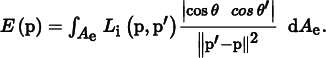
Figure 6.26 shows the geometry of the situation. Because the film plane is perpendicular to the exit pupil plane, θ = θ′. We can further take advantage of the fact that the distance between p and p′ is equal to the axial distance from the film plane to the exit pupil (which we’ll denote here by z) times cos θ. Putting this all together, we have
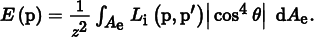
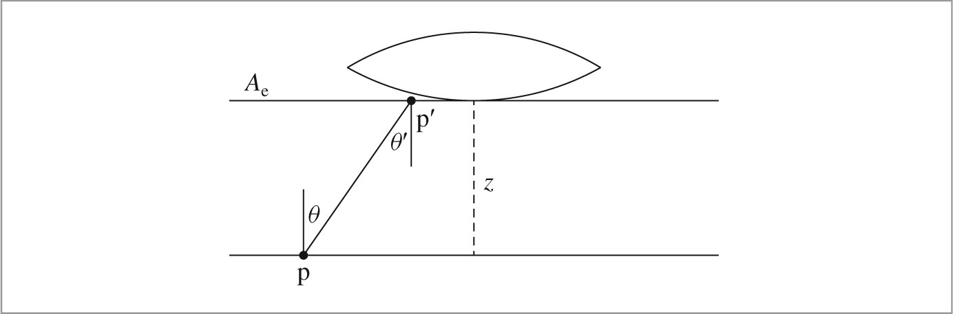
For cameras where the extent of the film is relatively large with respect to the distance z, the cos4θ term can meaningfully reduce the incident irradiance—this factor also contributes to vignetting. Most modern digital cameras correct for this effect with preset correction factors that increase pixel values toward the edges of the sensor.
Integrating irradiance at a point on the film over the time that the shutter is open gives fluence, which is the radiometric unit for energy per area, J/m2.

Measuring fluence at a point captures the effect that the amount of energy received on the film plane is partially related to the length of time the camera shutter is open.
Photographic film (or CCD or CMOS sensors in digital cameras) actually measure radiant energy over a small area.4 Taking Equation (6.6) and also integrating over sensor pixel area, Ap, we have

the Joules arriving at a pixel.
In Section 13.2, we’ll see how Monte Carlo can be applied to estimate the values of these various integrals. Then in Section 13.6.6 we will define the fragment 〈Return weighting for RealisticCamera ray〉 in RealisticCamera::GenerateRay(); various approaches to computing the weight allow us to compute each of these quantities. Section 16.1.1 defines the importance function of a camera model, which characterizes its sensitivity to incident illumination arriving along different rays.
Further reading
In his seminal Sketchpad system, Sutherland (1963) was the first to use projection matrices for computer graphics. Akenine-Möller, Haines, and Hoffman (2008) have provided a particularly well-written derivation of the orthographic and perspective projection matrices. Other good references for projections are Rogers and Adams’s Mathematical Elements for Computer Graphics (1990), and Eberly’s book (2001) on game engine design.
An unusual projection method was used by Greene and Heckbert (1986) for generating images for Omnimax® theaters. The EnvironmentCamera in this chapter is similar to the camera model described by Musgrave (1992).
Potmesil and Chakravarty (1981, 1982, 1983) did early work on depth of field and motion blur in computer graphics. Cook and collaborators developed a more accurate model for these effects based on the thin lens model; this is the approach used for the depth of field calculations in Section 6.2.3 (Cook, Porter, and Carpenter 1984; Cook 1986). See Adams and Levoy (2007) for a broad analysis of the types of radiance measurements that can be taken with cameras that have non-pinhole apertures.
Kolb, Mitchell, and Hanrahan (1995) showed how to simulate complex camera lens systems with ray tracing in order to model the imaging effects of real cameras; the RealisticCamera in Section 6.4 is based on their approach. Steinert et al. (2011) improve a number of details of this simulation, incorporating wavelength-dependent effects and accounting for both diffraction and glare. Our approach for approximating the exit pupil in Section 6.4.5 is similar to theirs. See the books by Hecht (2002) and Smith (2007) for excellent introductions to optics and lens systems.
Hullin et al. (2012) use polynomials to model the effect of lenses on rays passing through them; they are able to construct polynomials that approximate entire lens systems from polynomial approximations of individual lenses. This approach saves the computational expense of tracing rays through lenses, though for complex scenes, this cost is generally negligible in relation to the rest of rendering computations. Hanika and Dachsbacher (2014) improved the accuracy of this approach and showed how to combine the method with bidirectional path tracing.
Chen et al. (2009) describe the implementation a fairly complete simulation of a digital camera, including the analog-to-digital conversion and noise in the measured pixel values inherent in this process.
Exercises
 6.1 Some types of cameras expose the film by sliding a rectangular slit across the film. This leads to interesting effects when objects are moving in a different direction from the exposure slit (Glassner 1999; Stephenson 2006). Furthermore, most digital cameras read out pixel values from scanlines in succession over a period of a few milliseconds; this leads to rolling shutter artifacts, which have similar visual characteristics. Modify the way that time samples are generated in one or more of the camera implementations in this chapter to model such effects. Render images with moving objects that clearly show the effect of accounting for this issue.
6.2 Write an application that loads images rendered by the EnvironmentCamera, and uses texture mapping to apply them to a sphere centered at the eyepoint such that they can be viewed interactively. The user should be able to freely change the viewing direction. If the correct texture-mapping function is used for generating texture coordinates on the sphere, the image generated by the application will appear as if the viewer was at the camera’s location in the scene when it was rendered, thus giving the user the ability to interactively look around the scene.
6.3 The aperture stop in the RealisticCamera is modeled as a perfect circle; for cameras with adjustable apertures, the aperture is generally formed by movable blades with straight edges and is thus an n-gon. Modify the RealisticCamera to model a more realistic aperture shape and render images showing the differences from your model. You may find it useful to render a scene with small, bright, out-of-focus objects (e.g., specular highlights), to show off the differences.
6.4 The standard model for depth of field in computer graphics models the circle of confusion as imaging a point in the scene to a disk with uniform intensity, although many real lenses produce circles of confusion with nonlinear variation such as a Gaussian distribution. This effect is known as “Bokeh” (Buhler and Wexler 2002). For example, catadioptric (mirror) lenses produce doughnut-shaped highlights when small points of light are viewed out of focus. Modify the implementation of depth of field in the RealisticCamera to produce images with this effect (e.g., by biasing the distribution of lens sample positions). Render images showing the difference between this and the standard model.
6.5 Focal stack rendering: a focal stack is a series of images of a fixed scene where the camera is focused at a different distance for each image. Hasinoff and Kutulakos (2011) and Jacobs et al. (2012) introduce a number of applications of focal stacks, including freeform depth of field, where the user can specify arbitrary depths that are in focus, achieving effects not possible with traditional optics. Render focal stacks with pbrt and write an interactive tool to control focus effects with them.
 6.6 Light field camera: Ng et al. (2005) discuss the physical design and applications of a camera that captures small images of the exit pupil across the film, rather than averaging the radiance over the entire exit pupil at each pixel, as conventional cameras do. Such a camera captures a representation of the light field—the spatially and directionally varying distribution of radiance arriving at the camera sensor. By capturing the light field, a number of interesting operations are possible, including refocusing photographs after they have been taken. Read Ng et al.’s paper and implement a Camera in pbrt that captures the light field of a scene. Write a tool to allow users to interactively refocus these light fields.
6.7 The RealisticCamera implementation places the film at the center of and perpendicular to the optical axis. While this is the most common configuration of actual cameras, interesting effects can be achieved by adjusting the film’s placement with respect to the lens system.
For example, the plane of focus in the current implementation is always perpendicular to the optical axis; if the film plane (or the lens system) is tilted so that the film isn’t perpendicular to the optical axis, then the plane of focus is no longer perpendicular to the optical axis. (This can be useful for landscape photography, for example, where aligning the plane of focus with the ground plane allows greater depth of field even with larger apertures.) Alternatively, the film plane can be shifted so that it’s not centered on the optical axis; this shift can be used to keep the plane of focus aligned with a very tall object, for example.
Modify RealisticCamera to allow one or both of these adjustments and render images showing the result. Note that a number of places in the current implementation (e.g., the exit pupil computation) have assumptions that will be violated by these changes that you will need to address.