Sampling and Reconstruction
Although the final output of a renderer like pbrt is a 2D grid of colored pixels, incident radiance is actually a continuous function defined over the film plane. The manner in which the discrete pixel values are computed from this continuous function can noticeably affect the quality of the final image generated by the renderer; if this process is not performed carefully, artifacts will be present. Conversely, if it is performed well, a relatively small amount of additional computation to this end can substantially improve the quality of the rendered images.
This chapter starts by introducing sampling theory—the theory of taking discrete sample values from functions defined over continuous domains and then using those samples to reconstruct new functions that are similar to the original. Building on principles of sampling theory as well as ideas from low-discrepancy point sets, which are a particular type of well-distributed sample points, the Samplers defined in this chapter generate n-dimensional sample vectors in various ways.1 Five Sampler implementations are described in this chapter, spanning a variety of approaches to the sampling problem.
This chapter concludes with the Filter class and the Film class. The Filter is used to determine how multiple samples near each pixel are blended together to compute the final pixel value, and the Film class accumulates image sample contributions into pixels of images.
7.1 Sampling theory
A digital image is represented as a set of pixel values, typically aligned on a rectangular grid. When a digital image is displayed on a physical device, these values are used to determine the spectral power emitted by pixels on the display. When thinking about digital images, it is important to differentiate between image pixels, which represent the value of a function at a particular sample location, and display pixels, which are physical objects that emit light with some distribution. (For example, in an LCD display, the color and brightness may change substantially when the display is viewed at oblique angles.) Displays use the image pixel values to construct a new image function over the display surface. This function is defined at all points on the display, not just the infinitesimal points of the digital image’s pixels. This process of taking a collection of sample values and converting them back to a continuous function is called reconstruction.
In order to compute the discrete pixel values in the digital image, it is necessary to sample the original continuously defined image function. In pbrt, like most other ray-tracing renderers, the only way to get information about the image function is to sample it by tracing rays. For example, there is no general method that can compute bounds on the variation of the image function between two points on the film plane. While an image could be generated by just sampling the function precisely at the pixel positions, a better result can be obtained by taking more samples at different positions and incorporating this additional information about the image function into the final pixel values. Indeed, for the best quality result, the pixel values should be computed such that the reconstructed image on the display device is as close as possible to the original image of the scene on the virtual camera’s film plane. Note that this is a subtly different goal from expecting the display’s pixels to take on the image function’s actual value at their positions. Handling this difference is the main goal of the algorithms implemented in this chapter.2
Because the sampling and reconstruction process involves approximation, it introduces error known as aliasing, which can manifest itself in many ways, including jagged edges or flickering in animations. These errors occur because the sampling process is not able to capture all of the information from the continuously defined image function.
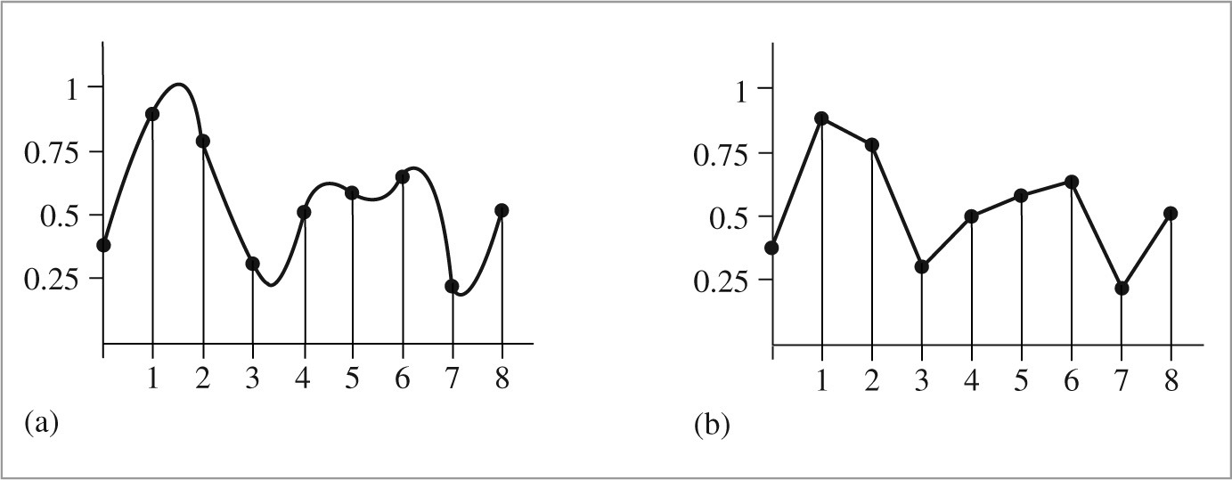
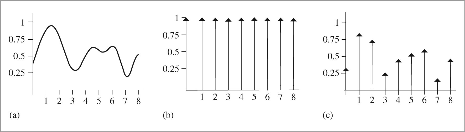
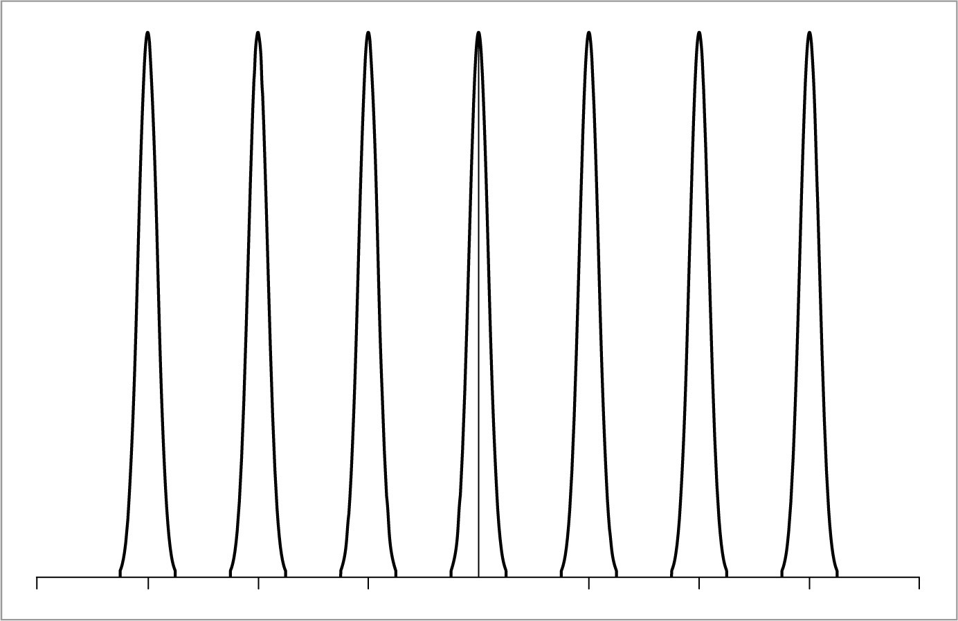
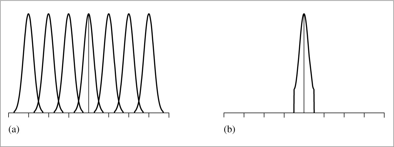
As an example of these ideas, consider a 1D function (which we will interchangeably refer to as a signal), given by f (x), where we can evaluate f (x′) at any desired location x′ in the function’s domain. Each such x′ is called a sample position, and the value of f (x′) is the sample value. Figure 7.1 shows a set of samples of a smooth 1D function, along with a reconstructed signal  that approximates the original function f. In this example, is a piecewise linear function that approximates f by linearly interpolating neighboring sample values (readers already familiar with sampling theory will recognize this as reconstruction with a hat function). Because the only information available about f comes from the sample values at the positions x′, is unlikely to match f perfectly since there is no information about f ’s behavior between the samples.

that is an approximation to f (x). The sampling theorem, introduced in Section 7.1.3, makes a precise statement about the conditions on f (x), the number of samples taken, and the reconstruction technique used under which
is exactly the same as f (x). The fact that the original function can sometimes be reconstructed exactly from point samples alone is remarkable.
Fourier analysis can be used to evaluate the quality of the match between the reconstructed function and the original. This section will introduce the main ideas of Fourier analysis with enough detail to work through some parts of the sampling and reconstruction processes but will omit proofs of many properties and skip details that aren’t directly relevant to the sampling algorithms used in pbrt. The “Further Reading” section of this chapter has pointers to more detailed information about these topics.
7.1.1 The frequency domain and the fourier transform
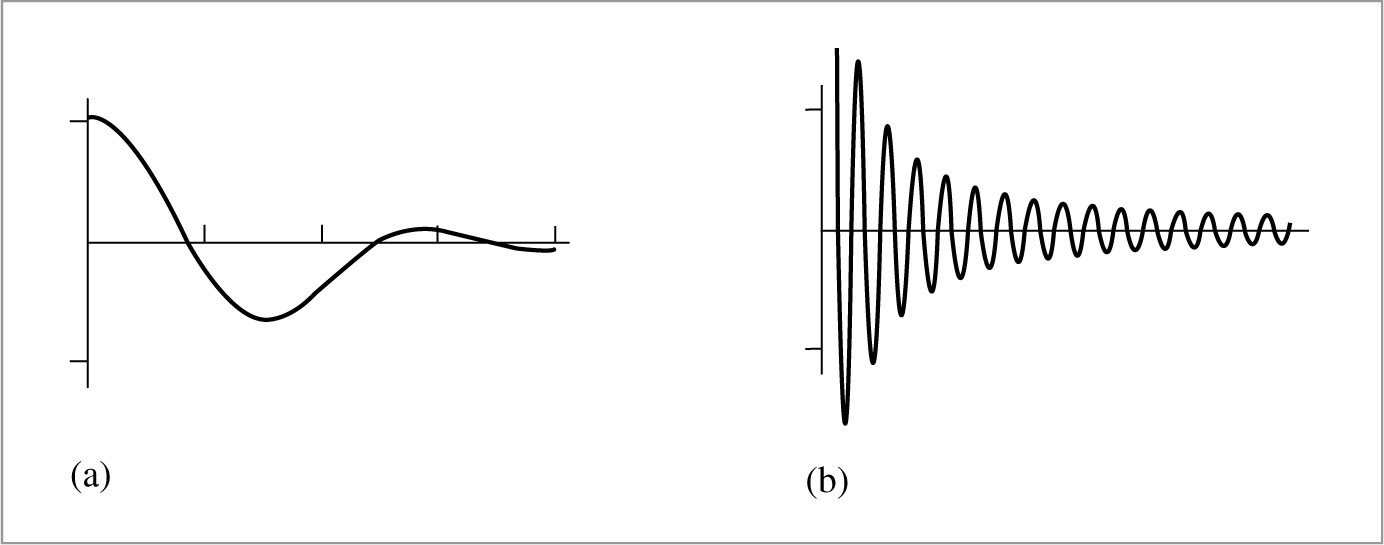
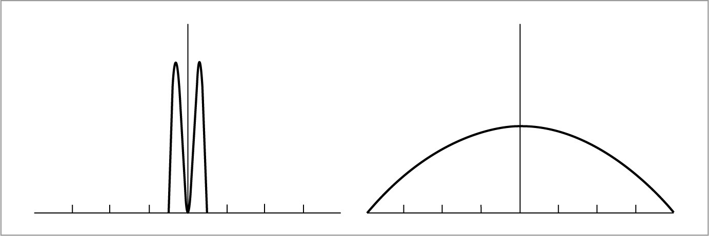
One of the foundations of Fourier analysis is the Fourier transform, which represents a function in the frequency domain. (We will say that functions are normally expressed in the spatial domain.) Consider the two functions graphed in Figure 7.2. The function in Figure 7.2(a) varies relatively slowly as a function of x, while the function in Figure 7.2(b) varies much more rapidly. The more slowly varying function is said to have lower frequency content. Figure 7.3 shows the frequency space representations of these two functions; the lower frequency function’s representation goes to 0 more quickly than does the higher frequency function.
Most functions can be decomposed into a weighted sum of shifted sinusoids. This remarkable fact was first described by Joseph Fourier, and the Fourier transform converts a function into this representation. This frequency space representation of a function gives insight into some of its characteristics—the distribution of frequencies in the sine functions corresponds to the distribution of frequencies in the original function. Using this form, it is possible to use Fourier analysis to gain insight into the error that is introduced by the sampling and reconstruction process and how to reduce the perceptual impact of this error.
The Fourier transform of a 1D function f (x) is3
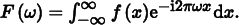
(Recall that eix = cos x + i sin x, where  .) For simplicity, here we will consider only even functions where f (− x) = f (x), in which case the Fourier transform of f has no imaginary terms. The new function F is a function of frequency, ω.4 We will denote the Fourier transform operator by
  , such that
  . is clearly a linear operator—that is,
  for any scalar a, and
  .
.
Equation (7.1) is called the Fourier analysis equation, or sometimes just the Fourier transform. We can also transform from the frequency domain back to the spatial domain using the Fourier synthesis equation, or the inverse Fourier transform:
Table 7.1 shows a number of important functions and their frequency space representations. A number of these functions are based on the Dirac delta distribution, a special function that is defined such that  , and for all x ≠ 0, δ(x) = 0. An important consequence of these properties is that
Table 7.1
Fourier Pairs. Functions in the spatial domain and their frequency space representations. Because of the symmetry properties of the Fourier transform, if the left column is instead considered to be frequency space, then the right column is the spatial equivalent of those functions as well.
| Spatial Domain | Frequency Space Representation |
| Box: f (x) = 1 if |x| < 1/2, 0 otherwise | Sinc: f (ω) = sinc(ω) = sin(πω)/(πω) |
Gaussian:  | Gaussian:  |
| Constant: f (x) = 1 | Delta: f (ω) = δ(ω) |
| Sinusoid: f (x) = cos x | Translated delta: f (ω) = π(δ(1 − 2πω) + δ(1 + 2πω)) |
| Shah: f (x) = ШT(x) = T ∑iδ(x − Ti) | Shah: f (ω) = Ш1/T(ω) = (1/T) ∑iδ(ω − i/T) |
The delta distribution cannot be expressed as a standard mathematical function, but instead is generally thought of as the limit of a unit area box function centered at the origin with width approaching 0.
7.1.2 Ideal sampling and reconstruction
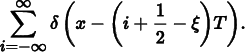
Using frequency space analysis, we can now formally investigate the properties of sampling. Recall that the sampling process requires us to choose a set of equally spaced sample positions and compute the function’s value at those positions. Formally, this corresponds to multiplying the function by a “shah,” or “impulse train,” function, an infinite sum of equally spaced delta functions. The shah ШT (x) is defined as
where T defines the period, or sampling rate. This formal definition of sampling is illustrated in Figure 7.4. The multiplication yields an infinite sequence of values of the function at equally spaced points:

These sample values can be used to define a reconstructed function by choosing a reconstruction filter function r(x) and computing the convolution
where the convolution operation ⊗ is defined as

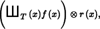
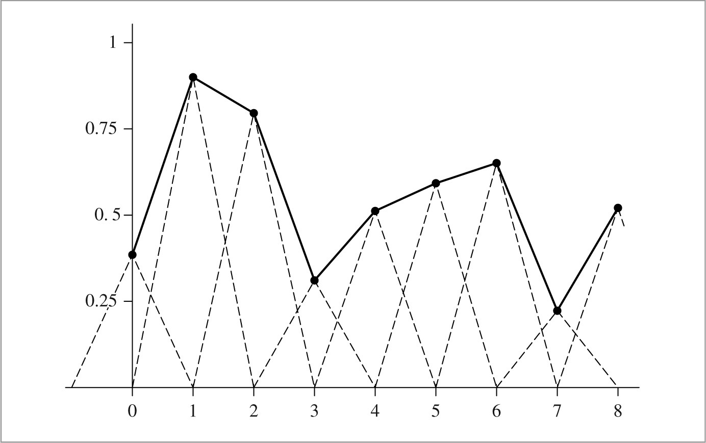
For reconstruction, convolution gives a weighted sum of scaled instances of the reconstruction filter centered at the sample points:
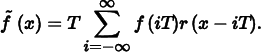
For example, in Figure 7.1, the triangle reconstruction filter, r(x) = max(0, 1 − |x|), was used. Figure 7.5 shows the scaled triangle functions used for that example.
We have gone through a process that may seem gratuitously complex in order to end up at an intuitive result: the reconstructed function can be obtained by interpolating among the samples in some manner. By setting up this background carefully, however, Fourier analysis can now be applied to the process more easily.
We can gain a deeper understanding of the sampling process by analyzing the sampled function in the frequency domain. In particular, we will be able to determine the conditions under which the original function can be exactly recovered from its values at the sample locations—a very powerful result. For the discussion here, we will assume for now that the function f (x) is band limited—there exists some frequency ω0 such that f (x) contains no frequencies greater than ω0. By definition, band-limited functions have frequency space representations with compact support, such that F (ω) = 0 for all |ω| > ω0. Both of the spectra in Figure 7.3 are band limited.
An important idea used in Fourier analysis is the fact that the Fourier transform of the product of two functions  can be shown to be the convolution of their individual Fourier transforms F (ω) and G(ω):

It is similarly the case that convolution in the spatial domain is equivalent to multiplication in the frequency domain:

These properties are derived in the standard references on Fourier analysis. Using these ideas, the original sampling step in the spatial domain, where the product of the shah function and the original function f (x) is found, can be equivalently described by the convolution of F (ω) with another shah function in frequency space.
We also know the spectrum of the shah function ШT(x) from Table 7.1; the Fourier transform of a shah function with period T is another shah function with period 1/T. This reciprocal relationship between periods is important to keep in mind: it means that if the samples are farther apart in the spatial domain, they are closer together in the frequency domain.
Thus, the frequency domain representation of the sampled signal is given by the convolution of F (ω) and this new shah function. Convolving a function with a delta function just yields a copy of the function, so convolving with a shah function yields an infinite sequence of copies of the original function, with spacing equal to the period of the shah (Figure 7.6). This is the frequency space representation of the series of samples.
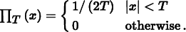
Now that we have this infinite set of copies of the function’s spectrum, how do we reconstruct the original function? Looking at Figure 7.6, the answer is obvious: just discard all of the spectrum copies except the one centered at the origin, giving the original F (ω). In order to throw away all but the center copy of the spectrum, we multiply by a box function of the appropriate width (Figure 7.7). The box function ΠT (x) of width T is defined as
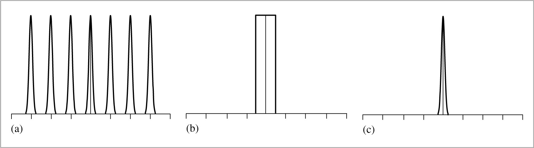
This multiplication step corresponds to convolution with the reconstruction filter in the spatial domain. This is the ideal sampling and reconstruction process. To summarize:

This is a remarkable result: we have been able to determine the exact frequency space representation of f (x), purely by sampling it at a set of regularly spaced points. Other than knowing that the function was band limited, no additional information about the composition of the function was used.
Applying the equivalent process in the spatial domain will likewise recover f (x) exactly. Because the inverse Fourier transform of the box function is the sinc function, ideal reconstruction in the spatial domain is
or

Unfortunately, because the sinc function has infinite extent, it is necessary to use all of the sample values f (i) to compute any particular value of in the spatial domain. Filters with finite spatial extent are preferable for practical implementations even though they don’t reconstruct the original function perfectly.
A commonly used alternative in graphics is to use the box function for reconstruction, effectively averaging all of the sample values within some region around x. This is a very poor choice, as can be seen by considering the box filter’s behavior in the frequency domain: This technique attempts to isolate the central copy of the function’s spectrum by multiplying by a sinc, which not only does a bad job of selecting the central copy of the function’s spectrum but includes high-frequency contributions from the infinite series of other copies of it as well.
7.1.3 Aliasing
Beyond the issue of the sinc function’s infinite extent, one of the most serious practical problems with the ideal sampling and reconstruction approach is the assumption that the signal is band limited. For signals that are not band limited, or signals that aren’t sampled at a sufficiently high sampling rate for their frequency content, the process described earlier will reconstruct a function that is different from the original signal.
The key to successful reconstruction is the ability to exactly recover the original spectrum F (ω) by multiplying the sampled spectrum with a box function of the appropriate width. Notice that in Figure 7.6, the copies of the signal’s spectrum are separated by empty space, so perfect reconstruction is possible. Consider what happens, however, if the original function was sampled with a lower sampling rate. Recall that the Fourier transform of a shah function ШT with period T is a new shah function with period 1/T. This means that if the spacing between samples increases in the spatial domain, the sample spacing decreases in the frequency domain, pushing the copies of the spectrum F (ω) closer together. If the copies get too close together, they start to overlap.
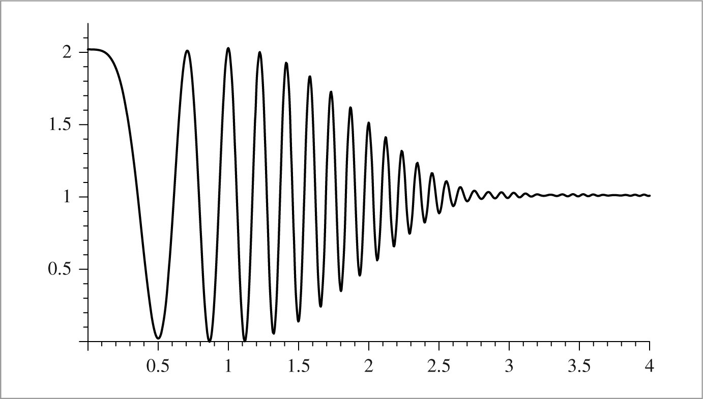
Because the copies are added together, the resulting spectrum no longer looks like many copies of the original (Figure 7.8). When this new spectrum is multiplied by a box function, the result is a spectrum that is similar but not equal to the original F (ω): high-frequency details in the original signal leak into lower frequency regions of the spectrum of the reconstructed signal. These new low-frequency artifacts are called aliases (because high frequencies are “masquerading” as low frequencies), and the resulting signal is said to be aliased. Figure 7.9 shows the effects of aliasing from undersampling and then reconstructing the 1D function f (x) = 1 + cos(4x2).

A possible solution to the problem of overlapping spectra is to simply increase the sampling rate until the copies of the spectrum are sufficiently far apart to not overlap, thereby eliminating aliasing completely. In fact, the sampling theorem tells us exactly what rate is required. This theorem says that as long as the frequency of uniform sample points ωs is greater than twice the maximum frequency present in the signal ω0, it is possible to reconstruct the original signal perfectly from the samples. This minimum sampling frequency is called the Nyquist frequency.
For signals that are not band limited (ω0 = ∞), it is impossible to sample at a high enough rate to perform perfect reconstruction. Non-band-limited signals have spectra with infinite support, so no matter how far apart the copies of their spectra are (i.e., how high a sampling rate we use), there will always be overlap. Unfortunately, few of the interesting functions in computer graphics are band limited. In particular, any function containing a discontinuity cannot be band limited, and therefore we cannot perfectly sample and reconstruct it. This makes sense because the function’s discontinuity will always fall between two samples and the samples provide no information about the location of the discontinuity. Thus, it is necessary to apply different methods besides just increasing the sampling rate in order to counteract the error that aliasing can introduce to the renderer’s results.
7.1.4 Antialiasing techniques
If one is not careful about sampling and reconstruction, myriad artifacts can appear in the final image. It is sometimes useful to distinguish between artifacts due to sampling and those due to reconstruction; when we wish to be precise we will call sampling artifacts prealiasing and reconstruction artifacts postaliasing. Any attempt to fix these errors is broadly classified as antialiasing. This section reviews a number of antialiasing techniques beyond just increasing the sampling rate everywhere.
Nonuniform Sampling
Although the image functions that we will be sampling are known to have infinite-frequency components and thus can’t be perfectly reconstructed from point samples, it is possible to reduce the visual impact of aliasing by varying the spacing between samples in a nonuniform way. If ξ denotes a random number between 0 and 1, a nonuniform set of samples based on the impulse train is
For a fixed sampling rate that isn’t sufficient to capture the function, both uniform and nonuniform sampling produce incorrect reconstructed signals. However, nonuniform sampling tends to turn the regular aliasing artifacts into noise, which is less distracting to the human visual system. In frequency space, the copies of the sampled signal end up being randomly shifted as well, so that when reconstruction is performed the result is random error rather than coherent aliasing.
Adaptive Sampling
Another approach that has been suggested to combat aliasing is adaptive supersampling: if we can identify the regions of the signal with frequencies higher than the Nyquist limit, we can take additional samples in those regions without needing to incur the computational expense of increasing the sampling frequency everywhere. It can be difficult to get this approach to work well in practice, because finding all of the places where supersampling is needed is difficult. Most techniques for doing so are based on examining adjacent sample values and finding places where there is a significant change in value between the two; the assumption is that the signal has high frequencies in that region.
In general, adjacent sample values cannot tell us with certainty what is really happening between them: even if the values are the same, the functions may have huge variation between them. Alternatively, adjacent samples may have substantially different values without any aliasing actually being present. For example, the texture-filtering algorithms in Chapter 10 work hard to eliminate aliasing due to image maps and procedural textures on surfaces in the scene; we would not want an adaptive sampling routine to needlessly take extra samples in an area where texture values are changing quickly but no excessively high frequencies are actually present.
Prefiltering
Another approach to eliminating aliasing that sampling theory offers is to filter (i.e., blur) the original function so that no high frequencies remain that can’t be captured accurately at the sampling rate being used. This approach is applied in the texture functions of Chapter 10. While this technique changes the character of the function being sampled by removing information from it, blurring is generally less objectionable than aliasing.
Recall that we would like to multiply the original function’s spectrum with a box filter with width chosen so that frequencies above the Nyquist limit are removed. In the spatial domain, this corresponds to convolving the original function with a sinc filter,

In practice, we can use a filter with finite extent that works well. The frequency space representation of this filter can help clarify how well it approximates the behavior of the ideal sinc filter.
Figure 7.10 shows the function 1 + cos(4x2) convolved with a variant of the sinc with finite extent that will be introduced in Section 7.8. Note that the high-frequency details have been eliminated; this function can be sampled and reconstructed at the sampling rate used in Figure 7.9 without aliasing.
7.1.5 Application to image synthesis
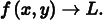
The application of these ideas to the 2D case of sampling and reconstructing images of rendered scenes is straightforward: we have an image, which we can think of as a function of 2D (x, y) image locations to radiance values L:
The good news is that, with our ray tracer, we can evaluate this function at any (x, y) point that we choose. The bad news is that it’s not generally possible to prefilter f to remove the high frequencies from it before sampling. Therefore, the samplers in this chapter will use both strategies of increasing the sampling rate beyond the basic pixel spacing in the final image as well as nonuniformly distributing the samples to turn aliasing into noise.
It is useful to generalize the definition of the scene function to a higher dimensional function that also depends on the time t and (u, v) lens position at which it is sampled. Because the rays from the camera are based on these five quantities, varying any of them gives a different ray and thus a potentially different value of f. For a particular image position, the radiance at that point will generally vary across both time (if there are moving objects in the scene) and position on the lens (if the camera has a finite-aperture lens).
Even more generally, because many of the integrators defined in Chapters 14 through 16 use statistical techniques to estimate the radiance along a given ray, they may return a different radiance value when repeatedly given the same ray. If we further extend the scene radiance function to include sample values used by the integrator (e.g., values used to choose points on area light sources for illumination computations), we have an even higher dimensional image function

Sampling all of these dimensions well is an important part of generating high-quality imagery efficiently. For example, if we ensure that nearby (x, y) positions on the image tend to have dissimilar (u, v) positions on the lens, the resulting rendered images will have less error because each sample is more likely to account for information about the scene that its neighboring samples do not. The Sampler classes in the next few sections will address the issue of sampling all of these dimensions effectively.
7.1.6 Sources of aliasing in rendering
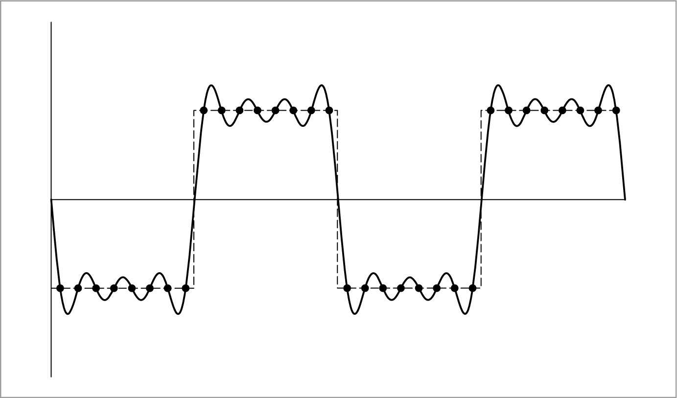
Geometry is one of the most common causes of aliasing in rendered images. When projected onto the image plane, an object’s boundary introduces a step function—the image function’s value instantaneously jumps from one value to another. Not only do step functions have infinite frequency content as mentioned earlier, but, even worse, the perfect reconstruction filter causes artifacts when applied to aliased samples: ringing artifacts appear in the reconstructed function, an effect known as the Gibbs phenomenon. Figure 7.11 shows an example of this effect for a 1D function. Choosing an effective reconstruction filter in the face of aliasing requires a mix of science, artistry, and personal taste, as we will see later in this chapter.
Very small objects in the scene can also cause geometric aliasing. If the geometry is small enough that it falls between samples on the image plane, it can unpredictably disappear and reappear over multiple frames of an animation.
Another source of aliasing can come from the texture and materials on an object. Shading aliasing can be caused by texture maps that haven’t been filtered correctly (addressing this problem is the topic of much of Chapter 10) or from small highlights on shiny surfaces. If the sampling rate is not high enough to sample these features adequately, aliasing will result. Furthermore, a sharp shadow cast by an object introduces another step function in the final image. While it is possible to identify the position of step functions from geometric edges on the image plane, detecting step functions from shadow boundaries is more difficult.
The key insight about aliasing in rendered images is that we can never remove all of its sources, so we must develop techniques to mitigate its impact on the quality of the final image.
7.1.7 UNDERSTANDING PIXELS
There are two ideas about pixels that are important to keep in mind throughout the remainder of this chapter. First, it is crucial to remember that the pixels that constitute an image are point samples of the image function at discrete points on the image plane; there is no “area” associated with a pixel. As Alvy Ray Smith (1995) has emphatically pointed out, thinking of pixels as small squares with finite area is an incorrect mental model that leads to a series of errors. By introducing the topics of this chapter with a signal processing approach, we have tried to lay the groundwork for a more accurate mental model.
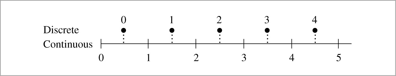
The second issue is that the pixels in the final image are naturally defined at discrete integer (x, y) coordinates on a pixel grid, but the Samplers in this chapter generate image samples at continuous floating-point (x, y) positions. The natural way to map between these two domains is to round continuous coordinates to the nearest discrete coordinate; this is appealing since it maps continuous coordinates that happen to have the same value as discrete coordinates to that discrete coordinate. However, the result is that given a set of discrete coordinates spanning a range [x0, x1], the set of continuous coordinates that covers that range is [x0 − 1/2, x1 + 1/2). Thus, any code that generates continuous sample positions for a given discrete pixel range is littered with 1/2 offsets. It is easy to forget some of these, leading to subtle errors.
If we instead truncate continuous coordinates c to discrete coordinates d by

and convert from discrete to continuous by

then the range of continuous coordinates for the discrete range [x0, x1] is naturally [x0, x1 + 1) and the resulting code is much simpler (Heckbert 1990a). This convention, which we will adopt in pbrt, is shown graphically in Figure 7.12.
7.2 Sampling interface
As first introduced in Section 7.1.5, the rendering approach implemented in pbrt involves choosing sample points in additional dimensions beyond 2D points on the image plane. Various algorithms will be used to generate these points, but all of their implementations inherit from an abstract Sampler class that defines their interface. The core sampling declarations and functions are in the files core/sampler.h and core/sampler.cpp. Each of the sample generation implementations is in its own source files in the samplers/directory.
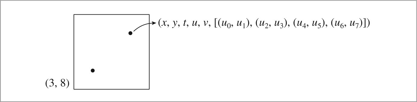
The task of a Sampler is to generate a sequence of n-dimensional samples in [0, 1)n, where one such sample vector is generated for each image sample and where the number of dimensions n in each sample may vary, depending on the calculations performed by the light transport algorithms. (See Figure 7.13.)
Because sample values must be strictly less than 1, it’s useful to define a constant, OneMinusEpsilon, that represents the largest representable floating-point constant that is less than 1. Later, we will clamp sample vector values to be no larger than this value.
〈Random Number Declarations〉 ≡
#ifdef PBRT_FLOAT_IS_DOUBLE
static const Float OneMinusEpsilon = 0x1.fffffffffffffp-1;
#else
static const Float OneMinusEpsilon = 0x1.fffffep-1;
#endif
The simplest possible implementation of a Sampler would just return uniform random values in [0, 1) each time an additional component of the sample vector was needed. Such a sampler would produce correct images but would require many more samples (and thus, many more rays traced and much more time) to create images of the same quality achievable with more sophisticated samplers. The run-time expense for using better sampling patterns is approximately the same as that for lower-quality patterns like uniform random numbers; because evaluating the radiance for each image sample is much more expensive than computing the sample’s component values, doing this work pays dividends (Figure 7.14).
A few characteristics of these sample vectors are assumed in the following:
• The first five dimensions generated by Samplers are generally used by the Camera. In this case, the first two are specifically used to choose a point on the image inside the current pixel area; the third is used to compute the time at which the sample should be taken; and the fourth and fifth dimensions give a (u, v) lens position for depth of field.
• Some sampling algorithms generate better samples in some dimensions of the sample vector than in others. Elsewhere in the system, we assume that in general, the earlier dimensions have the most well-placed sample values.
Note also that the n-dimensional samples generated by the Sampler are generally not represented explicitly or stored in their entirety but are often generated incrementally as needed by the light transport algorithm. (However, storing the entire sample vector and making incremental changes to its components is the basis of the MLTSampler in Section 16.4.4, which is used by the MLTIntegrator in Section 16.4.5.)
 7.2.1 Evaluating sample patterns: discrepancy
Fourier analysis gave us one way of evaluating the quality of a 2D sampling pattern, but it took us only as far as being able to quantify the improvement from adding more evenly spaced samples in terms of the band-limited frequencies that could be represented. Given the presence of infinite frequency content from edges in images and given the need for (n > 2)-dimensional sample vectors for Monte Carlo light transport algorithms, Fourier analysis alone isn’t enough for our needs.
Given a renderer and a candidate algorithm for placing samples, one way to evaluate the algorithm’s effectiveness is to use that sampling pattern to render an image and to compute the error in the image compared to a reference image rendered with a large number of samples. We will use this approach to compare sampling algorithms later in this chapter, though it only tells us how well the algorithm did for one specific scene, and it doesn’t give us a sense of the quality of the sample points without going through the rendering process.
Outside of Fourier analysis, mathematicians have developed a concept called discrepancy that can be used to evaluate the quality of a pattern of n-dimensional sample positions. Patterns that are well distributed (in a manner to be formalized shortly) have low discrepancy values, and thus the sample pattern generation problem can be considered to be one of finding a suitable low-discrepancy pattern of points.5 A number of deterministic techniques have been developed that generate low-discrepancy point sets, even in high-dimensional spaces. (Most of the sampling algorithms used later in this chapter use these techniques.)
The basic idea of discrepancy is that the quality of a set of points in an n-dimensional space [0, 1)n can be evaluated by looking at regions of the domain [0, 1)n, counting the number of points inside each region, and comparing the volume of each region to the number of sample points inside. In general, a given fraction of the volume should have roughly the same fraction of the total number of sample points inside of it. While it’s not possible for this always to be the case, we can still try to use patterns that minimize the maximum difference between the actual volume and the volume estimated by the points (the discrepancy). Figure 7.15 shows an example of the idea in two dimensions.

To compute the discrepancy of a set of points, we first pick a family of shapes B that are subsets of [0, 1)n. For example, boxes with one corner at the origin are often used. This corresponds to

where 0 ≤ vi < 1. Given a sequence of sample points P = x1, …, xN, the discrepancy of P with respect to B is6
where  {xi ∈ b} is the number of points in b and V (b) is the volume of b.
The intuition for why Equation (7.4) is a reasonable measure of quality is that the value {xi ∈ b}/N is an approximation of the volume of the box b given by the particular points P. Therefore, the discrepancy is the worst error over all possible boxes from this way of approximating volume. When the set of shapes B is the set of boxes with a corner at the origin, this value is called the star discrepancy, DN* (P). Another popular option for B is the set of all axis-aligned boxes, where the restriction that one corner be at the origin has been removed.
For a few particular point sets, the discrepancy can be computed analytically. For example, consider the set of points in one dimension

We can see that the star discrepancy of xi is
For example, take the interval b = [0, 1/N). Then V (b) = 1/N, but {xi ∈ b} = 0. This interval (and the intervals [0, 2/N), etc.) is the interval where the largest differences between volume and fraction of points inside the volume are seen.
The star discrepancy of this sequence can be improved by modifying it slightly:

Then

The bounds for the star discrepancy of a sequence of points in one dimension have been shown to be
Thus, the earlier sequence from Equation (7.5) has the lowest possible discrepancy for a sequence in 1D. In general, it is much easier to analyze and compute bounds for the discrepancy of sequences in 1D than for those in higher dimensions. For less simply constructed point sequences and for sequences in higher dimensions and for more irregular shapes than boxes, the discrepancy often must be estimated numerically by constructing a large number of shapes b, computing their discrepancy, and reporting the maximum value found.
The astute reader will notice that according to the low-discrepancy measure, this uniform sequence in 1D is optimal, but earlier in this chapter we claimed that irregular jittered patterns were perceptually superior to uniform patterns for image sampling in 2D since they replaced aliasing error with noise. In that framework, uniform samples are clearly not optimal. Fortunately, low-discrepancy patterns in higher dimensions are much less uniform than they are in one dimension and thus usually work reasonably well as sample patterns in practice. Nevertheless, their underlying uniformity means that low-discrepancy patterns can be more prone to visually objectionable aliasing than patterns with pseudo-random variation.
Discrepancy alone isn’t necessarily a good metric: some low-discrepancy point sets exhibit some clumping of samples, where two or more samples may be quite close together. The Sobol′ sampler in Section 7.7 particularly suffers from this issue—see Figure 7.36, which shows a plot of its first two dimensions. Intuitively, samples that are too close together aren’t a good use of sampling resources: the closer one sample is to another, the less likely it is to give useful new information about the function being sampled. Therefore, computing the minimum distance between any two samples in a set of points has also proved to be a useful metric of sample pattern quality; the higher the minimum distance, the better.
There are a variety of algorithms for generating Poisson disk sampling patterns that score well by this metric. By construction, no two points in a Poisson disk pattern are closer than some distance d. Studies have shown that the rods and cones in the eye are distributed in a similar way, which further validates the idea that this distribution is a good one for imaging. In practice, we have found that Poisson disk patterns work very well for sampling 2D images but are less effective than the better low discrepancy patterns for the higher-dimensional sampling done in more complex rendering situations; see the “Further Reading” section for more information.
7.2.2 Basic sampler interface
The Sampler base class not only defines the interface to samplers but also provides some common functionality for use by Sampler implementations.
〈Sampler Declarations〉 ≡
class Sampler {
public:
〈Sampler Interface 422〉
〈Sampler Public Data 422〉
protected:
〈Sampler Protected Data 425〉
private:
〈Sampler Private Data 426〉
};
All Sampler implementations must supply the constructor with the number of samples that will be generated for each pixel in the final image. In rare cases, it may be useful for the system to model the film as having only a single “pixel” that covers the entire viewing region. (This overloading of the definition of pixel is something of a stretch, but we allow it to simplify certain implementation aspects.) Since this “pixel” could potentially have billions of samples, we store the sample count using a variable with 64 bits of precision.
〈Sampler Method Definitions〉 ≡
Sampler::Sampler(int64_t samplesPerPixel)
: samplesPerPixel(samplesPerPixel) { }
〈Sampler Public Data〉 ≡ 421
const int64_t samplesPerPixel;
When the rendering algorithm is ready to start work on a given pixel, it starts by calling StartPixel(), providing the coordinates of the pixel in the image. Some Sampler implementations use the knowledge of which pixel is being sampled to improve the overall distribution of the samples that they generate for the pixel, while others ignore this information.
〈Sampler Interface〉 ≡ 421
virtual void StartPixel(const Point2i &p);
The Get1D() method returns the sample value for the next dimension of the current sample vector, and Get2D() returns the sample values for the next two dimensions. While a 2D sample value could be constructed by using values returned by a pair of calls to Get1D(), some samplers can generate better point distributions if they know that two dimensions will be used together.
〈Sampler Interface〉 + ≡ 421
virtual Float Get1D() = 0;
virtual Point2f Get2D() = 0;
In pbrt, we don’t support requests for 3D or higher dimensional sample values from samplers because these are generally not needed for the types of rendering algorithms implemented here. If necessary, multiple values from lower dimensional components can be used to construct higher dimensional sample points.
A sharp edge of these interfaces is that code that uses sample values must be carefully written so that it always requests sample dimensions in the same order. Consider the following code:
sampler- > StartPixel(p);
do {
Float v = a(sampler- > Get1D());
if (v > 0)
v + = b(sampler- > Get1D());
v + = c(sampler- > Get1D());
} while (sampler- > StartNextSample());
In this case, the first dimension of the sample vector will always be passed to the function a(); when the code path that calls b() is executed, b() will receive the second dimension. However, if the if test isn’t always true or false, then c() will sometimes receive a sample from the second dimension of the sample vector and otherwise receive a sample from the third dimension. Thus, efforts by the sampler to provide well-distributed sample points in each dimension being evaluated have been thwarted. Code that uses Samplers should therefore be carefully written so that it consistently consumes sample vector dimensions to avoid this issue.
For convenience, the Sampler base class provides a method that initializes a CameraSample for a given pixel.
〈Sampler Method Definitions〉 + ≡
CameraSample Sampler::GetCameraSample(const Point2i &pRaster) {
CameraSample cs;
cs.pFilm = (Point2f)pRaster + Get2D();
cs.time = Get1D();
cs.pLens = Get2D();
return cs;
}
Some rendering algorithms make use of arrays of sample values for some of the dimensions they sample; most sample-generation algorithms can generate higher quality arrays of samples than series of individual samples by accounting for the distribution of sample values across all elements of the array and across the samples in a pixel.
If arrays of samples are needed, they must be requested before rendering begins. The Request[12]DArray() methods should be called for each such dimension’s array before rendering begins—for example, in methods that override the SamplerIntegrator::Preprocess() method. For example, in a scene with two area light sources, where the integrator traces four shadow rays to the first source and eight to the second, the integrator would ask for two 2D sample arrays for each image sample, with four and eight samples each. (A 2D array is required because two dimensions are needed to parameterize the surface of a light.) In Section 13.7, we will see how using arrays of samples corresponds to more densely sampling some of the dimensions of the light transport integral using the Monte Carlo technique of “splitting.”
〈Sampler Interface〉 + ≡ 421
void Request1DArray(int n);
void Request2DArray(int n);
Most Samplers can do a better job of generating some particular sizes of these arrays than others. For example, samples from the ZeroTwoSequenceSampler are much better distributed in quantities that are in powers of 2. The Sampler::RoundCount() method helps communicate this information. Code that needs arrays of samples should call this method with the desired number of samples to be taken, giving the Sampler an opportunity to adjust the number of samples to a better number. The returned value should then be used as the number of samples to actually request from the Sampler. The default implementation returns the given count unchanged.
〈Sampler Interface〉 + ≡ 421
virtual int RoundCount(int n) const {
return n;
}
During rendering, the Get[12]DArray() methods can be called to get a pointer to the start of a previously requested array of samples for the current dimension. Along the lines of Get1D() and Get2D(), these return a pointer to an array of samples whose size is given by the parameter n to the corresponding call to Request[12]DArray() during initialization. The caller must also provide the array size to the “get” method, which is used to verify that the returned buffer has the expected size.
〈Sampler Interface〉 + ≡ 421
const Float *Get1DArray(int n);
const Point2f *Get2DArray(int n);
When the work for one sample is complete, the integrator calls StartNextSample(). This call notifies the Sampler that subsequent requests for sample components should return values starting at the first dimension of the next sample for the current pixel. This method returns true until the number of the originally requested samples per pixel have been generated (at which point the caller should either start work on another pixel or stop trying to use more samples.)
〈Sampler Interface〉 + ≡ 421
virtual bool StartNextSample();
Sampler implementations store a variety of state about the current sample: which pixel is being sampled, how many dimensions of the sample have been used, and so forth. It is therefore natural for it to be unsafe for a single Sampler to be used concurrently by multiple threads. The Clone() method generates a new instance of an initial Sampler for use by a rendering thread; it takes a seed value for the sampler’s random number generator (if any), so that different threads see different sequences of random numbers. Reusing the same pseudo-random number sequence across multiple image tiles can lead to subtle image artifacts, such as repeating noise patterns.
Implementations of the various Clone() methods aren’t generally interesting, so they won’t be included in the text here.
〈Sampler Interface〉 + ≡ 421
virtual std::unique_ptr < Sampler > Clone(int seed) = 0;
Some light transport algorithms (notably stochastic progressive photon mapping in Section 16.2) don’t use all of the samples in a pixel before going to the next pixel, but instead jump around pixels, taking one sample at a time in each one. The SetSampleNumber() method allows integrators to set the index of the sample in the current pixel to generate next. This method returns false once sampleNum is greater than or equal to the number of originally requested samples per pixel.
〈Sampler Interface〉 + ≡
virtual bool SetSampleNumber(int64_t sampleNum);
7.2.3 Sampler implementation
The Sampler base class provides implementations of some of the methods in its interface. First, the StartPixel() method implementation records the coordinates of the current pixel being sampled and resets currentPixelSampleIndex, the sample number in the pixel currently being generated, to zero. Note that this is a virtual method with an implementation; subclasses that override this method are required to explicitly call Sampler::StartPixel().
〈Sampler Method Definitions〉 + ≡
void Sampler::StartPixel(const Point2i &p) {
currentPixel = p;
currentPixelSampleIndex = 0;
〈Reset array offsets for next pixel sample 426〉
}
The current pixel coordinates and sample number within the pixel are made available to Sampler subclasses, though they should treat these as read-only values.
〈Sampler Protected Data〉 ≡ 421
Point2i currentPixel;
int64_t currentPixelSampleIndex;
When the pixel sample is advanced or explicitly set, currentPixelSampleIndex is updated accordingly. As with StartPixel(), the methods StartNextSample() and SetSampleNumber() are both virtual implementations; these implementations also must be explicitly called by overridden implementations of them in Sampler subclasses.
〈Sampler Method Definitions〉 + ≡
bool Sampler::StartNextSample() {
〈Reset array offsets for next pixel sample 426〉
return ++currentPixelSampleIndex < samplesPerPixel;
}
〈Sampler Method Definitions〉 + ≡
bool Sampler::SetSampleNumber(int64_t sampleNum) {
〈Reset array offsets for next pixel sample 426〉
currentPixelSampleIndex = sampleNum;
return currentPixelSampleIndex < samplesPerPixel;
}
The base Sampler implementation also takes care of recording requests for arrays of sample components and allocating storage for their values. The sizes of the requested sample arrays are stored in samples1DArraySizes and samples2DArraySizes, and memory for an entire pixel’s worth of array samples is allocated in sampleArray1D and sampleArray2D. The first n values in each allocation are used for the corresponding array for the first sample in the pixel, and so forth.
〈Sampler Method Definitions〉 + ≡
void Sampler::Request1DArray(int n) {
samples1DArraySizes.push_back(n);
sampleArray1D.push_back(std::vector < Float > (n * samplesPerPixel));
}
〈Sampler Method Definitions〉 + ≡
void Sampler::Request2DArray(int n) {
samples2DArraySizes.push_back(n);
sampleArray2D.push_back(std::vector < Point2f > (n * samplesPerPixel));
}
〈Sampler Protected Data〉 + ≡ 421
std::vector < int > samples1DArraySizes, samples2DArraySizes;
std::vector < std::vector < Float > > sampleArray1D;
std::vector < std::vector < Point2f > > sampleArray2D;
As arrays in the current sample are accessed by the Get[12]DArray() methods, array1D Offset and array2DOffset are updated to hold the index of the next array to return for the sample vector.
〈Sampler Private Data〉 ≡ 421
size_t array1DOffset, array2DOffset;
When a new pixel is started or when the sample number in the current pixel changes, these array offsets must be reset to 0.
〈Reset array offsets for next pixel sample〉 ≡ 425
array1DOffset = array2DOffset = 0;
Returning the appropriate array pointer is a matter of first choosing the appropriate array based on how many have been consumed in the current sample vector and then returning the appropriate instance of it based on the current pixel sample index.
〈Sampler Method Definitions〉 + ≡
const Float *Sampler::Get1DArray(int n) {
if (array1DOffset == sampleArray1D.size())
return nullptr;
return &sampleArray1D[array1DOffset++][currentPixelSampleIndex * n];
}
〈Sampler Method Definitions〉 + ≡
const Point2f *Sampler::Get2DArray(int n) {
if (array2DOffset == sampleArray2D.size())
return nullptr;
return &sampleArray2D[array2DOffset++][currentPixelSampleIndex * n];
}
7.2.4 Pixel sampler
While some sampling algorithms can easily incrementally generate elements of each sample vector, others more naturally generate all of the dimensions’ sample values for all of the sample vectors for a pixel at the same time. The PixelSampler class implements some functionality that is useful for the implementation of these types of samplers.
〈Sampler Declarations〉 + ≡
class PixelSampler : public Sampler {
public:
〈PixelSampler Public Methods〉
protected:
〈PixelSampler Protected Data 427〉
};
The number of dimensions of the sample vectors that will be used by the rendering algorithm isn’t known ahead of time. (Indeed, it’s only determined implicitly by the number of Get1D() and Get2D() calls and the requested arrays.) Therefore, the PixelSampler constructor takes a maximum number of dimensions for which non-array sample values will be computed by the Sampler. If all of these dimensions of components are consumed, then the PixelSampler just returns uniform random values for additional dimensions.
For each precomputed dimension, the constructor allocates a vector to store sample values, with one value for each sample in the pixel. These vectors are indexed as sample1D[dim][pixelSample]; while interchanging the order of these indices might seem more sensible, this memory layout—where all of the sample component values for all of the samples for a given dimension are contiguous in memory—turns out to be more convenient for code that generates these values.
〈Sampler Method Definitions〉 + ≡
PixelSampler::PixelSampler(int64_t samplesPerPixel,
int nSampledDimensions)
: Sampler(samplesPerPixel) {
for (int i = 0; i < nSampledDimensions; ++i) {
samples1D.push_back(std::vector < Float > (samplesPerPixel));
samples2D.push_back(std::vector < Point2f > (samplesPerPixel));
}
}
The key responsibility of Sampler implementations that inherit from PixelSampler then is to fill in the samples1D and samples2D arrays (in addition to sampleArray1D and sampleArray2D) in their StartPixel() methods.
current1DDimension and current2DDimension store the offsets into the respective arrays for the current pixel sample. They must be reset to 0 at the start of each new sample.
〈PixelSampler Protected Data〉 ≡ 427
std::vector < std::vector < Float > > samples1D;
std::vector < std::vector < Point2f > > samples2D;
int current1DDimension = 0, current2DDimension = 0;
〈Sampler Method Definitions〉 + ≡
bool PixelSampler::StartNextSample() {
current1DDimension = current2DDimension = 0;
return Sampler::StartNextSample();
}
〈Sampler Method Definitions〉 + ≡
bool PixelSampler::SetSampleNumber(int64_t sampleNum) {
current1DDimension = current2DDimension = 0;
return Sampler::SetSampleNumber(sampleNum);
}
Given sample values in the arrays computed by the PixelSampler subclass, the implementation of Get1D() is just a matter of returning values for successive dimensions until all of the computed dimensions have been consumed, at which point uniform random values are returned.
〈Sampler Method Definitions〉 + ≡
Float PixelSampler::Get1D() {
if (current1DDimension < samples1D.size())
return samples1D[current1DDimension++][currentPixelSampleIndex];
else
return rng.UniformFloat();
}
The PixelSampler::Get2D() follows similarly, so it won’t be included here.
The random number generator used by the PixelSampler is protected rather than private; this is a convenience for some of its subclasses that also need random numbers when they initialize samples1D and samples2D.
〈PixelSampler Protected Data〉 + ≡ 427
RNG rng;
7.2.5 Global sampler
Other algorithms for generating samples are very much not pixel-based but naturally generate consecutive samples that are spread across the entire image, visiting completely different pixels in succession. (Many such samplers are effectively placing each additional sample such that it fills the biggest hole in the n-dimensional sample space, which naturally leads to subsequent samples being inside different pixels.) These sampling algorithms are somewhat problematic with the Sampler interface as described so far: consider, for example, a sampler that generates the series of sample values shown in the middle column of Table 7.2 for the first two dimensions. These sample values are multiplied by the image resolution in each dimension to get sample positions in the image plane (here we’re considering a 2 × 3 image for simplicity.) Note that for the sampler here (actually the HaltonSampler), each pixel is visited by each sixth sample. If we are rendering an image with three samples per pixel, then to generate all of the samples for the pixel (0, 0), we need to generate the samples with indices 0, 6, and 12, and so forth.
Table 7.2
The HaltonSampler generates the coordinates in the middle column for the first two dimensions. Because it is a GlobalSampler, it must define an inverse mapping from the pixel coordinates to sample indices; here, it places samples across a 2 × 3 pixel image, by scaling the first coordinate by 2 and the second coordinate by three, giving the pixel sample coordinates in the right column.
| Sample index | [0, 1)2 sample coordinates | Pixel sample coordinates |
| 0 | (0.000000, 0.000000) | (0.000000, 0.000000) |
| 1 | (0.500000, 0.333333) | (1.000000, 1.000000) |
| 2 | (0.250000, 0.666667) | (0.500000, 2.000000) |
| 3 | (0.750000, 0.111111) | (1.500000, 0.333333) |
| 4 | (0.125000, 0.444444) | (0.250000, 1.333333) |
| 5 | (0.625000, 0.777778) | (1.250000, 2.333333) |
| 6 | (0.375000, 0.222222) | (0.750000, 0.666667) |
| 7 | (0.875000, 0.555556) | (1.750000, 1.666667) |
| 8 | (0.062500, 0.888889) | (0.125000, 2.666667) |
| 9 | (0.562500, 0.037037) | (1.125000, 0.111111) |
| 10 | (0.312500, 0.370370) | (0.625000, 1.111111) |
| 11 | (0.812500, 0.703704) | (1.625000, 2.111111) |
| 12 | (0.187500, 0.148148) | (0.375000, 0.444444) |
 |
Given the existence of such samplers, we could have defined the Sampler interface so that it specifies the pixel being rendered for each sample rather than the other way around (i.e., the Sampler being told which pixel to render).
However, there were good reasons to adopt the current design: this approach makes it easy to decompose the film into small image tiles for multi-threaded rendering, where each thread computes pixels in a local region that can be efficiently merged into the final image. Thus, we must require that such samplers generate samples out of order, so that all samples for each pixel are generated in succession.
The GlobalSampler helps bridge between the expectations of the Sampler interface and the natural operation of these types of samplers. It provides implementations of all of the pure virtual Sampler methods, implementing them in terms of three new pure virtual methods that its subclasses must implement instead.
〈Sampler Declarations〉 + ≡
class GlobalSampler : public Sampler {
public:
〈GlobalSampler Public Methods 429〉
private:
〈GlobalSampler Private Data 430〉
};
〈GlobalSampler Public Methods〉 ≡ 429
GlobalSampler(int64_t samplesPerPixel) : Sampler(samplesPerPixel) { }
There are two methods that implementations must provide. The first one, GetIndexFor Sample(), performs the inverse mapping from the current pixel and given sample index to a global index into the overall set of sample vectors. For example, for the Sampler that generated the values in Table 7.2, if currentPixel was (0, 2), then GetIndexForSample(0) would return 2, since the corresponding pixel sample coordinates for sample index 2, (0.25, 0.666667) correspond to the first sample that lands in that pixel’s area.
〈GlobalSampler Public Methods〉 + ≡ 429
virtual int64_t GetIndexForSample(int64_t sampleNum) const = 0;
Closely related, SampleDimension() returns the sample value for the given dimension of the index th sample vector in the sequence. Because the first two dimensions are used to offset into the current pixel, they are handled specially: the value returned by implementations of this method should be the sample offset within the current pixel, rather than the original [0, 1)2 sample value. For the example in Table 7.2, SampleDimension(4,1) would return 0.333333, since the second dimension of the sample with index 4 is that offset into the pixel (0, 1).
〈GlobalSampler Public Methods〉 + ≡ 429
virtual Float SampleDimension(int64_t index, int dimension) const = 0;
When it’s time to start to generate samples for a pixel, it’s necessary to reset the dimension of the sample and find the index of the first sample in the pixel. As with all samplers, values for sample arrays are all generated next.
〈Sampler Method Definitions〉 + ≡
void GlobalSampler::StartPixel(const Point2i &p) {
Sampler::StartPixel(p);
dimension = 0;
intervalSampleIndex = GetIndexForSample(0);
〈Compute arrayEndDim for dimensions used for array samples 431〉
〈Compute 1D array samples for GlobalSampler 431〉
〈Compute 2D array samples for GlobalSampler〉
}
The dimension member variable tracks the next dimension that the sampler implementation will be asked to generate a sample value for; it’s incremented as Get1D() and Get2D() are called. intervalSampleIndex records the index of the sample that corresponds to the current sample si in the current pixel.
〈GlobalSampler Private Data〉 ≡ 429
int dimension;
int64_t intervalSampleIndex;
It’s necessary to decide which dimensions of the sample vector to use for array samples. Under the assumption that the earlier dimensions will be better quality than later dimensions, it’s important to set aside the first few dimensions for the CameraSample, since the quality of those sample values often has a large impact on final image quality.
Therefore, the first dimensions up to arrayStartDim are devoted to regular 1D and 2D samples, and then the subsequent dimensions are devoted to first 1D and then 2D array samples. Finally, higher dimensions starting at arrayEndDim are used for further non-array 1D and 2D samples. It isn’t possible to compute arrayEndDim when the GlobalSampler constructor runs, since array samples haven’t been requested yet by the integrators. Therefore, this value is computed (repeatedly and redundantly) in the StartPixel() method.
〈GlobalSampler Private Data〉 + ≡ 429
static const int arrayStartDim = 5;
int arrayEndDim;
The total number of array samples for all pixel samples is given by the product of the number of pixel samples and the requested sample array size.
〈Compute arrayEndDim for dimensions used for array samples〉 ≡ 430
arrayEndDim = arrayStartDim +
sampleArray1D.size() + 2 * sampleArray2D.size();
Actually generating the array samples is just a matter of computing the number of needed values in the current sample dimension.
〈Compute 1D array samples for GlobalSampler〉 ≡ 430
for (size_t i = 0; i < samples1DArraySizes.size(); ++i) {
int nSamples = samples1DArraySizes[i] * samplesPerPixel;
for (int j = 0; j < nSamples; ++j) {
int64_t index = GetIndexForSample(j);
sampleArray1D[i][j] =
SampleDimension(index, arrayStartDim + i);
}
}
The 2D sample arrays are generated analogously; the 〈Compute 2D array samples for GlobalSampler〉 fragment isn’t included here.
When the pixel sample changes, it’s necessary to reset the current sample dimension counter and to compute the sample index for the next sample inside the pixel.
〈Sampler Method Definitions〉 + ≡
bool GlobalSampler::StartNextSample() {
dimension = 0;
intervalSampleIndex = GetIndexForSample(currentPixelSampleIndex + 1);
return Sampler::StartNextSample();
}
〈Sampler Method Definitions〉 + ≡
bool GlobalSampler::SetSampleNumber(int64_t sampleNum) {
dimension = 0;
intervalSampleIndex = GetIndexForSample(sampleNum);
return Sampler::SetSampleNumber(sampleNum);
}
Given this machinery, getting regular 1D sample values is just a matter of skipping over the dimensions allocated to array samples and passing the current sample index and dimension to the implementation’s SampleDimension() method.
〈Sampler Method Definitions〉 + ≡
Float GlobalSampler::Get1D() {
if (dimension > = arrayStartDim && dimension < arrayEndDim)
dimension = arrayEndDim;
return SampleDimension(intervalSampleIndex, dimension++);
}
2D samples follow analogously.
〈Sampler Method Definitions〉 + ≡
Point2f GlobalSampler::Get2D() {
if (dimension + 1 > = arrayStartDim && dimension < arrayEndDim)
dimension = arrayEndDim;
Point2f p(SampleDimension(intervalSampleIndex, dimension),
SampleDimension(intervalSampleIndex, dimension + 1));
dimension + = 2;
return p;
}
7.3 Stratified sampling
The first Sampler implementation that we will introduce subdivides pixel areas into rectangular regions and generates a single sample inside each region. These regions are commonly called strata, and this sampler is called the StratifiedSampler. The key idea behind stratification is that by subdividing the sampling domain into nonoverlapping regions and taking a single sample from each one, we are less likely to miss important features of the image entirely, since the samples are guaranteed not to all be close together. Put another way, it does us no good if many samples are taken from nearby points in the sample space, since each new sample doesn’t add much new information about the behavior of the image function. From a signal processing viewpoint, we are implicitly defining an overall sampling rate such that the smaller the strata are, the more of them we have, and thus the higher the sampling rate.
The stratified sampler places each sample at a random point inside each stratum by jittering the center point of the stratum by a random amount up to half the stratum’s width and height. The nonuniformity that results from this jittering helps turn aliasing into noise, as discussed in Section 7.1. The sampler also offers an unjittered mode, which gives uniform sampling in the strata; this mode is mostly useful for comparisons between different sampling techniques rather than for rendering high quality images.
Direct application of stratification to high-dimensional sampling quickly leads to an intractable number of samples. For example, if we divided the 5D image, lens, and time sample space into four strata in each dimension, the total number of samples per pixel would be 45 = 1024. We could reduce this impact by taking fewer samples in some dimensions (or not stratifying some dimensions, effectively using a single stratum), but we would then lose the benefit of having well-stratified samples in those dimensions. This problem with stratification is known as the curse of dimensionality.
We can reap most of the benefits of stratification without paying the price in excessive total sampling by computing lower dimensional stratified patterns for subsets of the domain’s dimensions and then randomly associating samples from each set of dimensions. (This process is sometimes called padding.) Figure 7.16 shows the basic idea: we might want to take just four samples per pixel but still have the samples be stratified over all dimensions. We independently generate four 2D stratified image samples, four 1D stratified time samples, and four 2D stratified lens samples. Then we randomly associate a time and lens sample value with each image sample. The result is that each pixel has samples that together have good coverage of the sample space. Figure 7.17 shows the improvement in image quality from using stratified lens samples versus using unstratified random samples when rendering depth of field.

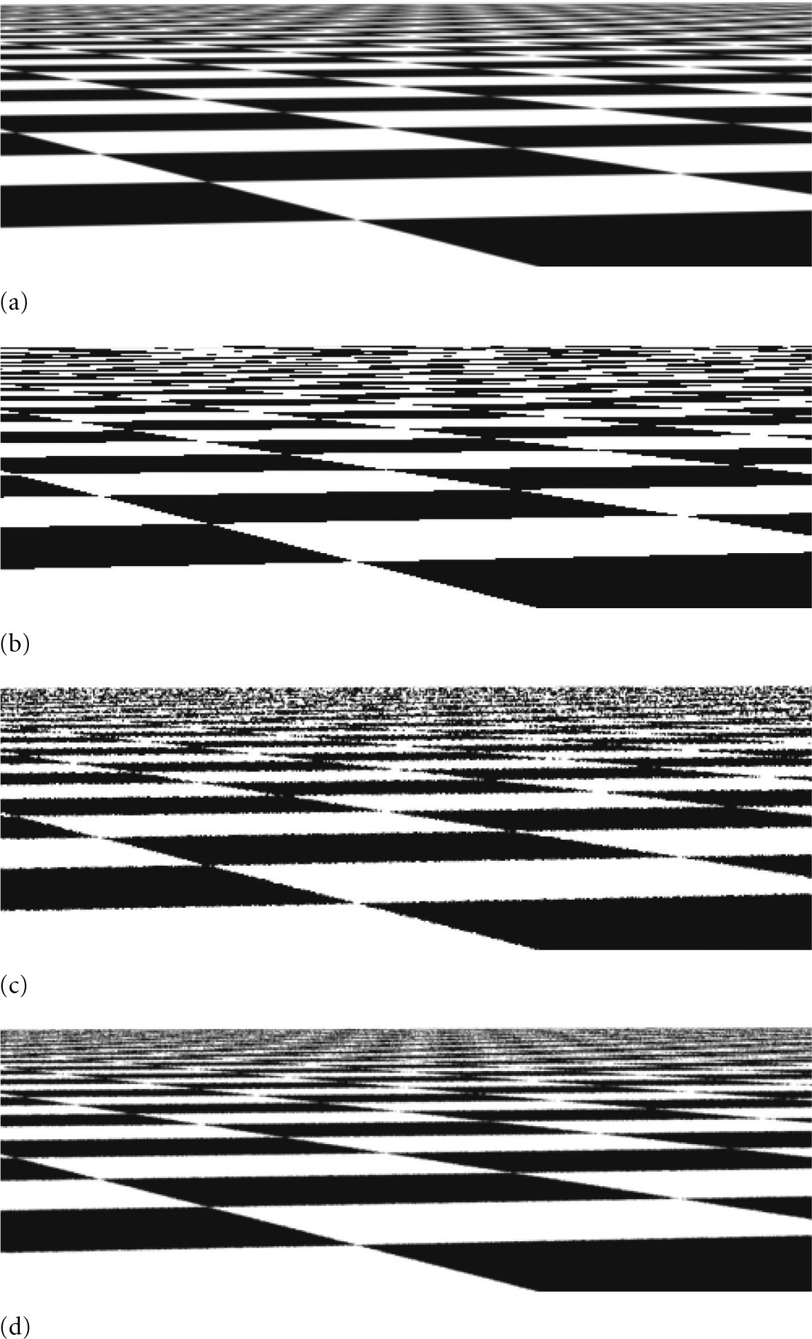
Figure 7.18 shows a comparison of a few sampling patterns. The first is a completely random pattern: we generated a number of samples without using the strata at all. The result is terrible; some regions have few samples and other areas have clumps of many samples. The second is a uniform stratified pattern. In the last, the uniform pattern has been jittered, with a random offset added to each sample’s location, keeping it inside its cell. This gives a better overall distribution than the purely random pattern while preserving the benefits of stratification, though there are still some clumps of samples and some regions that are undersampled. Figure 7.19 shows images rendered using the StratifiedSampler and shows how jittered sample positions turn aliasing artifacts into less objectionable noise.

〈StratifiedSampler Declarations〉 ≡
class StratifiedSampler : public PixelSampler {
public:
〈StratifiedSampler Public Methods 434〉
private:
〈StratifiedSampler Private Data 434〉
};
〈StratifiedSampler Public Methods〉 ≡ 434
StratifiedSampler(int xPixelSamples, int yPixelSamples,
bool jitterSamples, int nSampledDimensions)
: PixelSampler(xPixelSamples * yPixelSamples, nSampledDimensions),
xPixelSamples(xPixelSamples), yPixelSamples(yPixelSamples),
jitterSamples(jitterSamples) { }
〈StratifiedSampler Private Data〉 ≡ 434
const int xPixelSamples, yPixelSamples;
const bool jitterSamples;
As a PixelSampler subclass, the implementation of StartPixel() must both generate 1D and 2D samples for the number of dimensions nSampledDimensions passed to the PixelSampler constructor as well as samples for the requested arrays.
〈StratifiedSampler Method Definitions〉 ≡
void StratifiedSampler::StartPixel(const Point2i &p) {
〈Generate single stratified samples for the pixel 437〉
〈Generate arrays of stratified samples for the pixel 440〉
PixelSampler::StartPixel(p);
}
After the initial stratified samples are generated, they are randomly shuffled; this is the padding approach described at the start of the section. If this shuffling wasn’t done, then the sample dimensions’ values would be correlated in a way that would lead to errors in images—for example, both the first 2D sample used to choose the film location as well as the first 2D lens sample would always both be in the lower left stratum adjacent to the origin.
〈Generate single stratified samples for the pixel〉 ≡ 434
for (size_t i = 0; i < samples1D.size(); ++i) {
StratifiedSample1D(&samples1D[i][0], xPixelSamples * yPixelSamples,
rng, jitterSamples);
Shuffle(&samples1D[i][0], xPixelSamples * yPixelSamples, 1, rng);
}
for (size_t i = 0; i < samples2D.size(); ++i) {
StratifiedSample2D(&samples2D[i][0], xPixelSamples, yPixelSamples,
rng, jitterSamples);
Shuffle(&samples2D[i][0], xPixelSamples * yPixelSamples, 1, rng);
}
The 1D and 2D stratified sampling routines are implemented as utility functions. Both loop over the given number of strata in the domain and place a sample point in each one.
〈Sampling Function Definitions〉 ≡
void StratifiedSample1D(Float *samp, int nSamples, RNG &rng,
bool jitter) {
Float invNSamples = (Float)1 / nSamples;
for (int i = 0; i < nSamples; ++i) {
Float delta = jitter ? rng.UniformFloat() : 0.5f;
samp[i] = std::min((i + delta) * invNSamples, OneMinusEpsilon);
}
}
StratifiedSample2D() similarly generates samples in the range [0, 1)2.
〈Sampling Function Definitions〉 + ≡
void StratifiedSample2D(Point2f *samp, int nx, int ny, RNG &rng,
bool jitter) {
Float dx = (Float)1 / nx, dy = (Float)1 / ny;
for (int y = 0; y < ny; ++y)
for (int x = 0; x < nx; ++x) {
Float jx = jitter ? rng.UniformFloat() : 0.5f;
Float jy = jitter ? rng.UniformFloat() : 0.5f;
samp- > x = std::min((x + jx) * dx, OneMinusEpsilon);
samp- > y = std::min((y + jy) * dy, OneMinusEpsilon);
++samp;
}
}
The Shuffle() function randomly permutes an array of count sample values, each of which has nDimensions dimensions. (In other words, blocks of values of size nDimensions are permuted.)
〈Sampling Inline Functions〉 ≡
template < typename T >
void Shuffle(T *samp, int count, int nDimensions, RNG &rng) {
for (int i = 0; i < count; ++i) {
int other = i + rng.UniformUInt32(count - i);
for (int j = 0; j < nDimensions; ++j)
std::swap(samp[nDimensions * i + j],
samp[nDimensions * other + j]);
}
}
Arrays of samples present us with a quandary: for example, if an integrator asks for an array of 64 2D sample values in the sample vector for each sample in a pixel, the sampler has two different goals to try to fulfill:
1. It’s desirable that the samples in the array themselves be well distributed in 2D (e.g., by using an 8 × 8 stratified grid). Stratification here will improve the quality of the computed results for each individual sample vector.
2. It’s desirable to ensure that each the samples in the array for one image sample isn’t too similar to any of the sample values for samples nearby in the image. Rather, we’d like the points to be well distributed with respect to their neighbors, so that over the region around a single pixel, there is good coverage of the entire sample space.
Rather than trying to solve both of these problems simultaneously here, the Stratified Sampler only addresses the first one. The other samplers later in this chapter will revisit this issue with more sophisticated techniques and solve both of them simultaneously to various degrees.
A second complication comes from the fact that the caller may have asked for an arbitrary number of samples per image sample, so stratification may not be easily applied. (For example, how do we generate a stratified 2D pattern of seven samples?) We could just generate an n × 1 or 1 × n stratified pattern, but this only gives us the benefit of stratification in one dimension and no guarantee of a good pattern in the other dimension. A StratifiedSampler::RoundSize() method could round requests up to the next number that’s the square of integers, but instead we will use an approach called Latin hypercube sampling (LHS), which can generate any number of samples in any number of dimensions with a reasonably good distribution.
LHS uniformly divides each dimension’s axis into n regions and generates a jittered sample in each of the n regions along the diagonal, as shown on the left in Figure 7.20. These samples are then randomly shuffled in each dimension, creating a pattern with good distribution. An advantage of LHS is that it minimizes clumping of the samples when they are projected onto any of the axes of the sampling dimensions. This property is in contrast to stratified sampling, where 2n of the n × n samples in a 2D pattern may project to essentially the same point on each of the axes. Figure 7.21 shows this worst-case situation for a stratified sampling pattern.

In spite of addressing the clumping problem, LHS isn’t necessarily an improvement to stratified sampling; it’s easy to construct cases where the sample positions are essentially colinear and large areas of the sampling domain have no samples near them (e.g., when the permutation of the original samples is the identity, leaving them all where they started). In particular, as n increases, Latin hypercube patterns are less and less effective compared to stratified patterns.7
The general-purpose LatinHypercube() function generates an arbitrary number of LHS samples in an arbitrary dimension. The number of elements in the samples array should thus be nSamples*nDim.
〈Sampling Function Definitions〉 + ≡
void LatinHypercube(Float *samples, int nSamples, int nDim, RNG &rng) {
〈Generate LHS samples along diagonal 440〉
〈Permute LHS samples in each dimension 440〉
}
〈Generate LHS samples along diagonal〉 ≡ 440
Float invNSamples = (Float)1 / nSamples;
for (int i = 0; i < nSamples; ++i)
for (int j = 0; j < nDim; ++j) {
Float sj = (i + (rng.UniformFloat())) * invNSamples;
samples[nDim * i + j] = std::min(sj, OneMinusEpsilon);
}
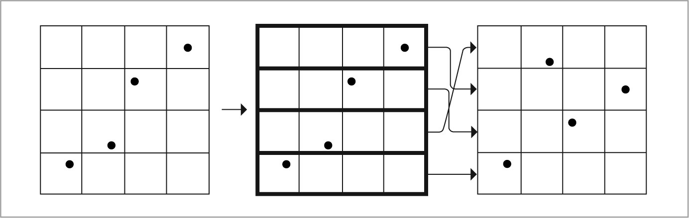
To do the permutation, this function loops over the samples, randomly permuting the sample points in one dimension at a time. Note that this is a different permutation than the earlier Shuffle() routine: that routine does one permutation, keeping all nDim sample points in each sample together, while here nDim separate permutations of a single dimension at a time are done (Figure 7.22).8

〈Permute LHS samples in each dimension〉 ≡ 440
for (int i = 0; i < nDim; ++i) {
for (int j = 0; j < nSamples; ++j) {
int other = j + rng.UniformUInt32(nSamples - j);
std::swap(samples[nDim * j + i], samples[nDim * other + i]);
}
}
Given the LatinHypercube() function, we can now write the code to compute sample arrays for the current pixel. 1D samples are stratified and then randomly shuffled, while 2D samples are generated using Latin hypercube sampling.
〈Generate arrays of stratified samples for the pixel〉 ≡ 434
for (size_t i = 0; i < samples1DArraySizes.size(); ++i)
for (int64_t j = 0; j < samplesPerPixel; ++j) {
int count = samples1DArraySizes[i];
StratifiedSample1D(&sampleArray1D[i][j * count], count, rng,
jitterSamples);
Shuffle(&sampleArray1D[i][j * count], count, 1, rng);
}
for (size_t i = 0; i < samples2DArraySizes.size(); ++i)
for (int64_t j = 0; j < samplesPerPixel; ++j) {
int count = samples2DArraySizes[i];
LatinHypercube(&sampleArray2D[i][j * count].x, count, 2, rng);
}
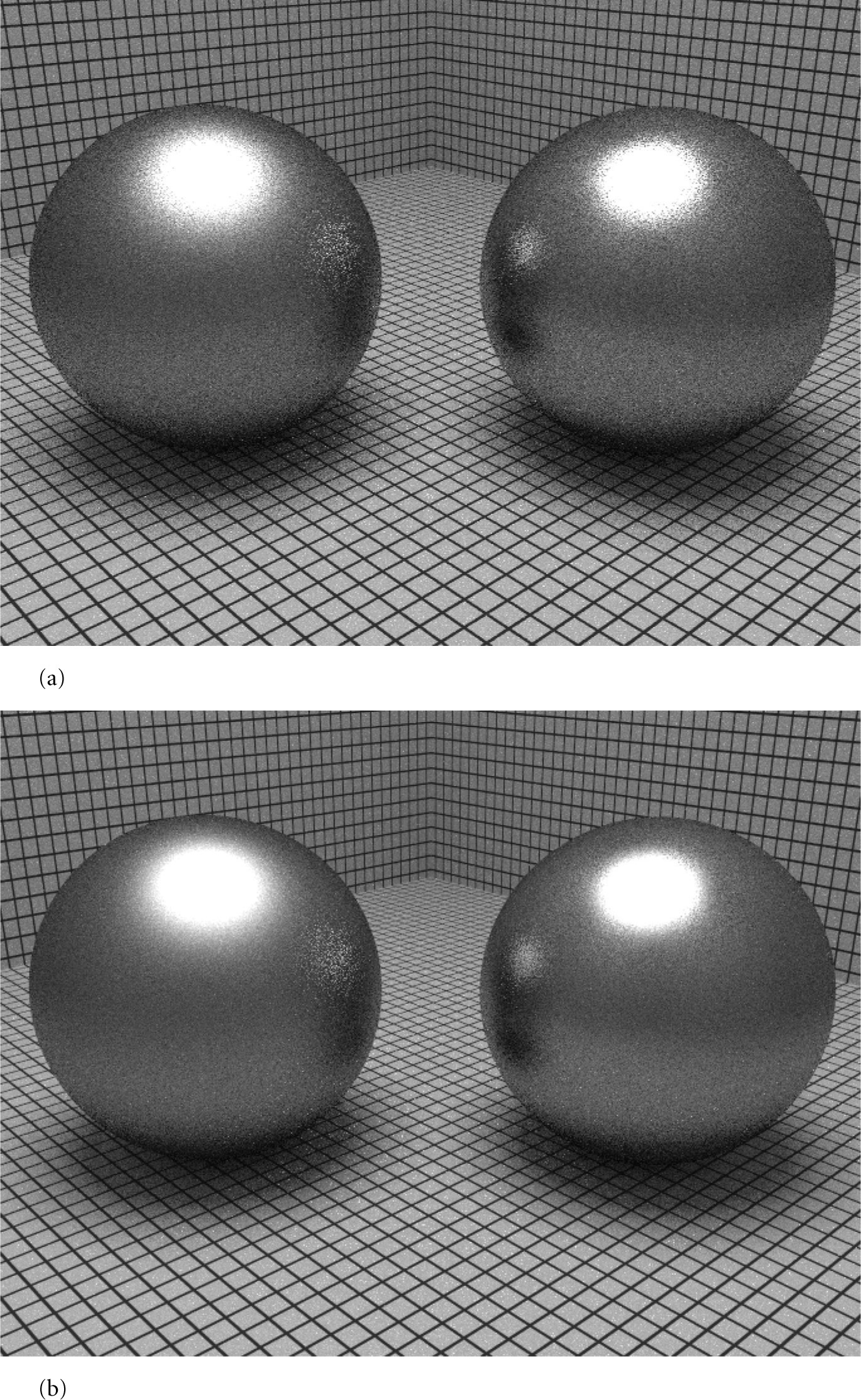
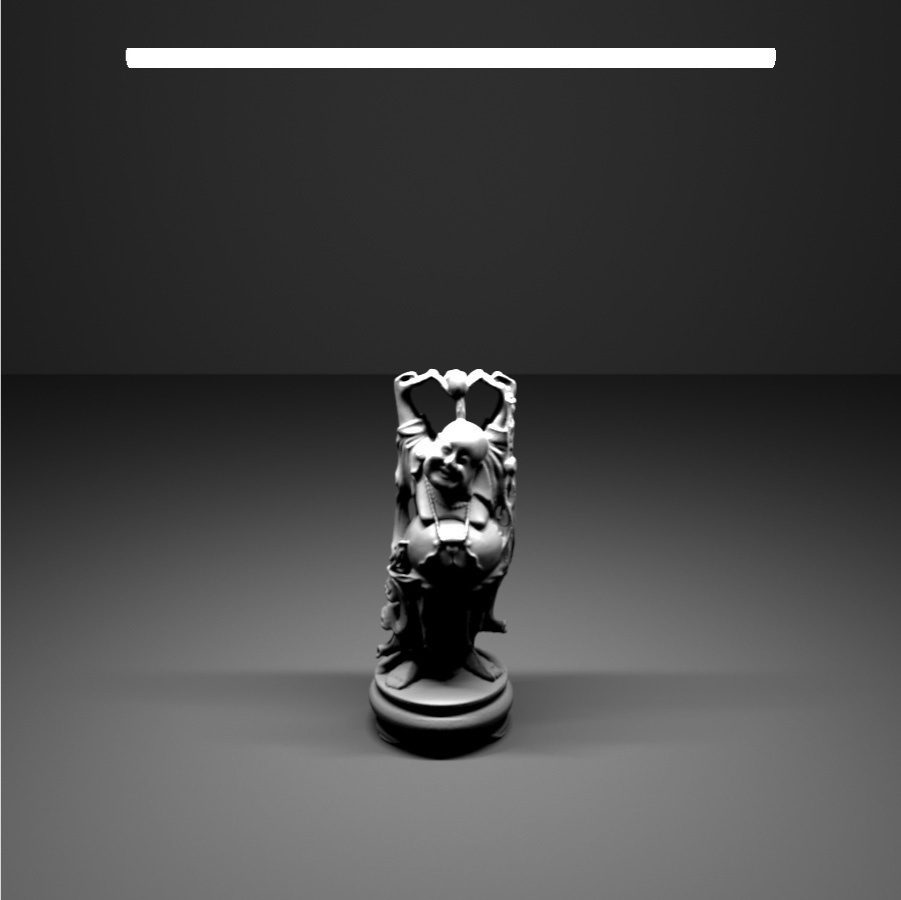
Starting with the scene in Figure 7.23, Figure 7.24 shows the improvement from good samples for the DirectLightingIntegrator. Image (a) was computed with 1 image sample per pixel, each with 16 shadow samples, and image (b) was computed with 16 image samples per pixel, each with 1 shadow sample. Because the StratifiedSampler could generate a good LHS pattern for the first case, the quality of the shadow is much better, even with the same total number of shadow samples taken.

* 7.4 The halton sampler
The underlying goal of the StratifiedSampler is to generate a well-distributed but non-uniform set of sample points, with no two sample points too close together and no excessively large regions of the sample space that have no samples. As Figure 7.18 showed, a jittered pattern does this much better than a random pattern does, although its quality can suffer when samples in adjacent strata happen to be close to the shared boundary of their two strata.
This section introduces the HaltonSampler, which is based on algorithms that directly generate low-discrepancy point sets. Unlike the points generated by the Stratified Sampler, the HaltonSampler not only generates points that are guaranteed to not clump too closely together, but it also generates points that are simultaneously well distributed over all of the dimensions of the sample vector—not just one or two dimensions at a time, as the StratifiedSampler did.
7.4.1 Hammersley and halton sequences
The Halton and Hammersley sequences are two closely related low-discrepancy point sets. Both are based on a construction called the radical inverse, which is based on the fact that a positive integer value a can be expressed in a base b with a sequence of digits dm(a) … d2(a)d1(a) uniquely determined by

where all digits di (a) are between 0 and b − 1.
The radical inverse function Φb in base b converts a nonnegative integer a to a fractional value in [0, 1) by reflecting these digits about the radix point:

Thus, the contribution of the digit di(a) to the radical inverse is di (a)/bi.
One of the simplest low-discrepancy sequences is the van der Corput sequence, which is a 1D sequence given by the radical inverse function in base 2:

Table 7.3 shows the first few values of the van der Corput sequence. Notice how it recursively splits the intervals of the 1D line in half, generating a sample point at the center of each interval. The discrepancy of this sequence is

Table 7.3
The radical inverse Φ2(a) of the first few non-negative integers, computed in base 2. Notice how successive values of Φ2(a) are not close to any of the previous values of Φ2(a). As more and more values of the sequence are generated, samples are necessarily closer to previous samples, although with a minimum distance that is guaranteed to be reasonably good.
| a | Base 2 | Φ2(a) |
| 0 | 0 | 0 |
| 1 | 1 | 0.1 = 1/2 |
| 2 | 10 | 0.01 = 1/4 |
| 3 | 11 | 0.11 = 3/4 |
| 4 | 100 | 0.001 = 1/8 |
| 5 | 101 | 0.101 = 5n8 |
|
which matches the best discrepancy that has been attained for infinite sequences in n dimensions,
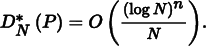
To generate points in an n-dimensional Halton sequence, we use the radical inverse base b, with a different base for each dimension of the pattern. The bases used must all be relatively prime to each other, so a natural choice is to use the first n prime numbers (p1, …, pn):

One of the most useful characteristics of the Halton sequence is that it can be used even if the total number of samples needed isn’t known in advance; all prefixes of the sequence are well distributed, so as additional samples are added to the sequence low discrepancy will be maintained. (However, its distribution is best when the total number of samples is the product of powers of the bases  for exponents ki.)
The discrepancy of an n-dimensional Halton sequence is

which is asymptotically optimal.
If the number of samples N is fixed, the Hammersley point set can be used, giving slightly lower discrepancy. Hammersley point sets are defined by

where N is the total number of samples to be taken and as before all of the bases bi are relatively prime. Figure 7.25(a) shows a plot of the first 216 points of the 2D Halton sequence. Figure 7.25(b) shows the first 256 points of the Hammersley sequence.
The function RadicalInverse() computes the radical inverse for a given number a using the baseIndex th prime number as the base. The function is implemented using an enormous switch statement, where baseIndex is mapped to the appropriate prime number and then a separate RadicalInverseSpecialized() template function actually computes the radical inverse. (The reason for the curious switch -based structure will be explained in a few pages.)
〈Low Discrepancy Function Definitions〉 ≡
Float RadicalInverse(int baseIndex, uint64_t a) {
switch (baseIndex) {
case 0:
〈Compute base-2 radical inverse 446〉
case 1: return RadicalInverseSpecialized < 3 > (a);
case 2: return RadicalInverseSpecialized < 5 > (a);
case 3: return RadicalInverseSpecialized < 7 > (a);
〈Remainder of cases for RadicalInverse()〉
}
}
For the base-2 radical inverse, we can take advantage of the fact that numbers in digital computers are already represented in base 2 to compute the radical inverse more efficiently. For a 64-bit value a, we have from Equation (7.6)

First consider the result of reversing the bits of a, still considering it as an integer value, which gives
If we then divide this value by 264, we have

which is Φ2(a). Thus, the base-2 radical inverse can equivalently be computed with a bit reverse and a power-of-two division.
The bits of an integer quantity can be efficiently reversed with a series of logical bit operations. The first line of the ReverseBits32() function, which reverses the bits of a 32-bit integer, swaps the lower 16 bits with the upper 16 bits of the value. The next line simultaneously swaps the first 8 bits of the result with the second 8 bits and the third 8 bits with the fourth. This process continues until the last line, which swaps adjacent bits.
To understand this code, it’s helpful to write out the binary values of the various hexadecimal constants. For example, 0xff00ff00 is 11111111000000001111111100000000 in binary; it’s easy to see that a bitwise OR with this value masks off the first and third 8-bit quantities.
〈Low Discrepancy Inline Functions〉 ≡
inline uint32_t ReverseBits32(uint32_t n) {
n = (n < < 16) | (n > > 16);
n = ((n & 0x00ff00ff) < < 8) | ((n & 0xff00ff00) > > 8);
n = ((n & 0x0f0f0f0f) < < 4) | ((n & 0xf0f0f0f0) > > 4);
n = ((n & 0x33333333) < < 2) | ((n & 0xcccccccc) > > 2);
n = ((n & 0x55555555) < < 1) | ((n & 0xaaaaaaaa) > > 1);
return n;
}
The bits of a 64-bit value can then be reversed by reversing the two 32-bit components individually and then interchanging them.
〈Low Discrepancy Inline Functions〉 + ≡
inline uint64_t ReverseBits64(uint64_t n) {
uint64_t n0 = ReverseBits32((uint32_t)n);
uint64_t n1 = ReverseBits32((uint32_t)(n > > 32));
return (n0 < < 32) | n1;
}
To compute the base-2 radical inverse, then, we reverse the bits and multiply by 1/264, where the hexadecimal floating-point constant 0x1p-64 is used for the value 2− 64. As explained in Section 3.9.1, implementing a power-of-two division via the corresponding power-of-two multiplication gives the same result with IEEE floating point. (And floating-point multiplication is generally more efficient than floating-point division.)
〈Compute base-2 radical inverse〉 ≡ 444
return ReverseBits64(a) * 0x1p-64;
For other bases, the RadicalInverseSpecialized() template function computes the radical inverse by computing the digits di starting with d1 and computing a series vi where v1 = d1, v2 = bd1 + d2 such that

(For example, in base 10, it would convert the value 1234 to 4321.) This value can be found entirely using integer arithmetic, without accumulating any round-off error.
The final value of the radical inverse is then found by converting to floating-point and multiplying by 1/bn, where n is the number of digits in the value, to get the value in Equation (7.7). The term for this multiplication is built up in invBaseN as the digits are processed.
〈Low Discrepancy Static Functions〉 ≡
template < int base >
static Float RadicalInverseSpecialized(uint64_t a) {
const Float invBase = (Float)1 / (Float)base;
uint64_t reversedDigits = 0;
Float invBaseN = 1;
while (a) {
uint64_t next = a / base;
uint64_t digit = a - next * base;
reversedDigits = reversedDigits * base + digit;
invBaseN * = invBase;
a = next;
}
return std::min(reversedDigits * invBaseN, OneMinusEpsilon);
}
A natural question to ask would be why a template function parameterized on the base is used here (rather than, say, a regular function call that took the base as a parameter, which would avoid the generation of a separate code path for each base). The motivation is that integer division is shockingly slow on modern CPUs, and much more efficient approaches are possible for division by a compile-time constant.
For example, integer division of a 32-bit value by 3 can be computed exactly by multiplying this value by 2863311531 to get a 64-bit intermediate and then shifting the result right by 33 bits; these are both fairly efficient operations. (A similar approach can be used for dividing 64-bit values by 3, but the magic constant is much larger; see Warren (2006) for more about these techniques.) Thus, using a template function here allows the compiler to see that the division to compute the value of next in the while loop is actually a division by a constant and gives it a chance to apply this optimization. The code with this optimization runs 5.9 times faster on a 2015-era laptop than an implementation based on integer division instructions.
Another optimization is that we avoid computing a running sum over reversed digits multiplied by the reciprocal base; instead, this multiplication is postponed all the way until the end when the loop terminates. The main issue here is that floating-point and integer units on current processors operate fairly independently from each other. Referencing an integer variable within a floating computation in a tight loop would introduce pipeline bubbles related to the amount of time that is needed to convert and move the values from one unit to the other.
It will be useful to be able to compute the inverse of the radical inverse function; the InverseRadicalInverse() function takes the reversed integer digits in some base, corresponding to value in the RadicalInverseSpecialized() template function immediately before being multiplied by the 1/bn factor to convert to a floating-point value in [0, 1). Note that in order to be able to compute the inverse correctly, the total number of digits in the original value must be known: for example, both 1234 and 123400 are converted to 4321 after the integer-only part of the radical inverse algorithm; trailing zeros become leading zeros, which are lost.
〈Low Discrepancy Inline Functions〉 + ≡
template < int base > inline uint64_t
InverseRadicalInverse(uint64_t inverse, int nDigits) {
uint64_t index = 0;
for (int i = 0; i < nDigits; ++i) {
uint64_t digit = inverse % base;
inverse /= base;
index = index * base + digit;
}
return index;
}
The Hammersley and Halton sequences have the shortcoming that as the base b increases, sample values can exhibit surprisingly regular patterns. This issue can be addressed with scrambled Halton and Hammersley sequences, where a permutation is applied to the digits when computing the radical inverse:

where p is a permutation of the digits (0, 1, … , b − 1). Note that the same permutation is used for each digit, and the same permutation is used for generating all of the sample points in a given base b. Figure 7.26 shows the effect of scrambling with the Halton sequence. In the following, we will use random permutations, though specific constructions of permutations can give slightly better results; see the “Further Reading” section for more details.
The ComputeRadicalInversePermutations() function computes these random permutation tables. It initializes a single contiguous array for all of the permutations, where the first two values are a permutation of the integers zero and one for b = 2, the next three values are a permutation of 0, 1, 2 for b = 3, and so forth for successive prime bases. At entry to the for loop below, p points to the start of the permutation array to initialize for the current prime base.
〈Low Discrepancy Function Definitions〉 + ≡
std::vector < uint16_t > ComputeRadicalInversePermutations(RNG &rng) {
std::vector < uint16_t > perms;
〈Allocate space in perms for radical inverse permutations 449〉
uint16_t *p = &perms[0];
for (int i = 0; i < PrimeTableSize; ++i) {
〈Generate random permutation for ith prime base 449〉
p + = Primes[i];
}
return perms;
}
The total size of the permutation array is given by the sum of the prime numbers up to the end of a precomputed table of prime numbers.
〈Allocate space in perms for radical inverse permutations〉 ≡ 449
int permArraySize = 0;
for (int i = 0; i < PrimeTableSize; ++i)
permArraySize + = Primes[i];
perms.resize(permArraySize);
〈Low Discrepancy Declarations〉 ≡
static constexpr int PrimeTableSize = 1000;
extern const int Primes[PrimeTableSize];
〈Low Discrepancy Data Definitions〉 ≡
const int Primes[PrimeTableSize] = {
2, 3, 5, 7, 11,
〈Subsequent prime numbers〉
};
Generating each permutation is easy: we just initialize p to the identity permutation for the current prime length and then randomly shuffle its values.
〈Generate random permutation for ith prime base〉 ≡ 449
for (int j = 0; j < Primes[i]; ++j)
p[j] = j;
Shuffle(p, Primes[i], 1, rng);
The ScrambledRadicalInverse() function is essentially the same as RadicalInverse() except that it puts each digit through the permutation table for the given base. See Exercise 7.1 for discussion of a more efficient implementation for the base-2 case, following RadicalInverse().
〈Low Discrepancy Function Definitions〉 + ≡
Float ScrambledRadicalInverse(int baseIndex, uint64_t a,
const uint16_t *perm) {
switch (baseIndex) {
case 0: return ScrambledRadicalInverseSpecialized < 2 > (perm, a);
case 1: return ScrambledRadicalInverseSpecialized < 3 > (perm, a);
case 2: return ScrambledRadicalInverseSpecialized < 5 > (perm, a);
case 3: return ScrambledRadicalInverseSpecialized < 7 > (perm, a);
〈Remainder of cases for ScrambledRadicalInverse()〉
}
}
The implementation below also accounts for a special case that can arise when perm maps the digit 0 to a nonzero value. In this case, the iteration stops prematurely once a reaches 0, incorrectly missing an infinitely long suffix of digits with value perm[0]. Fortunately, this is a geometric series with a simple analytic solution whose value is added in the last line.
〈Low Discrepancy Static Functions〉 + ≡
template < int base >
static Float ScrambledRadicalInverseSpecialized(const uint16_t *perm,
uint64_t a) {
const Float invBase = (Float)1 / (Float)base;
uint64_t reversedDigits = 0;
Float invBaseN = 1;
while (a) {
uint64_t next = a / base;
uint64_t digit = a - next * base;
reversedDigits = reversedDigits * base + perm[digit];
invBaseN * = invBase;
a = next;
}
return std::min(invBaseN * (reversedDigits +
invBase * perm[0] / (1 - invBase)), OneMinusEpsilon);
}
7.4.2 Halton sampler implementation
The HaltonSampler generates sample vectors using the Halton sequence. Unlike the StratifiedSampler, it is fully deterministic; it uses no pseudo-random numbers in its operation. However, Halton samples can be lead to aliasing if the image isn’t sufficiently well sampled. Figure 7.27 compares the results of sampling a checkerboard texture using a Halton-based sampler to using the stratified sampler from the previous section. Note the unpleasant pattern along edges in the foreground and toward the horizon.

〈HaltonSampler Declarations〉 ≡
class HaltonSampler : public GlobalSampler {
public:
〈HaltonSampler Public Methods〉
private:
〈HaltonSampler Private Data 452〉
〈HaltonSampler Private Methods 452〉
};
〈HaltonSampler Method Definitions〉 ≡
HaltonSampler::HaltonSampler(int samplesPerPixel,
const Bounds2i &sampleBounds)
: GlobalSampler(samplesPerPixel) {
〈Generate random digit permutations for Halton sampler 452〉
〈Find radical inverse base scales and exponents that cover sampling area 452〉
〈Compute stride in samples for visiting each pixel area 453〉
〈Compute multiplicative inverses for baseScales〉
}
The permutation tables for the scrambled radical inverses are shared across all Halton Sampler instances and are computed the first time the constructor runs. For pbrt’s requirements, this approach is fine: the current implementation only uses different sampler instances for different tiles of the image, where we’d like to always use the same permutations anyway. For other uses, it could be worthwhile to have more control over when different permutations are used.
〈Generate random digit permutations for Halton sampler〉 ≡ 451
if (radicalInversePermutations.size() == 0) {
RNG rng;
radicalInversePermutations = ComputeRadicalInversePermutations(rng);
}
〈HaltonSampler Private Data〉 ≡ 450
static std::vector < uint16_t > radicalInversePermutations;
The utility method PermutationForDimension() returns a pointer to the start of the permutation array for the given dimension.
〈HaltonSampler Private Methods〉 ≡ 450
const uint16_t *PermutationForDimension(int dim) const {
if (dim > = PrimeTableSize)
Severe(“HaltonSampler can only sample %d dimensions.”,
PrimeTableSize);
return &radicalInversePermutations[PrimeSums[dim]];
}
To be able to quickly find the offset for a given dimension, it’s helpful to have the sums of the prime numbers preceding each prime.
〈Low Discrepancy Data Definitions〉 + ≡
const int PrimeSums[PrimeTableSize] = {
0, 2, 5, 10, 17,
〈Subsequent prime sums〉
};
To map the first two dimensions of samples from [0, 1)2 to pixel coordinates, the HaltonSampler finds the smallest scale factor (2j, 3k) that is larger than the lower of either the image resolution or kMaxResolution in each dimension. (We will see shortly how this specific choice of scales makes it easy to see which pixel a sample lands in.) After scaling, any samples outside the image extent will be simply ignored.
For images with resolution greater than kMaxResolution in one or both dimensions, a tile of Halton points is repeated across the image. This resolution limit helps maintain sufficient floating-point precision in the computed sample values.
〈Find radical inverse base scales and exponents that cover sampling area〉 ≡ 451
Vector2i res = sampleBounds.pMax - sampleBounds.pMin;
for (int i = 0; i < 2; ++i) {
int base = (i == 0) ? 2 : 3;
int scale = 1, exp = 0;
while (scale < std::min(res[i], kMaxResolution)) {
scale * = base;
++exp;
}
baseScales[i] = scale;
baseExponents[i] = exp;
}
For each dimension, baseScales holds the scale factor, 2j or 3k, and baseExponents holds the exponents j and k.
〈HaltonSampler Private Data〉 + ≡ 450
Point2i baseScales, baseExponents;
〈HaltonSampler Local Constants〉 ≡
static constexpr int kMaxResolution = 128;
To see why the HaltonSampler uses this scheme to map samples to pixel coordinates, consider the effect of scaling a value computed with the radical inverse base b by a factor bn. If the digits of a expressed in base b are di(a), then recall that the radical inverse is the value 0.d1(a)d2(a) … , base b. If we multiply this value by b2, for example, we have d1(a)d2(a).d3(a) … ; the first two digits have moved to the left of the radix point, and the fractional component of the value starts with d3(a).
This operation—scaling by bn—forms the core of being able to determine which sample indices land in which pixels. Considering the first two digits in the above example, we can see that the integer component of the scaled value ranges from 0 to b2 − 1 and that as a increases, its last two digits in base b take on any particular value once in every b2 values in this range.
Given a value x, 0 ≤ x ≤ b2 − 1, we can find the first value a that gives the value x in the integer components. By definition, the digits of x in base b are d2(x)d1(x). Thus, if d1(a) = d2(x) and d2(a) = d1(x), then the scaled value of a’s radical inverse will have an integer component equal to x.
Because the bases b = 2 and b = 3 used in the HaltonSampler for pixel samples are relatively prime, it follows that if the sample values are scaled by some (2j, 3k), then any particular pixel in the range (0, 0) → (2j − 1, 3k − 1) will be visited once every 2j3k samples. This product is stored in sampleStride.
〈Compute stride in samples for visiting each pixel area〉 ≡ 451
sampleStride = baseScales[0] * baseScales[1];
〈HaltonSampler Private Data〉 + ≡ 450
int sampleStride;
The sample index for the first Halton sample that lands in currentPixel is stored in offsetForCurrentPixel. After this offset has first been computed for the first sample in the current pixel, subsequent samples in the pixel are found at increments of sampleStride samples in the Halton sequence.
〈HaltonSampler Method Definitions〉 + ≡
int64_t HaltonSampler::GetIndexForSample(int64_t sampleNum) const {
if (currentPixel ! = pixelForOffset) {
〈Compute Halton sample offset for currentPixel〉
pixelForOffset = currentPixel;
}
return offsetForCurrentPixel + sampleNum * sampleStride;
}
〈HaltonSampler Private Data〉 + ≡ 450
mutable Point2i pixelForOffset = Point2i(std::numeric_limits < int >::max(),
std::numeric_limits < int >::max());
mutable int64_t offsetForCurrentPixel;
Computing the index of the first sample in a given pixel (x, y) where the samples have been scaled by (2j, 3k) involves computing the inverse radical inverse of the last j digits of x in base 2, which we’ll denote by xr, and of the last k digits of y in base 3, yr. This gives us a system of equations
where the index i that satisfies these equations is the index of a sample that lies within the given pixel, after scaling. We don’t include the code that solves for i 〈Compute Halton sample offset for currentPixel〉 here in the book; see Grünschloß et al. (2012) for details of the algorithm used to find i.
The computation of sample offsets doesn’t account for random digit permutations, so those aren’t included in the sample values computed here. Also, because the low baseExponents[i] digits of the first two dimensions are used to select which pixel is sampled, these digits must be discarded before computing the radical inverse for the first two dimensions of the sample vector, since the SampleDimension() method is supposed to return the fractional offset within the pixel being sampled. Higher dimensions are just sampled directly, including the random permutations.
〈HaltonSampler Method Definitions〉 + ≡
Float HaltonSampler::SampleDimension(int64_t index, int dim) const {
if (dim == 0)
return RadicalInverse(dim, index > > baseExponents[0]);
else if (dim == 1)
return RadicalInverse(dim, index / baseScales[1]);
else
return ScrambledRadicalInverse(dim, index,
PermutationForDimension(dim));
}