16.4 Metropolis light transport
In 1997, Veach and Guibas proposed an unconventional rendering technique named Metropolis Light Transport (MLT), which applies the Metropolis-Hastings algorithm from Section 13.4 to the path space integral in Equation (16.1). Whereas all of the rendering techniques we have discussed until now have been based on the principles of Monte Carlo integration and independent sample generation, MLT adopts a different set of tools that allows samples to be statistically correlated.
MLT generates a sequence of light-carrying paths through the scene, where each path is found by mutating the previous path in some manner. These path mutations are done in a way that ensures that the overall distribution of sampled paths is proportional to the contribution the paths make to the image being generated. Such a distribution of paths can in turn be used to generate an image of the scene. Given the flexibility of the Metropolis sampling method, there are relatively few restrictions on the types of admissible mutation rules: highly specialized mutations can be used to sample otherwise difficult-to-explore families of light-carrying paths in a way that would be tricky or impossible to realize without introducing bias in a standard Monte Carlo context.
The correlated nature of MLT provides an important advantage over methods based on independent sample generation, in that MLT is able to perform a local exploration of path space: when a path that makes a large contribution to the image is found, it’s easy to find other similar paths by applying small perturbations to it (a sampling process that generates states based on the previous state value in this way is referred to as a Markov chain). The resulting short-term memory is often beneficial: when a function has a small value over most of its domain and a large contribution in only a small subset, local exploration amortizes the expense (in samples) of the search for the important region by taking many samples from this part of the path space. This property makes MLT a good choice for rendering particularly challenging scenes: while it is generally not able to match the performance of uncorrelated integrators for relatively straightforward lighting problems, it distinguishes itself in more difficult settings where most of the light transport happens along a small fraction of all of the possible paths through the scene.
The original MLT technique by Veach and Guibas builds on the path space theory of light transport, which presents additional challenges compared to the previous simple examples in Section 13.4.4: path space is generally not a Euclidean domain, as surface vertices are constrained to lie on 2D subsets of  3. Whenever specular reflection or refraction occurs, a sequence of three adjacent vertices must satisfy a precise geometric relationship, which further reduces the available degrees of freedom.
MLT builds on a set of five mutation rules that each targets specific families of light paths. Three of the mutations perform a localized exploration of particularly challenging path classes such as caustics or paths containing sequences of specular-diffuse-specular interactions, while two perform larger steps with a corresponding lower overall acceptance rate. Implementing the full set of MLT mutations is a significant undertaking: part of the challenge is that none of the mutations is symmetric; hence an additional transition density function must be implemented for each one. Mistakes in any part of the system can cause subtle convergence artifacts that are notoriously difficult to debug.
16.4.1 Primary sample space MLT
In 2002, Kelemen et al. presented a rendering technique that is also based on the Metropolis-Hastings algorithm. We will refer to it as Primary Sample Space MLT (PSSMLT) for reasons that will become clear shortly. Like MLT, the PSSMLT method explores the space of light paths, searching for those that carry a significant amount of energy from a light source to the camera. The main difference is that PSSMLT does not use path space directly: it explores light paths indirectly, piggybacking on an existing Monte Carlo rendering algorithm such as uni- or bidirectional path tracing, which has both advantages and disadvantages. The main advantage is that PSSMLT can use symmetric transitions on a Euclidean domain, and for this reason it is much simpler to implement. The downside is that PSSMLT lacks detailed information about the structure of the constructed light paths, making it impossible to recreate the kinds of sophisticated mutation strategies that are found in the original MLT method.
The details of this approach are easiest to motivate from an implementation-centric viewpoint. Consider the case of rendering a scene with the path integrator from Section 14.5.4, where we generate (pseudo-)random samples in raster space to get a starting point on the film, turn them into rays, and invoke PathIntegrator::Li() to obtain corresponding radiance estimates. PathIntegrator::Li() will generally request a number of additional 1D or 2D samples from the Sampler to sample light sources and material models, perform Russian roulette tests, and so on. Conceptually, these samples could all be generated ahead of time and passed to PathIntegrator::Li() using an additional argument, thus completely removing any (pseudo-)randomness from an otherwise purely deterministic function.
Suppose that L is the resulting deterministic function, which maps an infinite-dimensional sample sequence X1, X2, … to a radiance estimate L(X1, X2, …). Here, (X1, X2) denotes the raster position, and the remaining arguments X3, X4, … are the samples consumed by L.11 By drawing many samples and averaging the results of multiple evaluations of L, we essentially compute high-dimensional integrals of L over a "hypercube” of (pseudo-)random numbers X1, X2, ….
Given this interpretation of integrating a radiance estimate function over a domain made of all possible sequences of input samples, we can apply the Metropolis-Hastings algorithm to create a sampling process on the same domain, with a distribution that is proportional to L (Figure 16.19). This distribution is intuitively desirable: more sampling effort is naturally placed in parts of the sampling space where more light transport occurs. The state space Ω for this problem consists of infinite dimensional sample vectors (X1, X2, …) ∈ [0, 1) ∞ and is called the primary sample space. For brevity in the equations below, we will write the state vector as

We use the convention that all components (including the raster coordinates) are in the interval [0, 1) and appropriately re-scaled within L when necessary.
PSSMLT explores primary sample space using two different kinds of mutations. The first (the "large step” mutation) replaces all components of the vector X with new uniformly distributed samples, which corresponds to invoking the underlying Monte Carlo rendering method as usual (i.e., without PSSMLT).
Recall from Section 13.4.2 that it is important that there be greater than zero probability that any possible sample value be proposed; this is taken care of by the large step mutation. In general, the large step mutation helps us explore the entire state space without getting stuck on local "islands.”
The second mutation (the "small step” mutation) makes a small perturbation to each of the sample values Xi . This mutation explores light-carrying paths close to the current path, which is particularly important when a difficult lighting configuration is encountered.
Both of these are symmetric mutations, so their transition probabilities cancel out when the acceptance probability is computed and thus don’t need to be computed, as was shown in Equation (13.8).
The interface between the outer Metropolis-Hastings iteration and the inner Integrator only involves the exchange of abstract sample vectors, making this an extremely general approach: PSSMLT can theoretically enhance any kind of rendering method that is based on Monte Carlo integration—in fact, it even works for general Monte Carlo integration problems that are not related to rendering at all.
In practice, PSSMLT is often implemented on top of an existing bidirectional path tracer. The resulting algorithm generates a new primary sample space state in every iteration and passes it to BDPT, which invokes its set of connection strategies and re-weights the result using MIS. In this setting, mutations effectively jump from one group of path connections to another group rather than dealing with individual connection strategies. However, this is not without disadvantages: in many cases, only a small subset of the strategies is truly effective, and MIS will consequently assign a large weight only to this subset. This means that the algorithm still spends a considerable portion of its time generating connections with strategies that have a low weight and thus contribute very little to the rendered image.
16.4.2 Multiplexed MLT
In 2014, Hachisuka et al. presented an extension to PSSMLT named Multiplexed Metropolis Light Transport (MMLT) to address this problem. MMLT leaves the "outer” Metropolis-Hastings iteration conceptually unchanged and applies a small but effective modification to the "inner” BDPT integrator. Instead of always invoking all BDPT connection strategies, the algorithm chooses a single strategy according to an extra state dimension and returns its contribution scaled by the inverse discrete probability of the choice. The additional dimension used for strategy selection can be mutated using small or large steps in the same way as the other primary sample space components of X.
To prevent unintentional large structural path mutations, Hachisuka et al. fix the Markov chain so that it only explores paths of a fixed depth value; the general light transport problem is then handled by running many independent Markov chains.
The practical consequence is that the Metropolis sampler will tend to spend more computation on effective strategies that produce larger MIS-weighted contributions to the image. Furthermore, the individual iterations are much faster since they only involve a single connection strategy. The combination of these two aspects improves the Monte Carlo efficiency of the resulting estimator.
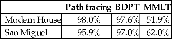
Figure 16.20 shows the contemporary house scene rendered with bidirectional path tracing and MMLT, using roughly equal computation time for each approach, and Figure 16.21 compares them with the San Miguel scene. For both, MMLT generates a better result, but the difference is particularly pronounced with the house scene, which is a particularly challenging scene for light transport algorithms in that there is essentially no direct illumination inside the house; all light-carrying paths must follow specular bounces through the glass windows. Table 16.1 helps illustrate these efficiency differences: for both of these scenes, both path tracing and BDPT have a lot of trouble finding paths that carry any radiance, while Metropolis is more effective at doing so thanks to path reuse.


Table 16.1
Percentage of Traced Paths That Carried Zero Radiance. With these two scenes, both path tracing and BDPT have trouble finding light-carrying paths: the vast majority of the generated paths don’t carry any radiance at all. Thanks to local exploration, Metropolis is better able to find additional light-carrying paths after one has been found. This is one of the reasons why it is more efficient than those approaches here.
| Path tracing | BDPT | MMLT | |
| Modern House | 98.0% | 97.6% | 51.9% |
| San Miguel | 95.9% | 97.0% | 62.0% |
16.4.3 Application to rendering
Metropolis sampling generates samples from the distribution of a given scalar function. To apply it to rendering, there are two issues that we must address: first, we need to estimate a separate integral for each pixel to turn the generated samples into an image, and, second, we need to handle the fact that L is a spectrally valued function but Metropolis needs a scalar function to compute the acceptance probability, Equation (13.7).
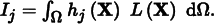
We can apply the ideas from Section 13.4.5 to use Metropolis samples to compute integrals. First, we define the image contribution function such that for an image with j pixels, each pixel Ij has a value that is the integral of the product of the pixel’s image reconstruction filter hj and the radiance L that contributes to the image:
The filter function hj only depends on the two components of X associated with the raster position. The value of hj for any particular pixel is usually 0 for the vast majority of samples X due to the filter’s finite extent.
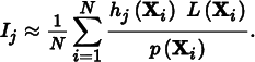
If N samples Xi are generated from some distribution, Xi ∼ p(X), then the standard Monte Carlo estimate of Ij is
Recall that Metropolis sampling requires a scalar function that defines the desired distribution of samples generated by the algorithm. Unfortunately, L is a spectrally valued function, and thus there is no unambiguous notion of what it means to generate samples proportional to L. To work around this issue, we will define a scalar contribution function I (X) that is used inside the Metropolis iteration. It is desirable that this function be large when L is large so that the distribution of samples has some relationship to the important regions of L. As such, using the luminance of the radiance value is a good choice for the scalar contribution function. In general, any function that is nonzero when L is nonzero will generate correct results, just possibly not as efficiently as a function that is more directly proportional to L.
Given a suitable scalar contribution function, I (X), Metropolis generates a sequence of samples Xi from I’s distribution, the normalized version of I :
and the pixel values can thus be computed as
The integral of I over the entire domain Ω can be computed using a traditional approach like bidirectional path tracing. If this value is denoted by b, with  , then each pixel’s value is given by

In other words, we can use Metropolis sampling to generate samples Xi from the distribution of the scalar contribution function I . For each sample, the pixels it contributes to (based on the extent of the pixel filter function h) have the value
added to them. Thus, brighter pixels have larger values than dimmer pixels due to more samples contributing to them (as long as the ratio Li (Xi)/I (Xi) is generally of the same magnitude).
16.4.4 Primary sample space sampler
The MLTIntegrator applies Metropolis sampling and MMLT to render images, using the bidirectional path tracer from Section 16.3. Its implementation is contained in the files integrators/mlt.h and integrators/mlt.cpp. Figure 16.22 shows the effectiveness of this integrator with a particularly tricky lighting situation. Before describing its implementation, we’ll first introduce the MLTSampler, which is responsible for managing primary sample space state vectors, mutations, and acceptance and rejection steps.

〈MLTSampler Declarations ≡
class MLTSampler : public Sampler {
public:
〈MLTSampler Public Methods 1030〉
protected:
〈MLTSampler Private Declarations 1030〉
〈MLTSampler Private Methods〉
〈MLTSampler Private Data 1030〉
};
The MLTIntegrator works best if the MLTSampler actually maintains three separate sample vectors—one for the camera subpath, one for the light subpath, and one for the connection step. We’ll say that these are three sample streams. The streamCount parameter to the constructor lets the caller request a particular number of such sample streams.
Later, during the initialization phase of MLTIntegrator, we will create many separate MLTSampler instances that are used to select a suitable set of starting states for the Metropolis sampler. Importantly, this process requires that each MLTSampler produces a distinct sequence of state vectors. The RNG pseudo-random number generator used by pbrt has a handy feature that makes this easy to accomplish: the RNG constructor accepts a sequence index, which selects between one of 263 unique pseudo-random sequences. We thus add an rngSequenceIndex parameter to the MLTSampler constructor that is used to supply a unique stream index to the internal RNG.
〈MLTSampler Public Methods〉 ≡ 1029
MLTSampler(int mutationsPerPixel, int rngSequenceIndex,
Float sigma, Float largeStepProbability, int streamCount)
: Sampler(mutationsPerPixel), rng(rngSequenceIndex), sigma(sigma),
argeStepProbability(largeStepProbability),
streamCount(streamCount) { }
The largeStepProbability parameter refers to the probability of taking a "large step” mutation, and sigma controls the size of "small step” mutations.
〈MLTSampler Private Data〉 ≡ 1029
RNG rng;
const Float sigma, largeStepProbability;
const int streamCount;
The MLTSampler::X member variable stores the current sample vector X. Because we generally don’t know ahead of time how many dimensions of X are actually needed during the sampler’s lifetime, we’ll start with an empty vector and expand it on demand as calls to MLTSampler::Get1D() and MLTSampler::Get2D() occur during rendering.
〈MLTSampler Private Data〉 + ≡ 1029
std::vector < PrimarySample > X;
The elements of this array have the type PrimarySample. The main task for PrimarySample is to record the current value of a single component of X on the interval [0, 1). In the following, we’ll add some additional functionality for representing proposed mutations and restoring the original sample value if a proposed mutation is rejected.
〈MLTSampler Private Declarations〉 ≡ 1029
struct PrimarySample {
Float value = 0;
〈PrimarySample Public Methods 1034〉
〈PrimarySample Public Data 1032〉
};
The Get1D() method returns the value of a single component of MLTSampler::X, whose position is given by GetNextIndex() —for now, we can think of this method as returning the value of a running counter that increases with every call. EnsureReady() expands MLTSampler::X as needed and ensures that its contents are in a consistent state. The details of these methods will be clearer after a few more preliminaries, so we won’t introduce their implementations just yet.
〈MLTSampler Method Definitions〉 ≡
Float MLTSampler::Get1D() {
int index = GetNextIndex();
EnsureReady(index);
return X[index].value;
}
The 2D analog simply performs two calls to Get1D().
〈MLTSampler Method Definitions〉 + ≡
Point2f MLTSampler::Get2D() {
return Point2f(Get1D(), Get1D());
}
Next, we will define several MLTIntegrator methods that are not part of the official Sampler interface. The first one, MLTSampler::StartIteration(), is called at the beginning of each Metropolis-Hastings iteration; it increases the currentIteration counter and determines which type of mutation (small or large) should be applied to the sample vector in the current iteration.
〈MLTSampler Method Definitions〉 + ≡
void MLTSampler::StartIteration() {
currentIteration++;
largeStep = rng.UniformFloat() < largeStepProbability;
}
currentIteration is a running counter, which keeps track of the current Metropolis-Hastings iteration index. Note that iterations with rejected proposals will be excluded from this count.
〈MLTSampler Private Data〉 + ≡ 1029
int64_t currentIteration = 0;
bool largeStep = true;
The MLTSampler::lastLargeStepIteration member variable records the index of the last iteration where a successful large step took place. Our implementation chooses the initial state X0 to be uniformly distributed on primary sample space [0, 1)∞; hence the first iteration’s state can be interpreted as the result of a large step in iteration 0.
〈MLTSampler Private Data〉 + ≡ 1029
int64_t lastLargeStepIteration = 0;
The MLTSampler::Accept() method is called whenever a proposal is accepted.
〈MLTSampler Method Definitions〉 + ≡
void MLTSampler::Accept() {
if (largeStep)
lastLargeStepIteration = currentIteration;
}
At this point, the main missing parts are MLTSampler::EnsureReady() and the logic that applies the actual mutations to MLTSampler::X. Before filling in those gaps, let us take a brief step back.
In theory, all entries in the X vector must be updated by small or large mutations in every iteration of the Metropolis sampler. However, doing so would sometimes be rather inefficient: consider the case where most iterations only query a small number of dimensions of X, hence MLTSampler::X has not grown to a large size yet. If a later iteration makes many calls to Get1D() or Get2D(), then the dynamic array MLTSampler::X must correspondingly expand, and these extra entries increase the cost of every subsequent Metropolis iteration (even if these components of X are never referenced again!).
Instead, it’s more efficient to update the PrimarySample entries on demand—that is, when they are referenced by an actual Get1D() or Get2D() call. Doing so avoids the aforementioned inefficiency, though after some period of inactivity, we must carefully replay all mutations that a given PrimarySample missed. To keep track of this information, an additional member variable recording the last iteration where a PrimarySample was modified is useful.
〈PrimarySample Public Data〉 ≡ 1030
int64_t lastModificationIteration = 0;
We now have enough background to proceed to the implementation of the MLTSampler::EnsureReady() method, which updates individual sample values when they are accessed.
〈MLTSampler Method Definitions〉 + ≡
void MLTSampler::EnsureReady(int index) {
〈Enlarge MLTSampler::X if necessary and get current X i 1032〉
〈ResetXi if a large step took place in the meantime 1032〉
〈Apply remaining sequence of mutations to sample 1033〉
}
First, any gaps are filled with zero-initialized PrimarySample s before a reference to the requested entry is obtained.
〈Enlarge MLTSampler::X if necessary and get current X i 〉 ≡ 1032
if (index > = X.size())
X.resize(index + 1);
PrimarySample &Xi = X[index];
When the last modification of Xi precedes the last large step, the current content of Xi.value is irrelevant, since it should have been overwritten with a new uniform sample in iteration lastLargeStepIteration. In this case, we simply replay this missed mutation and update the last modification iteration index accordingly.
〈ResetXi if a large step took place in the meantime〉 ≡ 1032
if (Xi.lastModificationIteration < lastLargeStepIteration) {
Xi.value = rng.UniformFloat();
Xi.lastModificationIteration = lastLargeStepIteration;
}
Next, a call to Backup() notifies the PrimarySample that a mutation is going to be proposed; doing so allows it to make a copy of Xi’s sample value in case the mutation is rejected. All remaining mutations between iterations lastLargeStepIteration and currentIteration are then applied. Two different cases can occur: when the current iteration is a large step, we simply initialize PrimarySample::value with a uniform sample. Otherwise, all iterations since the last large step are (by definition) small steps that we must replay.
〈Apply remaining sequence of mutations to sample〉 ≡ 1032
Xi.Backup();
if (largeStep) {
Xi.value = rng.UniformFloat();
} else {
int64_t nSmall = currentIteration - Xi.lastModificationIteration;
〈Apply nSmall small step mutations 1033〉
}
Xi.lastModificationIteration = currentIteration;
For small steps, we apply normally distributed perturbations to each component:
where σ is given by MLTIntegrator::sigma. The advantage of sampling with a normal distribution like this is that it naturally tries a variety of mutation sizes. It preferentially makes small mutations that remain close to the current state, which help locally explore the path space in small areas of high contribution where large mutations would tend to be rejected. On the other hand, because it also can make larger mutations, it also avoids spending too much time in a small part of the path space in cases where larger mutations have a good likelihood of acceptance.
Our implementation here merges the sequence of nSmall perturbations into a single update and clamps the result to the unit interval, wrapping around to the other end of the domain if necessary. Wrapping ensures that the transition probabilities for all pairs of sample values are symmetric.
〈Apply nSmall small step mutations〉 ≡ 1033
〈Sample the standard normal distribution N (0, 1) 1034〉
〈Compute the effective standard deviation and apply perturbation toXi 1034〉
Recall the rule that when two samples from normal distributions N(μ1, σ12) and N(μ2, σ22) are added, the sum is also normally distributed with parameters N(μ1 + μ2, σ12 + σ22). Thus, when n perturbations are to be applied to Xi, instead of performing n perturbations in sequence, it is equivalent and more efficient to directly sample

which we do by importance sampling a standard normal distribution and scaling the result by  . Applying the inversion method to the PDF

gives the following sampling method for a uniform sample ξ ∈ [0, 1):

where erf is the error function, erf  , and erf− 1 is its inverse. The ErfInv() function, not included here, approximates erf− 1 with a polynomial.
〈Sample the standard normal distribution N (0, 1)〉 ≡ 1033
Float normalSample = Sqrt2 * ErfInv(2 * rng.UniformFloat() - 1);
We scale the resulting sample by the effective variance from Equation (16.23) and use it to perturb the sample Xi before keeping only its fractional component, so that it remains in [0, 1).
〈Compute the effective standard deviation and apply perturbation toXi 〉 ≡ 1033
Float effSigma = sigma * std::sqrt((Float)nSmall);
Xi.value + = normalSample * effSigma;
Xi.value - = std::floor(Xi.value);
MLTSampler::Reject() must be called whenever a proposed mutation is rejected. It restores all PrimarySample s modified in the current iteration and reverts the iteration counter.
〈MLTSampler Method Definitions〉 + ≡
void MLTSampler::Reject() {
for (auto &Xi : X)
if (Xi.lastModificationIteration == currentIteration)
Xi.Restore();
--currentIteration;
}
The Backup() and Restore() methods make it possible to record the value of a Primary Sample before a mutation and to restore it if the mutation is rejected.
〈PrimarySample Public Methods〉 ≡ 1030
void Backup() {
valueBackup = value;
modifyBackup = lastModificationIteration;
}
void Restore() {
value = valueBackup;
lastModificationIteration = modifyBackup;
}
〈PrimarySample Public Data〉 + ≡ 1030
Float valueBackup = 0;
int64_t modifyBackup = 0;
Before wrapping up MLTSampler, we must address a detail that would otherwise cause issues when the sampler is used with BDPT. For each pixel sample, the BDPTIntegrator implementation calls GenerateCameraSubpath() and GenerateLightSubpath() in sequence to generate a pair of subpaths, each function requesting 1D and 2D samples from a supplied Sampler as needed.
In the context of MLT, the resulting sequence of sample requests creates a mapping between components of X and vertices on the camera or light subpath. With the process described above, the components X0, …, Xn determine the camera subpath (for some n ∈  ), and the remaining values Xn + 1, …, Xm determine the light subpath. If the camera subpath requires a different number of samples after a perturbation (e.g., because the random walk produced fewer vertices), then there is a shift in the assignment of primary sample space components to the light subpath. This leads to an unintended large-scale modification to the light path.
It is easy to avoid this problem with a more careful indexing scheme: the MLTSampler partitions X into multiple interleaved streams that cannot interfere with each other. The MLTSampler::StartStream() method indicates that subsequent samples should come from the stream with the given index. It also resets sampleIndex, the index of the current sample in the stream. (The number of such streams, MLTSampler::streamCount, is specified in the MLTSampler constructor.)
〈MLTSampler Method Definitions〉 + ≡
void MLTSampler::StartStream(int index) {
streamIndex = index;
sampleIndex = 0;
}
〈MLTSampler Private Data〉 + ≡ 1029
int streamIndex, sampleIndex;
After the stream is selected, the MLTSampler::GetNextIndex() method performs corresponding steps through the primary sample vector components. It interleaves the streams into the global sample vector—in other words, the first streamCount dimensions in X are respectively used for the first dimension of each of the streams, and so forth.
〈MLTSampler Public Methods〉 + ≡ 1029
int GetNextIndex() {
return streamIndex + streamCount * sampleIndex++;
}
16.4.5 MLT Integrator
Given all of this infrastructure—an explicit representation of an n-dimensional sample X, functions to apply mutations to it, and BDPT’s vertex abstraction layer for evaluating the radiance of a given sample value—we can move forward to the heart of the implementation of the MLTIntegrator.
〈MLT Declarations〉 ≡
class MLTIntegrator : public Integrator {
public:
〈MLTIntegrator Public Methods〉
private:
〈MLTIntegrator Private Data 1037〉
};
The MLTIntegrator constructor, not shown here, just initializes various member variables from parameters provided to it. These member variables will be introduced in the following as they are used.
We begin by defining the method MLTIntegrator::L(), which computes the radiance L(X) for a vector of sample values X provided by an MLTSampler. Its parameter depth specifies a specific path depth, and pRaster returns the raster position of the path, if the path successfully carries light from a light source to the film plane. The initial statement activates the first of three streams in the underlying MLTSampler.
〈MLT Method Definitions〉 ≡
Spectrum MLTIntegrator::L(const Scene &scene, MemoryArena &arena,
const std::unique_ptr < Distribution1D > &lightDistr,
MLTSampler &sampler, int depth, Point2f *pRaster) {
sampler.StartStream(cameraStreamIndex);
〈Determine the number of available strategies and pick a specific one 1036〉
〈Generate a camera subpath with exactly t vertices 1037〉
〈Generate a light subpath with exactly s vertices 1037〉
〈Execute connection strategy and return the radiance estimate 1037〉
}
The implementation uses three sample streams from the MLTSampler: the first two for the camera and light subpath and the third one for any Camera::Sample_Wi() or Light::Sample_Li() calls performed by connection strategies in ConnectBDPT() with s = 1 or t = 1 (refer to Section 16.3.3 for details).
〈MLTSampler Constants〉 ≡
static const int cameraStreamIndex = 0;
static const int lightStreamIndex = 1;
static const int connectionStreamIndex = 2;
static const int nSampleStreams = 3;
The body of MLTIntegrator::L() first selects an individual BDPT strategy for the provided depth value—this is the MMLT modification to PSSMLT—and invokes the bidirectional path-tracing machinery to compute a corresponding radiance estimate. For paths with zero scattering events (i.e., directly observed light sources), the only viable strategy provided by the underlying BDPT implementation entails intersecting them with a ray traced from the camera. For longer paths, there are depth + 2 possible strategies. The fragment below uniformly maps the first primary sample space dimension onto this set of strategies. The variables s and t denote the number of light and camera subpath sampling steps following the convention of the BDPTIntegrator.
〈Determine the number of available strategies and pick a specific one〉 ≡ 1036
int s, t, nStrategies;
if (depth == 0) {
nStrategies = 1;
s = 0;
t = 2;
} else {
nStrategies = depth + 2;
s = std::min((int)(sampler.Get1D() * nStrategies), nStrategies - 1);
t = nStrategies - s;
}
The next three fragments compute the radiance estimate. They strongly resemble BDPT with some MMLT-specific modifications: the first one samples a film position in [0, 1)2, maps it to raster coordinates, and tries to generate a corresponding camera subpath with exactly t vertices, failing with a 0-valued estimate for L when this was not possible.
〈Generate a camera subpath with exactly t vertices〉 ≡ 1036
Vertex *cameraVertices = arena.Alloc < Vertex > (t);
Bounds2f sampleBounds = (Bounds2f)camera- > film- > GetSampleBounds();
*pRaster = sampleBounds.Lerp(sampler.Get2D());
if (GenerateCameraSubpath(scene, sampler, arena, t, *camera,
*pRaster, cameraVertices) ! = t)
return Spectrum(0.f);
The camera member variable holds the Camera specified in the scene description file.
〈MLTIntegrator Private Data〉 ≡ 1035
std::shared_ptr < const Camera > camera;
The next fragment implements an analogous operation for the light subpath. Note the call to MLTSampler::StartStream(), which switches to the second stream of samples.
〈Generate a light subpath with exactly s vertices〉 ≡ 1036
sampler.StartStream(lightStreamIndex);
Vertex *lightVertices = arena.Alloc < Vertex > (s);
if (GenerateLightSubpath(scene, sampler, arena, s,
cameraVertices[0].time(),
*lightDistr, lightVertices) ! = s)
return Spectrum(0.f);
Finally, we switch to the last sample stream and invoke the (s, t) strategy via a call to ConnectBDPT(). The final radiance estimate is multiplied by the inverse probability of choosing the current strategy (s, t), which is equal to nStrategies.
〈Execute connection strategy and return the radiance estimate〉 ≡ 1036
sampler.StartStream(connectionStreamIndex);
return ConnectBDPT(scene, lightVertices, cameraVertices, s, t,
*lightDistr, *camera, sampler, pRaster) * nStrategies;
Main Rendering Loop
There are two phases to the rendering process implemented in MLTIntegrator::Render(). The first phase generates a set of bootstrap samples that are canidates for initial states of Markov chains and computes the normalization constant  , from Equation (16.22). The second phase runs a series of Markov chains, where each chain chooses one of the bootstrap samples for its initial sample vector and then applies Metropolis sampling.
〈MLT Method Definitions〉 + ≡
void MLTIntegrator::Render(const Scene &scene) {
std::unique_ptr < Distribution1D > lightDistr =
ComputeLightPowerDistribution(scene);
〈Generate bootstrap samples and compute normalization constant b 1038〉
〈Run nChains Markov chains in parallel 1039〉
〈Store final image computed with MLT 1042〉
}
Following the approach described in Section 13.4.3, we avoid issues with start-up bias by computing a set of bootstrap samples with a standard Monte Carlo estimator and using them to create a distribution that supplies the initial states of the Markov chains. This process builds on the sample generation and evaluation routines implemented previously.
Each bootstrap sample is technically a sequence of maxDepth + 1 samples with different path depths; the following fragment initializes the array bootstrapWeights with their corresponding luminance values. At the end, we create a Distribution1D instance to sample bootstrap paths proportional to their luminances and set the constant b to the sum of average luminances for each depth. Because we’ve kept the contributions of different path sample depths distinct, we can preferentially sample path lengths that make the largest contribution to the image. It is straightforward to compute the bootstrap samples in parallel, as all loop iterations are independent from one another.
〈Generate bootstrap samples and compute normalization constant b〉 ≡ 1038
int nBootstrapSamples = nBootstrap * (maxDepth + 1);
std::vector < Float > bootstrapWeights(nBootstrapSamples, 0);
std::vector < MemoryArena > bootstrapThreadArenas(MaxThreadIndex());
ParallelFor(
[&](int i) {
〈Generate ith bootstrap sample 1039〉
}, nBootstrap, 4096);
Distribution1D bootstrap(&bootstrapWeights[0], nBootstrapSamples);
Float b = bootstrap.funcInt * (maxDepth + 1);
As usual, maxDepth denotes the maximum number of interreflections that should be considered. nBootstrap sets the number of bootstrapping samples to use to seed the iterations and compute the integral of the scalar contribution function, Equation (16.22).
〈MLTIntegrator Private Data〉 + ≡ 1035
const int maxDepth;
const int nBootstrap;
In each iteration, we instantiate a dedicated MLTSampler with index rngIndex providing a unique sample vector that is uniformly distributed in the primary sample space. Next, we evaluate L to obtain a corresponding radiance estimate for the current path depth depth and write its luminance into bootstrapWeights. The raster-space position pRaster is not needed in the preprocessing phase, so it is ignored.
〈Generate ith bootstrap sample〉 ≡ 1038
MemoryArena &arena = bootstrapThreadArenas[ThreadIndex];
for (int depth = 0; depth < = maxDepth; ++depth) {
int rngIndex = i * (maxDepth + 1) + depth;
MLTSampler sampler(mutationsPerPixel, rngIndex, sigma,
largeStepProbability, nSampleStreams);
Point2f pRaster;
bootstrapWeights[rngIndex] =
L(scene, arena, lightDistr, sampler, depth, &pRaster).y();
arena.Reset();
}
The mutationsPerPixel parameter is analogous to Sampler::samplesPerPixel and denotes the number of iterations that MLT (on average!) spends in each pixel. Individual pixels will receive an actual number of samples related to their brightness, due to Metropolis’s property of taking more samples in regions where the function’s value is high. The total number of Metropolis samples taken is the product of the number of pixels and mutationsPerPixel.
The sigma and largeStepProbability member variables give the corresponding configuration parameters of the MLTSampler.
〈MLTIntegrator Private Data〉 + ≡ 1035
const int mutationsPerPixel;
const Float sigma, largeStepProbability;
We now move on to the main rendering task, which performs a total of nTotalMutations mutation steps spread out over nChains parallel Markov chains.
We must be careful that the actual number of mutation steps indeed comes out to be equal to nTotalMutations, particularly when nTotalMutations is not divisible by the number of parallel chains. The solution is simple: we potentially stop the last Markov chain a few iterations short; the corrected number of per-chain iterations is given by nChainMutations.
〈Run nChains Markov chains in parallel〉 ≡ 1038
Film &film = *camera- > film;
int64_t nTotalMutations = (int64_t)mutationsPerPixel *
(int64_t)film.GetSampleBounds().Area();
ParallelFor(
[&](int i) {
int64_t nChainMutations =
std::min((i + 1) * nTotalMutations / nChains,
nTotalMutations) - i * nTotalMutations / nChains;
〈Follow ith Markov chain for nChainMutations 1040〉
}, nChains);
nChains specifies the number of Markov chains that should be executed independently of each other. Its default value of 100 is a trade-off between providing sufficient parallelism and running each chain for a long amount of time.
〈MLTIntegrator Private Data〉 + ≡ 1035
const int nChains;
The MLT integrator only splats contributions to arbitrary pixels in the film; it doesn’t fill in well-defined tiles of the image plane. Therefore, a FilmTile isn’t necessary, and calls to Film::AddSplat() suffice to update the image.
〈Follow ith Markov chain for nChainMutations〉 ≡ 1039
MemoryArena arena;
〈Select initial state from the set of bootstrap samples 1040〉
〈Initialize local variables for selected state 1040〉
〈Run the Markov chain for nChainMutations steps 1041〉
Every Markov chain instantiates its own pseudo-random number generator following a unique stream. Note that this RNG instance is separate from the one in MLTSampler: it is used to pick the initial state and to accept or reject Metropolis proposals later on. Due to the ordering used earlier when initializing the entries of bootstrap array, we can immediately deduce the path depth of the sampled index bootstrapIndex. An important consequence of the method used to generate the bootstrap distribution is that the expected number of sampled initial states with a given depth value is proportional to their contribution to the image.
〈Select initial state from the set of bootstrap samples〉 ≡ 1040
RNG rng(i);
int bootstrapIndex = bootstrap.SampleDiscrete(rng.UniformFloat());
int depth = bootstrapIndex % (maxDepth + 1);
Having chosen the bootstrap sample, we must now obtain the corresponding primary sample space vector X. One way to accomplish this would have been to store all MLTSampler instances in the preprocessing phase. A more efficient approach builds on the property that the initialization in the MLTSampler constructor is completely deterministic and just depends on the rngSequenceIndex parameter. Thus, here we can create an MLTSampler with index bootstrapIndex, which recreates the exact same sampler that originally produced the sampled entry of the bootstrap distribution.
With the sampler in hand, we can compute the current value of L and its position on the film.
〈Initialize local variables for selected state〉 ≡ 1040
MLTSampler sampler(mutationsPerPixel, bootstrapIndex, sigma,
largeStepProbability, nSampleStreams);
Point2f pCurrent;
Spectrum LCurrent =
L(scene, arena, lightDistr, sampler, depth, &pCurrent);
The implementation of the Metropolis sampling routine in the following fragments follows the expected values technique from Section 13.4.1: a mutation is proposed, the value of the function for the mutated sample and the acceptance probability are computed, and the weighted contributions of both the new and old samples are recorded. The proposed mutation is then randomly accepted based on its acceptance probability.
One of the unique characteristics of MMLT (Section 16.4.2) compared to other Metropolis-type methods is that each Markov chain is restricted to paths of a fixed depth value. The first sample dimension selects among various different strategies, but only those producing equal path depths are considered, which improves performance of the method by making proposals more local. The contribution of all path depths is accounted for by starting many Markov chains with different initial states.
〈Run the Markov chain for nChainMutations steps〉 ≡ 1040
for (int64_t j = 0; j < nChainMutations; ++j)
{ sampler.StartIteration();
Point2f pProposed;
Spectrum LProposed =
L(scene, arena, lightDistr, sampler, depth, &pProposed);
〈Compute acceptance probability for proposed sample 1041〉
〈Splat both current and proposed samples to film 1041〉
〈Accept or reject the proposal 1042〉
}
Given the scalar contribution function’s value, the acceptance probability is then given by the simplified expression from Equation (13.8) thanks to the symmetry of our mutations on primary sample space.
As described at the start of the section, the spectral radiance value L(X) must be converted to a value given by the scalar contribution function so that the acceptance probability can be computed for the Metropolis sampling algorithm. Here, we compute the path’s luminance, which is a reasonable choice.
〈Compute acceptance probability for proposed sample〉 ≡ 1041
Float accept = std::min((Float)1, LProposed.y() / LCurrent.y());
Both samples can now be added to the image. Here, they are scaled with weights based on the expected values optimization introduced in Section 13.4.1.12
〈Splat both current and proposed samples to film〉 ≡ 1041
if (accept > 0)
film.AddSplat(pProposed, LProposed * accept / LProposed.y());
film.AddSplat(pCurrent, LCurrent * (1 - accept) / LCurrent.y());
Finally, the proposed mutation is either accepted or rejected, based on the computed acceptance probability accept. If the mutation is accepted, then the values pProposed and LProposed become properties of the current state. In either case, the MLTSampler must be informed of the outcome so that it can update the PrimarySample accordingly.
〈Accept or reject the proposal〉 ≡ 1041
if (rng.UniformFloat() < accept) {
pCurrent = pProposed;
LCurrent = LProposed;
sampler.Accept();
} else
sampler.Reject();
Metropolis sampling only considers the relative frequency of samples and cannot create an image that is correctly scaled in absolute terms; hence the value b is crucial: it contains an estimate of the average luminance of the Film that we use to remove this ambiguity. Each Metropolis iteration within 〈Run nChains Markov chains in parallel〉 has splatted contributions with weighted unit luminance to the Film so that the final average film luminance before Film::WriteImage() is exactly equal to mutationsPerPixel. We thus must cancel this factor out and multiply by b when writing the image to convert to actual incident radiance on the film.
〈Store final image computed with MLT〉 ≡ 1038
camera- > film- > WriteImage(b / mutationsPerPixel);
Further reading
The general idea of tracing light-carrying paths from light sources was first investigated by Arvo (1986), who stored light in texture maps on surfaces and rendered caustics. Heckbert (1990b) built on this approach to develop a general ray-tracing-based global illumination algorithm, and Pattanaik and Mudur (1995) developed an early particletracing technique. Christensen (2003) surveyed applications of adjoint functions and importance to solving the LTE and related problems.
Sources of non-symmetric scattering and their impact on bidirectional light transport algorithms were first identified by Veach (1996).
Pharr and Humphreys (2004) proposed the method to sample emitted rays from environment map light sources that is used in this chapter. Dammertz and Hanika (2009) described a variation on this approach that sampled points on the visible faces of the scene bounding box rather than an oriented disk; this can lead to fewer wasted samples.
Photon Mapping
Approaches like Arvo’s caustic rendering algorithm (Arvo 1986) formed the basis for an improved technique that stored illumination in texture maps on surfaces developed by Collins (1994). Density estimation techniques for global illumination were first introduced by Shirley, Walter, and collaborators (Shirley et al. 1995; Walter et al. 1997).
Jensen (1995, 1996) developed the photon mapping algorithm, which introduced the key innovation of storing the light contributions in a general 3D data structure rather than in texture maps. Important improvements to the photon mapping method are described in follow-up papers and a book by Jensen (1996, 1997, 2001).
Final gathering for finite-element radiosity algorithms was first described in Reichert’s thesis (Reichert 1992). If the full photon map is stored in memory, the directional distribution of photons can be used to construct optimized final gathering techniques that importance sample directions that are likely to have large contributions (Jensen 1995). More recently, Spencer and Jones (2009a) described how to build a hierarchical kd-tree of photons such that traversal could be stopped at higher levels of the tree and showed that using the footprints of final gather rays computed using ray differentials can lead to better results than the usual approach. In another paper, Spencer and Jones (2009b) showed that a simple iterative relaxation scheme to reduce clumping in photon maps can lead to dramatic improvements in the quality of density estimates.
Havran et al. (2005) developed a final gathering photon mapping algorithm based on storing final gather intersection points in a kd-tree in the scene and then shooting photons from the lights; when a photon intersects a surface, the nearby final gather intersection records are found and the photon’s energy can be distributed to the origins of the corresponding final gather rays. Herzog et al. (2007) described an approach based on storing all of the visible points as seen from the camera and splatting photon contributions to them. Hachisuka et al. (2008b) developed the progressive photon mapping algorithm; stochastic progressive photon mapping was developed by Hachisuka and Jensen (2009).
The advantages of SPPM over traditional photon mapping are significant, and the approach was quickly adopted after its introduction. Hachisuka et al. (2010) showed how to use arbitrary density estimation kernels and how to compute error estimates during rendering to automatically determine when to stop further iterations. Knaus and Zwicker (2011) re-derived SPPM following a different approach and showed that it was possible to only maintain global statistics for values like the current search radius rather than having a separate value for each pixel. See Kaplanyan and Dachsbacher (2013a) for an extensive study of SPPM’s convergence rates and an improved (but more complex) method for updating SPPM estimates after each iteration.
The question of how to find the most effective set of photons for photon mapping is an important one: light-driven particle-tracing algorithms don’t work well for all scenes (consider, for example, a complex building model with lights in every room but where the camera sees only a single room). The earliest applications of Metropolis sampling to photon mapping was proposed in Wald’s Diploma thesis (1999). Fan et al. (2005) showed that the application of Veach’s particle-tracing theory to photon mapping provides a mechanism for generating photon paths starting from the camera. They were able to use this approach in conjunction with a Metropolis sampling algorithm to generate photon distributions. Hachisuka and Jensen (2011) used Metropolis sampling to find photon paths that were visible to the camera; their algorithm is notable for both its effectiveness and its ease of implementation. Chen et al. (2011) use a similar approach but sample additional terms of the path contribution function and distribute additional photons to parts of the image with higher error.
Jensen and Christensen (1998) were the first to generalize the photon mapping algorithm to participating media. Knaus and Zwicker (2011) showed how to render participating media using SPPM. Jarosz et al. (2008) had the important insight that expressing the scattering integral over a beam through the medium as the measurement to be evaluated could make photon mapping’s rate of convergence much higher than if a series of point photon estimates was instead taken along each ray. Section 5.6 of Hachisuka’s thesis Knaus and Zwicker (2011) and Jarosz et al. (2011a, 2011b) showed how to apply this approach progressively. For another representation, see Jakob et al. (2011), who fit a sum of anisotropic Gaussians to the equilibrium radiance distribution in participating media.
Bidirectional Path Tracing
Bidirectional path tracing was independently developed by Lafortune and Willems (1994) and Veach and Guibas (1994). The development of multiple importance sampling was integral to the effectiveness of bidirectional path tracing (Veach and Guibas 1995). Lafortune and Willems (1996) showed how to apply bidirectional path tracing to rendering participating media, and Kollig and Keller (2000) showed how bidirectional path tracing can be modified to work with quasi-random sample patterns.
An exciting recent development has been simultaneous work by Hachisuka et al. (2012) and Georgiev et al. (2012), who developed a unified framework for both photon mapping and bidirectional path tracing. Their approaches allowed photon mapping to be included in the path space formulation of the light transport equation, which in turn made it possible to derive light transport algorithms that use both approaches to generate paths and combine them using multiple importance sampling.
Kaplanyan and Dachsbacher (2013b) noted that photon mapping algorithms use illumination from nearby points even in cases where unbiased approaches are effective. They developed a technique for regularization of light-carrying paths, where an unbiased path tracer or bidirectional path tracer is modified to treat delta distributions that cause impossible-to-sample configurations instead as having non-zero value over a small cone of directions. Thus, bias is introduced only in the challenging settings.
Vorba et al. (2014) developed an approach to compute effective sampling distributions for difficult lighting configurations over the course of rendering rather than in a preprocess and showed its applicability to bidirectional path tracing.
Metropolis Light Transport
Veach and Guibas (1997) first applied the Metropolis sampling algorithm to solving the light transport equation. They demonstrated how this method could be applied to image synthesis and showed that the result was a light transport algorithm that was robust to traditionally difficult lighting configurations (e.g., light shining through a slightly ajar door). Pauly, Kollig, and Keller (2000) generalized the MLT algorithm to include volume scattering. Pauly’s thesis (Pauly 1999) described the theory and implementation of bidirectional and Metropolis-based algorithms for volume light transport.
Fan et al. (2005) developed a method that let the user explicitly specify a number of important paths (e.g., through a tricky geometric configuration) that could then be used as a target state in Metropolis mutations. The energy redistribution path tracing algorithm by Cline et al. (2005) starts one or more Markov chains at every pixel of the image and runs them for a small number of iterations; the method is notable for being unbiased despite its use of non-ergodic Markov chains that can only explore a subset of path space.
Hoberock’s Ph.D. dissertation discusses a number of alternatives for the scalar contribution function, including those that adapt the sampling density to pay more attention to particular modes of light transport and those that focus on reducing noise in the final image (Hoberock 2008).
Kelemen et al. (2002) developed the "primary sample space MLT” formulation of Metropolis light transport. They also suggested the approach implemented in the MLTSampler for lazily updating sample vector components when performing mutations. Hachisuka et al. (2014) developed the MMLT approach that is implemented in the MLTIntegrator in this chapter.
The optimal choice of the large step probability is scene dependent: for scenes with difficult-to-sample transport paths, it’s better for it to be lower, so that more successful mutations are performed with small steps once a good path is found. For scenes with simpler light transport, it’s better for the probability to be higher, so that the overall path space is explored more thoroughly. Zsolnai and Szirmay-Kalos (2013) developed a technique that gathered statistics about paths during the bootstrap phase that made it possible to automatically set this parameter to a near-optimal value.
Other Rendering Approaches
A number of algorithms have been developed based on a first phase of computation that traces paths from the light sources to create "virtual lights,” where these lights are then used to approximate indirect illumination during a second phase. The principles behind this approach were first introduced by Keller’s work on instant radiosity (1997). The more general instant global illumination algorithm was developed by Wald, Benthin, and collaborators (Wald et al. 2002, 2003; Benthin et al. 2003). See Dachsbacher et al.’s recent survey article (2014) for a summary of recent work in this area.
Building on the virtual point lights concept, Walter and collaborators (2005, 2006) developed lightcuts, which are based on creating thousands of virtual point lights and then building a hierarchy by progressively clustering nearby ones together. When a point is being shaded, traversal of the light hierarchy is performed by computing bounds on the error that would result from using clustered values to illuminate the point versus continuing down the hierarchy, leading to an approach with both guaranteed error bounds and good efficiency.
Bidirectional lightcuts (Walter et al. 2012) trace longer subpaths from the camera to obtain a family of light connection strategies; combining the strategies using multiple importance sampling eliminates bias artifacts that are commonly produced by virtual point light methods.
Jakob and Marschner (2012) expressed light transport involving specular materials as an integral over a high-dimensional manifold embedded in path space. A single light path corresponds to a point on the manifold, and nearby paths are found using a local parameterization that resembles Newton’s method; they applied a Metropolis-type method through this parameterization to explore the neighborhood of challenging specular and near-specular configurations.
Hanika et al. (2015a) apply an improved version of the local path parameterization in a pure Monte Carlo context to estimate the direct illumination through one or more dielectric boundaries; this leads to significantly better convergence when rendering glass-enclosed objects or contaminated surfaces with water droplets.
Kaplanyan et al. (2014) observed that the path contribution function is close to being separable when paths are parameterized using the endpoints and the half-direction vectors at intermediate vertices, which are equal to the microfacet normals in the context of microfacet reflectance models. Performing Metropolis sampling in this half-vector domain leads to a method that is particularly good at rendering glossy interreflection. An extension by Hanika et al. (2015b) improves the robustness of this approach and proposes an optimized scheme to select mutation sizes to reduce sample clumping in image space.
Another interesting approach was developed by Lehtinen and collaborators (Lehtinen et al. 2013, Manzi et al. 2014). Building on the observation that ideally, most samples from the path space should be taken around discontinuities (and not in smooth regions of the image), they developed a measurement contribution function for Metropolis sampling that focused samples on gradients in the image. They then reconstructed high-quality final images from horizontal and vertical gradient images and a coarse, noisy image. More recently, Kettunen et al. (2015) showed how this approach could be applied to regular path tracing, without Metropolis sampling. Manzi et al. (2015) showed its application to bidirectional path tracing.
Hair is particularly challenging to render; not only is it extremely geometrically complex but multiple scattering among hair also makes a significant contribution to its final appearance. Traditional light transport algorithms often have difficulty handling this case well. See the papers by Moon and Marschner (2006), Moon et al. (2008), and Zinke et al. (2008) for recent work in specialized rendering algorithms for hair.
While the rendering problem as discussed so far has been challenging enough, Jarabo et al. (2014a) showed the extension of the path integral to not include the steady-state assumption—i.e., accounting for the non-infinite speed of light. Time ends up being extremely high frequency, which makes rendering challenging; they showed successful application of density estimation to this problem.
Exercises
 16.1 Derive importance functions and implement the Camera We(), Pdf_We(), Sample_Wi(), and Pdf_Wi() methods for one or more of EnvironmentCamera, OrthographicCamera, or RealisticCamera. Render images using bidirectional path tracing or MMLT and show that given sufficient samples, they converge to the same images as when the scene is rendered with standard path tracing.
16.2 Discuss situations where the current methods for sampling outgoing rays from ProjectionLight s and GonioPhotometricLight s may be extremely inefficient, choosing many rays in directions where the light source casts no illumination. Use the Distribution2D structure to implement improved sampling techniques for each of them based on sampling from a distribution based on the luminance in their 2D image maps, properly accounting for the transformation from the 2D image map sampling distribution to the distribution of directions on the sphere. Verify that the system still computes the same images (modulo variance) with your new sampling techniques when using an Integrator that calls these methods. Determine how much efficiency is improved by using these sampling methods instead of the default ones.
 16.3 Implement Walter et al.’s lightcuts algorithm in pbrt (Walter et al. 2005, 2006). How do the BSDF interfaces in pbrt need to be generalized to compute the error terms for lightcuts? Do other core system interfaces need to be changed? Compare the efficiency of rendering images with global illumination using your implementation to some of the other bidirectional integrators.
 16.4 Experiment with the parameters to the SPPMIntegrator until you get a good feel for how they affect rendering time and the appearance of the final image. At a minimum, experiment with varying the search radius, the number of photons traced, and the number of iterations.
16.5 Another approach to improving the efficiency of photon shooting is to start out by shooting photons from lights in all directions with equal probability but then to dynamically update the probability of sampling directions based on which directions lead to light paths that have high throughput weight and end up being used by visible points. Photons then must be reweighted based on the probability for shooting a photon in a particular direction. (As long as there is always nonzero possibility of sending a photon in any direction, this approach doesn’t introduce additional bias into the shooting algorithm.) Derive and implement such an approach. Show that in the limit, your modified SPPMIntegrator computes the same results as the original. How much do these changes improve the rate of convergence?
16.6 The SPPMIntegrator ends up storing all of the BSDFs along camera paths to the first visible point, even though only the last BSDF is needed. First, measure how much memory is used to store unnecessary BSDFs in the current implementation for a variety of scenes. Next, modify the VisiblePoint representation to store the reflectance, BSDF::rho(), at visible points and then compute reflection assuming a Lambertian BSDF. Does this approximation introduce visible error in test scenes? How much memory is saved?
16.7 To find the VisiblePoint s around a photon-surface intersection, the SPPM Integrator uses a uniform grid to store the bounding boxes of visible points expanded by their radii. Investigate other spatial data structures for storing visible points that support efficient photon/nearby visible point queries, and implement an alternate approach. (You may want to specifically consider octrees and kd-trees.) How do performance and memory use compare to the current implementation?
16.8 Implement "final gathering” in the SPPMIntegrator, where camera rays are followed for one more bounce after hitting a diffuse surface. Investigate how many iterations and how many photons per iteration are needed to get good results with this approach for a variety of scenes compared to the current implementation.
16.9 There is actually one case where collisions from the hash() function used by the SPPMIntegrator can cause a problem: if, for example, nearby voxels have a collision, then a VisiblePoint that overlaps both of them will be placed in a linked list twice, and then a photon that is close to them will incorrectly contribute to the pixel’s value twice. Can you prove that this will never happen for the current hash function? If it does happen, can you construct a scene where the error makes a meaningful difference in the final image? How might this problem be addressed?
16.10 Extend the SPPM integrator to support volumetric scattering. First, read the papers by Knaus and Zwicker (2011) and Jarosz et al. (2011b) and choose one of these approaches. Compare the efficiency and accuracy of images rendered with your implementation to rendering using the bidirectional path tracer or the MMLT integrator.
16.11 One shortcoming of the current SPPMIntegrator implementation is that it’s inefficient for scenes where the camera is only viewing a small part of the over- all scene: many photons may need to be traced to find ones that are visible to the camera. Read the paper by Hachisuka and Jensen (2011) on using adaptive Markov chain sampling to generate photon paths and implement their approach. Construct a scene where the current implementation is inefficient and your new one does much better, and render comparison images using equal amounts of computation for each. Are there any scenes where your implementation computes worse results?
16.12 Extend the BDPT integrator to support subsurface scattering with BSSRDFs. In addition to connecting pairs of vertices by evaluating the geometric term and BSDFs, your modified integrator should also evaluate the BSSRDF S(po, ωo, pi, ωi) when two points are located on an object with the same Material with a non- nullptr -valued BSSRDF. Since two connection techniques lead to paths with a fundamentally different configuration—straight-line transport versus an additional subsurface scattering interaction on the way from pi on po—their area product density should never be compared to each other when computing multiple importance sampling weights.
16.13 Implement Russian roulette to randomly skip tracing visibility rays for low-contribution connections between subpaths in the ConnectBDPT() function. Measure the change in Monte Carlo efficiency compared to the current BDPTIntegrator implementation.
16.14 Modify the BDPT integrator to use the path space regularization technique described by Kaplanyan and Dachsbacher (2013b). (Their method makes it possible for light transport algorithms based on incremental path construction to still handle difficult sampling cases based on chains of specular interactions.) Construct a scene where this approach is useful, and render images to compare results between this approach, SPPM, and an unmodified bidirectional path tracer.
16.15 By adding mutation strategies that don’t necessarily modify all of the sample values Xi, it can be possible to reuse some or all of the paths generated by the previous samples in the MLTIntegrator. For example, if only the PrimarySample values for the light subpath are mutated, then the camera subpath can be reused. (An analogous case holds for the light subpath.) Even if a mutation is proposed for a subpath, if the samples for its first few vertices are left unchanged, then that portion of the path doesn’t need to be retraced.
Modify the MLTIntegrator to add one or more of the above sampling strategies, and update the implementation so that it reuses any partial results from the previous sample that remain valid when your new mutation is used. You may want to add both "small step” and "large step” variants of your new mutation. Compare the mean squared error of images rendered by your modified implementation to the MSE of images rendered by the original implementation, comparing to a reference image rendered with a large number of samples. For the same number of samples, your implementation should be faster but will likely have slightly higher error due to additional correlation among samples. Is the Monte Carlo efficiency of your modified version better than the original implementation?
16.16 In his Ph.D. dissertation, Hoberock proposes a number of alternative scalar contribution functions for Metropolis light transport, including ones that focus on particular types of light transport and ones that adapt the sample density during rendering in order to reduce perceptual error (Hoberock 2008). Read Chapter 6 of his thesis, and implement either the multistage MLT or the noise-aware MLT algorithm that he describes.