Supervised regression/classification methods learn a model of relation between the target vectors  and the corresponding input vectors
  consisting of N training samples and utilize this model to predict/classify target values for the previously unseen inputs.
In real-world data, the presence of noise (in regression) and class overlap (in classification) implies that the principal modeling challenge is to avoid “overfitting” of the training set, which is an important concern with this modeling.
Unlike traditional neural network approaches which suffer difficulties with generalization, producing models that may overfit the data, SVMs [43] are a popular machine learning approach for classification, regression, and other learning tasks, based on statistical learning theory (Vapnik–Chervonenkis or VC-theory).
At a sufficiently high dimension, patterns are orthogonal to each other, and thus it is easier to find a separating hyperplane for data in a high dimension space.
Not all patterns are necessary for finding a separating hyperplane. In fact, it is sufficient to use only those points that are near the boundary between groups to construct the boundary.
As a kind of generalization intelligence, this chapter presents SVMs together with applications in target regression and classification.
8.1 Support Vector Machines: Basic Theory
Support vector machines comprise a new class of learning algorithms, originally developed for pattern recognition [3, 46], and motivated by results of statistical learning theory [43].
The problem of empirical data modeling is germane to many engineering applications. In empirical data modeling a process of induction is used to build up a model of the system under study, and it is hoped to deduce responses of the system that have yet to be observed.
The SVMs aim at minimizing an upper bound of the generalization error by maximizing the margin between the separating hyperplane1 and the data. What makes SVMs attractive is the property of condensing information in the training data and providing a sparse representation by using a very small number of data points (support vectors, SVs) [17].
8.1.1 Statistical Learning Theory
This subsection is a very brief introduction to statistical learning theory [42, 44].
Statistical learning theory based modeling aims at choosing a model from the hypothesis space, which is closest (with respect to some error measure) to the underlying function in the target space.
Approximation Error is a consequence of a poor choice of the hypothesis space smaller than the target space, which will result in a large approximation error, and is referred to as model mismatch.
Estimation Error is the error due to the learning procedure which results in a technique selecting the non-optimal model from the hypothesis space.
In order to choose the best available approximation to the supervisor’s response, it is important to measure the loss or discrepancy L(y, f(w, x)) between the response y of the supervisor to a given input x and the response f(w, x) provided by the learning machine.
 . We would like to find the function f such that the expected value of the loss, called the risk function, is minimized:

The problem is: the joint probability distribution P(x, y) = P(y|x)P(x) is unknown, and the only available information is contained in the training set 
 .
.

 . In the above equation, the Boolean function f(w, x
i) on the input feature x
i and a set of Boolean functions on the input features {f(w, x
i), w ∈ W, x
i ∈ X} are known as hypothesis and hypothesis space, respectively.
. In the above equation, the Boolean function f(w, x
i) on the input feature x
i and a set of Boolean functions on the input features {f(w, x
i), w ∈ W, x
i ∈ X} are known as hypothesis and hypothesis space, respectively.
Empirical risk minimization (ERM) principle is to minimize R
emp(w) over the set w ∈ W, results in a risk  which is close to its minimum.
- 1.Does the empirical risk R emp(w) converge uniformly to the actual risk R(w) over the full set f(w, x), w ∈ W, namely
 (8.1.3)
 - 2.
What is the rate of convergence?
The theory of uniform convergence of empirical risk to actual risk includes necessary and sufficient conditions as well as bounds for the rate of convergence. These bounds independent of the distribution function P(x, y) are based on the Vapnik–Chervonekis (VC) dimension of the set of functions f(w, x) implemented by the learning machine.
For a set of functions {f(w)}, w is a generic set of parameters: a choice of w specifies a particular function and can be defined for various classes of function f.
Let us consider only the functions corresponding to the two-class pattern recognition case, so that f(w, x) ∈{−1, 1}, ∀w, x.
If a given set of N data points can be labeled in all possible 2N ways, and for each labeling, a member of the set {f(w)} with correctly assigned labels can be found, then the set of points is said to be shattered by the set of functions.
 , and the set {f(w)} consists of oriented straight lines, so that for a given line, all points on one side are assigned to the class 1, and all points on the other side, the class − 1, as shown in Fig. 8.1.
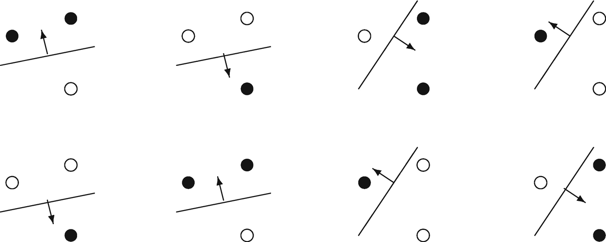
Three points in  , shattered by oriented lines. The arrow points to the side with the points labeled black
One can find at least one set of 3 points in 2D all of whose 23 = 8 possible labeling can be separated by some hyperplane. The orientation is shown by an arrow, specifying on which side of the line points is to be assigned the label 1. Any set of 4 points, all of whose 24 = 16 possible labeling, are not separable by hyperplanes.
Suppose we have a data set containing N points. These N points can be labeled in 2N ways as positive “+” and negative “−.” Therefore, 2N different learning problems can be defined by N data points. If for any of these problems, we can find a hypothesis  that separates the positive examples from the negative, then we say
  shatters N points. That is, any learning problem definable by N examples can be learned without error by a hypothesis drawn from
  .
.
 be a 2n full factorial design with levels − 1 and + 1, and a fractional factorial design
  be a subset of
  . The indicator function F of its fraction
  is a function defined on
  as follows:
The VC-dimension of a set of indicator functions f(w, x), w ∈ W is the maximal number h of vectors which can be shattered in all possible 2h ways by f(w, x), w ∈ W.
For example, h = n + 1 for linear decision rules in n-dimensional space, since they can shatter at most n + 1 points.
It is well-known [45] that the finiteness of the VC-dimension of the set of indicator functions implemented by the learning machine forms the necessary and sufficient condition for consistency of the ERM method independent of probability measure. Finiteness of VC-dimension also implies fast convergence.
Consider some set of m points in
 . Choose any one of the points as origin. Then the m points can be shattered by oriented hyperplanes if and only if the position vectors of the remaining points are linearly independent.
The VC-dimension of the set of oriented hyperplanes in  is n + 1, since we can always choose n + 1 points, and then choose one of the points as origin, such that the position vectors of the remaining n points are linearly independent, but can never choose n + 2 such points (since no n + 1 vectors in
  can be linearly independent).
8.1.2 Linear Support Vector Machines
We discuss linear SVMs in two cases: the separable case and the nonseparable case.
Consider first the simplest case: linear machines trained on separable data. We are given the labeled training data  with
with  . Suppose we have a “separating hyperplane” which separates the positive from the negative data samples. The points x on the hyperplane satisfy w
Tx + b = 0, where w is normal to the hyperplane,
. Suppose we have a “separating hyperplane” which separates the positive from the negative data samples. The points x on the hyperplane satisfy w
Tx + b = 0, where w is normal to the hyperplane,  is the perpendicular distance from the hyperplane to the origin, and
  is the Euclidean norm of w.
Two sets of points in
 may be separated by a hyperplane if and only if the intersection of their convex hulls is empty.
Let  and
and  be the shortest distances from the separating hyperplane to the closest positive and negative data samples, respectively. Then, the “margin” of a separating hyperplane can be defined to be
  .
.
 . For this end, all the training data need to satisfy the following constrains:


Clearly, the points satisfying the equality in (8.1.5) lie on the hyperplane  with normal w and perpendicular distance from the origin
  . Similarly, the points satisfying the equality in Eq. (8.1.6) lie on the hyperplane
  with normal again w and perpendicular distance from the origin
  . Then
  and hence the margin is simply 2∕∥w∥2.
 and
and  are parallel, and no training points fall between them. Thus the pair of hyperplanes (H
1, H
2) which gives the maximum margin can be found by minimizing
are parallel, and no training points fall between them. Thus the pair of hyperplanes (H
1, H
2) which gives the maximum margin can be found by minimizing  subject to constraints (8.1.7), namely we have the constrained optimization problem:


 .
.


For an error to occur, the corresponding  must exceed unity, so
  is an upper bound on the number of training errors. Hence, a natural way to assign an extra cost for errors is to change the objective function to be minimized from
  to
to  , where C is a parameter to be chosen by the user, a larger C corresponding to assigning a higher penalty to errors.


8.2 Kernel Regression Methods
Following the development of support vector machines, positive definite kernels have recently attracted considerable attention in the machine learning community.
8.2.1 Reproducing Kernel and Mercer Kernel
Consider how a linear SVM is generalized to the case where the decision function f(x), whose sign represents the class assigned to data point x, is not a linear function of the data x?
 of real-valued function on a compact domain X with the reproducing property that for
  , and each x ∈ X, there exists M
x, not depending on f such that
, and each x ∈ X, there exists M
x, not depending on f such that
![$$\displaystyle \begin{aligned} \mathbb{F}_x[f]=|f(\mathbf{x})|=\langle f(\cdot ),K_x (\cdot )\rangle\leq M_x\|f\|,\quad \forall~ f\in \mathbb{H}, \end{aligned} $$](../images/492994_1_En_8_Chapter/492994_1_En_8_Chapter_TeX_Equ27.png)
![$$\mathbb {F}_x[f]$$](../images/492994_1_En_8_Chapter/492994_1_En_8_Chapter_TeX_IEq49.png) is called the evaluation functional of f. That is to say,
is called the evaluation functional of f. That is to say, ![$$\mathbb {F}_x[f]$$](../images/492994_1_En_8_Chapter/492994_1_En_8_Chapter_TeX_IEq50.png) is a bounded linear functional.
is a bounded linear functional.
The reproducing property above states that the inner product of a function f and a kernel function K x, 〈f(⋅), K x(⋅)〉, is f(x) in the RKHS. Because K x must ensure reproducing the function f, the function K x(⋅) is called the reproducing kernel of f for the RKHS H.

 ∈ X, where X is a closed subset of
  . The N × N matrix K with entries
 .
.
 , and
, and  a symmetric function satisfying: for any finite set of points
  in X and real numbers
  ,
, 
 , then positive definition (pd) kernels have the following general properties:
 - 1.
If K 1, …, K n are p.d. kernels and λ 1, …, λ n ≥ 0, then the sum
 is p.d.
 - 2.
If K 1, …, K n are p.d. kernels and α 1, …, α n ∈{1, …, N}, then their product
 is p.d.
 - 3.
For a sequence of p.d. kernels, the limit K =limn→∞K n is p.d., if the limit exists.
- 4.
If X 0 ⊆ X, then
 is also a p.d. kernel.
 - 5.If
 is a sequence of p.d. kernels, then
  is p.d. kernel on X
1 ×⋯ × X
n.
is p.d. kernel on X
1 ×⋯ × X
n. is p.d. kernel on X
1 ×⋯ × X
n.
is p.d. kernel on X
1 ×⋯ × X
n.
- 1.
For every y, K(x, y) as function of x belongs to F.
- 2.The reproducing property: for every y ∈ E and every f ∈ F,
 (8.2.5)
Here the subscript x ∗ by the scalar product indicates that the scalar product applies to functions of x.
 be positive defined. Then, there must be a unique RKHS
  whose reproducing kernel is K(x, y). Moreover, if the space
  has the inner product

where
 and
and
 , then
 is an effective RKHS.
Moore–Aronszajn theorem states that there is one-to-one correspondence between positive definite kernel function K(x, y) and RKHS  . This is why the kernel function is limited to the reproducing kernel Hilbert space
  .
.
Uniqueness. If a reproducing kernel K(x, y) exists, then it is unique.
Existence. For the existence of a reproducing kernel K(x, y) it is necessary and sufficient that for every y of the set E, f(y) be a continuous functional of f running through the Hilbert space F.
Positiveness.
![$$\mathbf {K}=[K({\mathbf {x}}_i,{\mathbf {y}}_j)]_{i,j=1}^{n,n}$$](../images/492994_1_En_8_Chapter/492994_1_En_8_Chapter_TeX_IEq73.png) is a positive matrix in the sense of E.
is a positive matrix in the sense of E.One-to-one correspondence. To every positive matrix
![$$\mathbf {K}=[K({\mathbf {x}}_i,{\mathbf {y}}_j)]_{{i,j}=1}^{n,n}$$](../images/492994_1_En_8_Chapter/492994_1_En_8_Chapter_TeX_IEq74.png) , there corresponds one and only one class of functions with a uniquely determined quadratic form in it, forming a Hilbert space and admitting K(x, y) as a reproducing kernel.
, there corresponds one and only one class of functions with a uniquely determined quadratic form in it, forming a Hilbert space and admitting K(x, y) as a reproducing kernel.Convergence. If the class F possesses a reproducing kernel K(x, y), every sequence of functions {f n} which converges strongly to a function f in the Hilbert space F, converges also at every point in the ordinary sense,
 .
.
The following Mercer’s theorem provides a construction method of the nonlinear reproducing kernel function.


![$${\boldsymbol \phi }(\mathbf {x})=[\phi _1^{\,} (\mathbf {x}),\ldots ,\phi _M^{\,} (\mathbf {x})]^T$$](../images/492994_1_En_8_Chapter/492994_1_En_8_Chapter_TeX_IEq76.png) is a nonlinear function.
is a nonlinear function.


 is an N × 1 summation vector with all entries equal to 1.
- 1.
Kernel PCA: For given data vectors
 and an RBF kernel, K dominant eigenvalues and their corresponding eigenvectors of the kernel matrix K give the kernel PCA after the principal components in standard PCA are replaced by the principal components of the kernel matrix K. The kernel PCA was originally proposed by Schölkopf et al. [33].
- 2.
Kernel K-means clustering: If there are K distinct clustered regions within the N data samples, then there will be K dominant terms
 that provide a means of estimating the possible number of clusters within the data sample in kernel based K-means clustering [16].
Kernel PCA is a nonlinear generalization of PCA in the sense that it is performing PCA in feature spaces of arbitrarily large (possibly infinite) dimensionality. If the kernels  are used, then the kernel PCA reduces to standard PCA. Compared to the standard PCA, kernel PCA has the main advantage that no nonlinear optimization is involved; it is essentially linear algebra, as simple as standard PCA.
8.2.2 Representer Theorem and Kernel Regression
- 1.Linear SVM uses the linear kernel function
 (8.2.13)
 - 2.Polynomial SVM uses the polynomial kernel of degree d
 (8.2.14)
 - 3.Radial basis function (RBF) SVM consists of the Gaussian radial basis function
 (8.2.15)or exponential radial basis function
 (8.2.16)
 - 4.Multilayer SVM uses the multilayer perceptron kernel function
 (8.2.17)
for certain values of the scale ρ and offset 𝜗 parameters. Here the support vector (SV) corresponds to the first layer and the Lagrange multipliers to the weights.
- 5.B-splines SVM consists of B-splines kernel function of order 2M + 1:
 (8.2.18)with
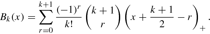 (8.2.19)
 - 6.Summing SVM uses additive kernel function
 (8.2.20)
which is obtained by forming summing kernels, since the sum of two positive definite functions is positive definite.
 :
:

The solution to the problem (8.2.21) was given by Kimeldorf and Wahba in 1971 [24], known as the representer theorem.
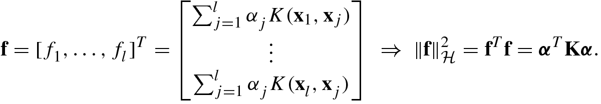
 . Any solution to the optimization problem (8.2.21) for SVMs has a representation of the form

where  .
.
 then we have
 , substituting (8.2.22) into (8.2.21), and using (8.2.23), we get the loss expressed by α:

 it follows that
  , which yields the optimal solution

8.2.3 Semi-Supervised and Graph Regression
Representer theorem for supervised learning (Theorem 8.4) can be extended to semi-supervised learning and/or graph signals.
 , a set of u unlabeled examples
 , and the graph LaplacianL. The minimizer of semi-supervised/graph optimization problem


in terms of the labeled and unlabeled examples.
Note that the above representer theorem [2] is different from the generalized representer theorem in [35]. When the graph Laplacian L = I, Theorem 8.5 reduces to the representer theorem for semi-supervised learning. If letting further u = 0, then Theorem 8.5 reduces to the representer theorem 8.4 for supervised learning.
Theorem 8.5 shows that the optimization problem (8.2.26) is equivalent to finding the optimal solution α ∗.
 and using (8.2.23), then the loss in (8.2.26) can be represented as [2]:

![$$\mathbf {y}=[y_1^{\,} ,\ldots ,y_l^{\,} ,0,\ldots ,0]^T$$](../images/492994_1_En_8_Chapter/492994_1_En_8_Chapter_TeX_IEq91.png) is the (l + u)-dimensional label vector, and J = Diag(1, …, 1, 0, …, 0) is an (l + u) × (l + u) diagonal matrix with the first l diagonal entries 1 and the rest 0.
is the (l + u)-dimensional label vector, and J = Diag(1, …, 1, 0, …, 0) is an (l + u) × (l + u) diagonal matrix with the first l diagonal entries 1 and the rest 0. , one has the first-order optimization condition


 , it is easy to get

8.2.4 Kernel Partial Least Squares Regression
Given two data blocks X and Y, consider kernel methods for partial least squares (PLS) regression. This type of methods is known as the kernel partial least squares regression.
Kernel PLS regression is a natural extension of PLS regression discussed in Sect. 6.9.2.
- 1.
w = X Tu∕(u Tu).
- 2.
t = Xw.
- 3.
c = Y Tt∕(t Tt).
- 4.
u = Y Tc∕(c Tc).
- 5.
p = X Tt∕(t Tt).
- 6.
q = Y Tu∕(u Tu).
- 7.
X = X −tp T.
- 8.
Y = Y −tc T.


- 1.
Randomly initialize u.
- 2.
t = Φ Φ Tu, t ←t∕(t Tt).
- 3.
c = Y Tt.
- 4.
u = Y Tu, u ←u∕(u Tu).
- 5.
Repeat Steps 2–4 until convergence of t.
- 6.
Deflate the matrix: Φ Φ T = (I −tt T) Φ Φ T(I −tt T)T.
- 7.
Deflate the matrix: Y = Y −tc T.
The kernel NIPALS regression is an iterative process: after extraction of the first component t 1 the algorithm starts again using the deflated matrices Φ Φ T and Y computed in Step 6 and Step 7, and repeat Steps 2–7 until the deflated matrix Φ Φ T or Y becomes a null matrix.

 -values can be predicted as

MATLIB code for Kernel RLS algorithm can be found in [28, Appendix III].
8.2.5 Laplacian Support Vector Machines
 and a set of u unlabeled graph examples
  . Let f be a semi-supervised SVM for graph training samples. The graph or Laplacian support vector machines are extended by solving the following optimization problem [2]:


![$$\displaystyle \begin{aligned} L({\boldsymbol \alpha},{\boldsymbol \xi},b,\beta ,\zeta )&=\frac 1l\sum_{i=1}^l \xi_i^{\,} +\frac 12 {\boldsymbol \alpha}^T \left (2\gamma_A^{\,}\mathbf{ K}+2\frac{\gamma_l^{\,}} {(l+u)^2}\mathbf{KLK}\right ){\boldsymbol \alpha}\\ &\quad -\sum_{i=1}^l\beta_i^{\,} \left [y_i^{\,} \left (\sum_{j=1}^{l+u}\alpha_j^{\,} K({\mathbf{x}}_i^{\,} ,{\mathbf{x}}_j^{\,} )+b\right )-1+\xi_i^{\,} \right ]- \sum_{i=1}^l\zeta_i^{\,}\xi_i^{\,} .{} \end{aligned} $$](../images/492994_1_En_8_Chapter/492994_1_En_8_Chapter_TeX_Equ75.png)


 .
.

8.3 Support Vector Machine Regression
The support vector machine regression is a binary regressor algorithm that looks for an optimal hyperplane as a decision function in a high-dimensional space.
8.3.1 Support Vector Machine Regressor
Suppose we are given a training set of N data points  , where
  is the kth input pattern and
  is the kth associated “truth”.
Let  be a mapping from the input space
  to the feature space F. Here, ϕ(x
i) is the extracted feature of the input x
i.
to the feature space F. Here, ϕ(x
i) is the extracted feature of the input x
i.

![$$\displaystyle \begin{aligned} &\text{subject to}~~ \sum_{i=1}^N y_i^{\,} \left [{\mathbf{w}}^T{\boldsymbol \phi}({\mathbf{x}}_i^{\,} )-b\right ]\geq 0, \end{aligned} $$](../images/492994_1_En_8_Chapter/492994_1_En_8_Chapter_TeX_Equ80.png)
![$$\displaystyle \begin{aligned} \gamma =\sum_{i=1}^N y_i^{\,}[\langle \mathbf{w},{\boldsymbol \phi}({\mathbf{x}}_i^{\,} )\rangle -b] \end{aligned} $$](../images/492994_1_En_8_Chapter/492994_1_En_8_Chapter_TeX_Equ81.png)
![$$\displaystyle \begin{aligned} \min_{\mathbf{w},b}\left \{ L(\mathbf{w},b)=\|\mathbf{w}\|{}_2^2 -\sum_{i=1}^N\alpha_i y_i\left [{\mathbf{w}}^T{\boldsymbol \phi}({\mathbf{x}}_i^{\,} )-b\right ]\right\}, \end{aligned} $$](../images/492994_1_En_8_Chapter/492994_1_En_8_Chapter_TeX_Equ82.png)
 are nonnegative.


 .
.
8.3.2 𝜖-Support Vector Regression
The basic idea of 𝜖-support vector (SV) regression is to find a function f(x) = w
Tϕ(x) + b that has at most 𝜖 deviation from the actually obtained targets  for all the training data
  , namely
  for i = 1, …, N, and at the same time w is as flat as possible. In other words, we do not count errors as long as they are less than 𝜖, but will not accept any deviation larger than this [36].
 . Hence, the basic form of 𝜖-support vector regression can be written as a convex optimization problem [36, 43]:


 , for given parameters C > 0 and 𝜖 > 0. Hence we have the standard form of support vector regression given by Vapnik [44]


 is the lower training error subject to 𝜖-insensitive tube
  .
.

 are Lagrange multipliers which have to satisfy the positivity constraints:

 and
and  .
.


 and gives the dual function


![$$\mathbf {Q}=[K({\mathbf {x}}_i^{\,},{\mathbf {x}}_j^{\,})]_{i,j=1}^{N,N}$$](../images/492994_1_En_8_Chapter/492994_1_En_8_Chapter_TeX_IEq117.png) is an N × N positive semi-definite matrix with
is an N × N positive semi-definite matrix with  being the kernel function of SVM.


 , then the inequalities become equalities.
8.3.3 ν-Support Vector Machine Regression


 , while maximizing over the dual variables
  yields


 defined in (8.3.41) leads to the optimization problem called the Wolfe dual. The Wolfe dual ν-support vector machine regression problem can be written as [34]

![$$\displaystyle \begin{aligned} &\text{subject to}~~\sum_{i=1}^N (\alpha_i^{\,}-\alpha_i^* )=0,~~\alpha_i^*\in \left [ 0,\frac CN\right ],~~\sum_{i=1}^N (\alpha_i^{\,}+\alpha_i^* )\leq C\nu . \end{aligned} $$](../images/492994_1_En_8_Chapter/492994_1_En_8_Chapter_TeX_Equ126.png)

ν is an upper bound on the fraction of errors.
ν is a lower bound on the fraction of SVs.

8.4 Support Vector Machine Binary Classification
A basic task in data analysis and pattern recognition is classification that requires the construction of a classifier, namely a function that assigns a class label to instances described by a set of attributes.
In this section we discuss SVM binary classification problems with two classes.
8.4.1 Support Vector Machine Binary Classifier
 , where x
k is the kth input pattern and
, where x
k is the kth input pattern and  is the kth output pattern. Denote the set of data

A SVM classifier is a classifier which finds the hyperplane that separates the data with the largest distance between the hyperplane and the closest data point (called margin).


 , the SVM classifier w is usually designed as


The set of vectors {x 1, …, x N} is said to be optimally separated by the hyperplane if it is separated without error and the distance between the closest vector to the hyperplane is maximal.


 into a higher-dimensional space, but this function is not explicitly constructed.
 in (8.4.10), the margin of a classifier is given by


 is the Lagrange multiplier corresponding to ith training sample
  , and vectors
  satisfying
  are termed support vectors.

- 1.
In order to reduce the likelihood of overfitting the classifier to the training data, the ratio of the number of training examples to the number of features should be at least 10:1. For the same reason the ratio of the number of training examples to the number of unknown parameters should be at least 10:1.
- 2.
Importantly, proper error-estimation methods should be used, especially when selecting parameters for the classifier.
- 3.
Some algorithms require the input features to be scaled to similar ranges, such as some kind of a weighted average of the inputs.
- 4.
There is no single best classification algorithm!
8.4.2 ν-Support Vector Machine Binary Classifier
Similar to ν-SVR, by introducing a new parameter ν ∈ (0, 1] in SVM classification, Schölkopf et al. [34] presented ν-support vector classifier (ν-SVC).


 , and consider the Lagrange function
![$$\displaystyle \begin{aligned} \mathbb{L}(\mathbf{w},{\boldsymbol \xi},b,\rho ,{\boldsymbol \alpha},\beta ,\delta )&=\frac 12\|\mathbf{w}\|{}_2^2-\nu\rho +\frac 1N \sum_{i=1}^N \xi_i^{\,}-\delta\rho \\ &\quad -\sum_{i=1}^N\left (\alpha_i^{\,}\left [y_i^{\,}({\mathbf{w}}^T{\mathbf{x}}_i^{\,}+b)-\rho +\xi_i^{\,}\right ]+ \beta_i^{\,}\xi_i^{\,}\right ).{} \end{aligned} $$](../images/492994_1_En_8_Chapter/492994_1_En_8_Chapter_TeX_Equ154.png)


 , using
  and incorporating the kernel function K(x, x
i) instead of
and incorporating the kernel function K(x, x
i) instead of  in dot product, then one obtains the Wolfe dual optimization problem for ν-SVC as follows:


To compute parameters b and ρ in the primal ν-SVC optimization problem, consider two sets S
+ and S
−, containing support vectors x
i with  and
and  .
.


8.4.3 Least Squares SVM Binary Classifier
Standard SVMs are powerful tools for data classification by assigning them to one of two disjoint halfspaces in either the original input space for linear classifiers, or in a higher-dimensional feature space for nonlinear classifiers. The least squares SVM (LS-SVMs) developed in [37] and the proximal SVMs (PSVMs) presented in [14, 15] are two much simpler classifiers, in which each class of points is assigned to the closest of two parallel planes (in input or feature space) such that they are pushed apart as far as possible.


 .
.![$$\displaystyle \begin{aligned} \mathbb{L}&=\mathbb{L}(\mathbf{w},b,\mathbf{e};{\boldsymbol \alpha})\\ &=\frac 12 \|\mathbf{w}\|{}_2^2+\frac{C}2\sum_{k=1}^N e_k^2-\sum_{k=1}^N \alpha_k \left [y_k^{\,}\left ({\mathbf{w}}^T{\boldsymbol \phi}({\mathbf{x}}_k)+b\right )-1+e_k\right ],{} \end{aligned} $$](../images/492994_1_En_8_Chapter/492994_1_En_8_Chapter_TeX_Equ168.png)


![$$\mathbf {Z}=[y_1^{\,}{\boldsymbol \phi }({\mathbf {x}}_1),\ldots ,y_N^{\,}{\boldsymbol \phi }({\mathbf {x}}_N)]\hskip -0.35mm \in \hskip -0.35mm \mathbb {R}^{m\times N}$$](../images/492994_1_En_8_Chapter/492994_1_En_8_Chapter_TeX_IEq140.png) ,
, ![$$\mathbf {y}=[y_1^{\,},\ldots ,y_N^{\,}]^T\hskip -0.25mm ,$$](../images/492994_1_En_8_Chapter/492994_1_En_8_Chapter_TeX_IEq141.png) 1 = [1, …, 1]T , e = [e
1, …, e
N]T and α = [α
1, …, α
N]T.
1 = [1, …, 1]T , e = [e
1, …, e
N]T and α = [α
1, …, α
N]T.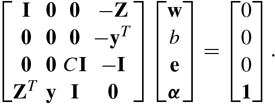
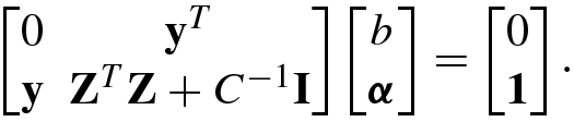
![$$\displaystyle \begin{aligned}{}[{\mathbf{Z}}^T\mathbf{Z}]_{ij}=y_i^{\,}y_j^{\,}{\boldsymbol \phi}^T ({\mathbf{x}}_i){\boldsymbol \phi}({\mathbf{x}}_j)=y_i^{\,}y_j^{\,}K( {\mathbf{x}}_i,{\mathbf{x}}_j). \end{aligned} $$](../images/492994_1_En_8_Chapter/492994_1_En_8_Chapter_TeX_Equ175.png)
 , constant C > 0, and the kernel function K(x
i, x
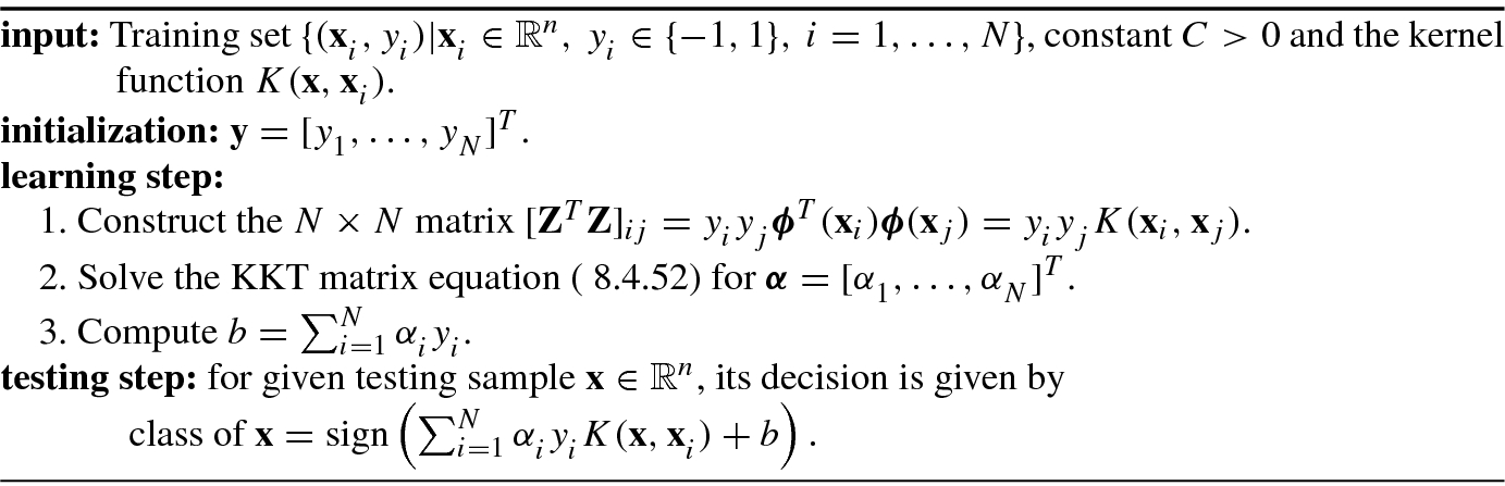
j), the LS-SVM binary classification algorithm performs the following learning step:
, constant C > 0, and the kernel function K(x
i, x
j), the LS-SVM binary classification algorithm performs the following learning step: Construct the N × N matrix
![$$[{\mathbf {Z}}^T\mathbf {Z}]_{ij}=y_i^{\,}y_j^{\,}{\boldsymbol \phi }^T ({\mathbf {x}}_i){\boldsymbol \phi }(\mathbf { x}_j)=y_i^{\,}y_j^{\,}K( {\mathbf {x}}_i,{\mathbf {x}}_j)$$](../images/492994_1_En_8_Chapter/492994_1_En_8_Chapter_TeX_IEq143.png) .
.Solve the KKT matrix equation (8.4.46) for
![$${\boldsymbol \alpha }=[\alpha _1^{\,} ,\ldots ,\alpha _N^{\,} ]^T$$](../images/492994_1_En_8_Chapter/492994_1_En_8_Chapter_TeX_IEq144.png) and b.
and b.
 , its decision is given by

8.4.4 Proximal Support Vector Machine Binary Classifier
Due to the simplicity of their implementations, least square SVM (LS-SVM) and proximal support vector machine (PSVM) have been widely used in binary classification applications.
In the standard SVM binary classifier a plane midway between two parallel bounding planes is used to bound two disjoint halfspaces each of which contains points mostly of class 1 or 2. Similar to the LS-SVM, the key idea of PSVM [14] is that the separation hyperplanes are “proximal” planes rather than bounded planes anymore. Proximal planes classify data points depending on proximity to either one of the two separation planes. We aim to push away proximal planes as far apart as possible. Different from LS-SVM, PSVM uses  instead of
  as the objective function, making the optimization problem strongly convex and has little or no effect on the original optimization problem [22].


By Fung and Mangasarian [15], the PSVM formulation (8.4.49) can be also interpreted as a regularized least squares solution [38] of the system of linear equations  , that is, finding an approximate solution (w, b) to
  with least 2-norm
  .
.

 , and
, and  , and eliminating w and
  , one gets the KKT equation of linear PSVM classifier in matrix form:


![$$\displaystyle \begin{aligned} \mathbf{Z}&=\left [y_1^{\,}{\mathbf{x}}_1^{\,},\ldots ,y_N^{\,}{\mathbf{x}}_N^{\,}\right ],{} \end{aligned} $$](../images/492994_1_En_8_Chapter/492994_1_En_8_Chapter_TeX_Equ182.png)
![$$\displaystyle \begin{aligned} \mathbf{y}&=[y_1^{\,},\ldots ,y_N^{\,}]^T,{} \end{aligned} $$](../images/492994_1_En_8_Chapter/492994_1_En_8_Chapter_TeX_Equ183.png)
![$$\displaystyle \begin{aligned} {\boldsymbol \alpha}&=[\alpha_1^{\,},\ldots ,\alpha_N^{\,}]^T.{}\end{aligned} $$](../images/492994_1_En_8_Chapter/492994_1_En_8_Chapter_TeX_Equ184.png)
Similar to LS-SVM, the training data x can be mapped from the input space  into the feature space ϕ : x →ϕ(x). Hence, the nonlinear PSVM classifier has still the KKT equation (8.4.52) with
 ![$$\mathbf {Z}=[y_1^{\,}{\boldsymbol \phi }({\mathbf {x}}_1^{\,}),\ldots ,y_N^{\,}{\boldsymbol \phi } ({\mathbf {x}}_N^{\,})]$$](../images/492994_1_En_8_Chapter/492994_1_En_8_Chapter_TeX_IEq155.png) in Eq. (8.4.54).
in Eq. (8.4.54).
Algorithm 8.1 shows the PSVM binary classification algorithm.

SVM, LS-SVM, and PSVM are originally proposed for binary classification.
LS-SVM and PSVM provide fast implementations of the traditional SVM. Both LS-SVM and PSVM use equality optimization constraints instead of inequalities from the traditional SVM, which results in a direct least square solution by avoiding quadratic programming.
It should be noted [22] that the Lagrange multipliers  are proportional to the training errors
  in LS-SVM, while in the conventional SVM, many Lagrange multipliers
  are typically equal to zero. As compared to the conventional SVM, sparsity is lost in LS-SVM; this is true to PSVM as well.
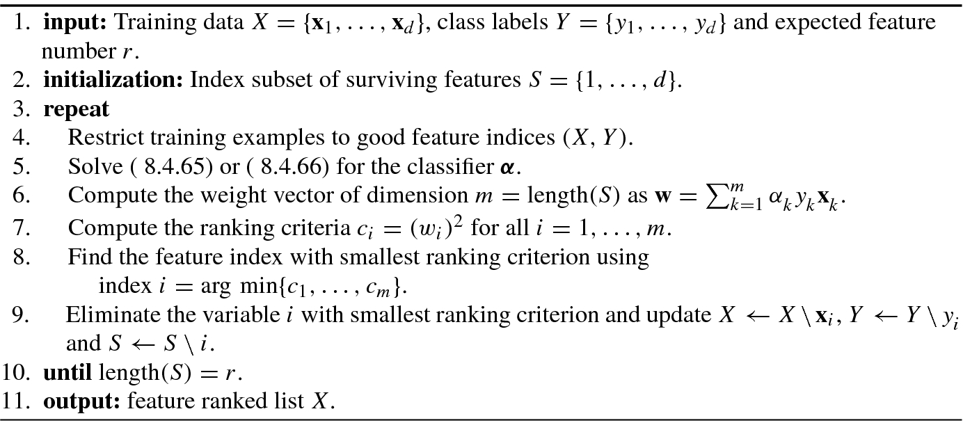
8.4.5 SVM-Recursive Feature Elimination


![$$\displaystyle \begin{aligned} \min_{\mathbf{w},b,{\boldsymbol \alpha}}\Bigg \{L(\mathbf{w},b,{\boldsymbol \alpha})=\frac 12\|\mathbf{w}\|{}_2 -\sum_{i=1}^n\alpha_i[y_i^{\,} ({\mathbf{x}}_i^T\mathbf{ w}+b)-1]\Bigg \}, \end{aligned} $$](../images/492994_1_En_8_Chapter/492994_1_En_8_Chapter_TeX_Equ190.png)


In conclusion, when used for classification, SVMs separate a given set of binary labeled training data (x i, y i) with hyperplane (w, b) that is maximally distant from them. Such a hyperplane is known as “the maximal margin hyperplane.”

 [31]:
[31]:

![$$[{\mathbf {K}}^{(i)}]_{jk}=K_{jk}^{(i)}=\langle {\boldsymbol \phi }({\mathbf {x}}_j^{(i)},{\boldsymbol \phi }({\mathbf {x}}_k^{(i)}\rangle $$](../images/492994_1_En_8_Chapter/492994_1_En_8_Chapter_TeX_IEq160.png) is the (j, k)th entry of the Gram matrix K
(i)of the training data when variable i is removed, and
is the (j, k)th entry of the Gram matrix K
(i)of the training data when variable i is removed, and  is the corresponding solution of (8.4.66). For the sake of simplicity,
  is usually taken even if a variable has been removed in order to reduce the computational complexity of the SVM-RFE algorithm.
Algorithm 8.2 shows the SVM-RFE algorithm that is an application of RFE using the weight magnitude as ranking criterion.
8.5 Support Vector Machine Multiclass Classification
A multiclass classifier is a function  that maps an instance
  into an element y of
  .
.
8.5.1 Decomposition Methods for Multiclass Classification
A popular way to solve a k-class problem is to decompose it to a set of L binary classification problems. One-versus-one, one-versus-rest, and directed acyclic graph SVM methods are three of the most common decomposition approaches [21, 41, 48].
The standard method for k-class SVM classification is to construct L = k binary classifiers  . The ith SVM will be trained with all of the examples in the ith class with positive labels, and all other examples with negative labels. Then, the weight vector w
m for the mth model can be generated by any linear classifier. Such an SVM classification method is referred to as one-against-all (OAA) or one-versus-rest (OVR) method [4, 27].
. The ith SVM will be trained with all of the examples in the ith class with positive labels, and all other examples with negative labels. Then, the weight vector w
m for the mth model can be generated by any linear classifier. Such an SVM classification method is referred to as one-against-all (OAA) or one-versus-rest (OVR) method [4, 27].
Let  be a set of N training examples, and each example
  be drawn from a domain
  and
and  is the class of
  .
.


![$${\mathbf {w}}_m^{\,}=[w_{m,1},\cdots ,w_{m,n}]^T,\,m=1,\ldots ,k$$](../images/492994_1_En_8_Chapter/492994_1_En_8_Chapter_TeX_IEq172.png) is the weight vector of the mth classifier, C is the penalty parameter, and
is the weight vector of the mth classifier, C is the penalty parameter, and  is the training error corresponding to the mth class and the ith training data
  that is mapped to a higher-dimensional space by the function
  .
.Minimizing  means maximizing the margin
  between two groups of data. When data are not linear separable, there is a penalty term
  which can reduce the training errors in the mth classifier. The basic concept behind one-against-all SVM is to search for a balance between the regularization term
  and the training error
  for the m classifiers.
By “decision function” it means a function f(x) whose sign represents the class assigned to data point x.
 . Hence, a new testing instance x is said to be in the class which has the largest value among k decision functions:

The one-against-one (OAO) method [13, 25] is also known as one-versus-one (OVO) method. This method constructs L = k(k − 1)∕2 binary classifiers by solving k(k − 1)∕2 binary classification problems [25]. Each binary classifier constructs a model with data from one class as positive and another class as negative. Since there is k(k − 1)∕2 combinations of two classes, one needs to construct k(k − 1)∕2 weight vectors: w 1,2, …, w 1,k;w 2,3, …, w 2,k;…;w k−1,k.


After all k(k − 1)∕2 binary classifiers are constructed by solving the above binary problems for i, j = 1, …, k, the following voting strategy suggested in [25] can be used: if the decision function sign((w ij)Tϕ(x) + b ij) determines that x is in ith class, then vote for the ith class is added by one. Otherwise, the vote for jth is added by one. Finally, x is predicted to be in the class with the largest vote. This voting approach is also called the “Max Wins” strategy. In case that two classes have identical votes, thought it may not be a good strategy, we simply select the one with the smaller index [21].
Directed acyclic graph SVM method [27] is simply called DAGSVM method whose training phase is the same as the one-against-one method by solving binary SVMs. However, in the testing phase, it uses a rooted binary directed acyclic graph which has internal nodes and leaves.
The training phase of the DAGSVM method is the same as the one-against-one method by solving k(k − 1)∕2 binary SVM classification problems, but uses one different voting strategy, called a rooted binary directed acyclic graph which has k(k − 1)∕2 internal nodes and k leaves, in the testing phase. Each node is a binary SVM classifier of ith and jth classes.
A directed acyclic graph (DAG) is a graph whose edges have an orientation and no cycles.
Given a space X and a set of Boolean functions  , the decision directed acyclic graphs (DDAGs) on k classes over
  are functions which can be implemented using a rooted binary DAG with k leaves labeled by the classes where each of the L = k(k − 1)∕2 internal nodes is labeled with an element of
  . The nodes are arranged in a triangle with the single root node at the top, two nodes in the second layer, and so on until the final layer of k leaves. The ith node in layer j < k is connected to the ith and (i + 1)th node in the (j + 1)st layer.
For k-class classification, a rooted binary directed acyclic graph has k layers: the top layer has a single root node, the second layer has two nodes, and so on until the kth (i.e., final) layer has k nodes, so a rooted binary DAG has k leaves and 1 + 2 + ⋯ + k = k(k − 1)∕2 internal nodes. Each node is a binary SVM of ith and jth classes.
The DDAG is equivalent to operating on a list, where each node eliminates one class from the list. The list is initialized with a list of all classes. A test point is evaluated against the decision node that corresponds to the first and last elements of the list. If the node prefers one of the two classes, the other class is eliminated from the list, and the DDAG proceeds to test the first and last elements of the new list. The DDAG terminates when only one class remains in the list. Thus, for a problem with k classes, k − 1 decision nodes will be evaluated in order to derive an answer.
Given N test samples  with
with  and
and  3, 4}. The DDAG is equivalent to operating on a list {1, 2, 3, 4}, where each node eliminates one class from the list. The list is starting at the root node 1 versus 4 at the top layer, the binary decision function is evaluated. If the output value is not Class 1, then it is eliminated from the list to get a new list {2, 3, 4} and thus we make the binary decision of two classes 2 versus 4. If the root node prefers Class 1, then Class 4 at the root node is removed from the list to yield a new list {1, 2, 3} and the binary decision is made for two classes 1 versus 3. Then, the second layer has two nodes (2 vs 4) and (1 vs 3). Therefore, we go through a path until DDAG terminates when only one class remains in the list.
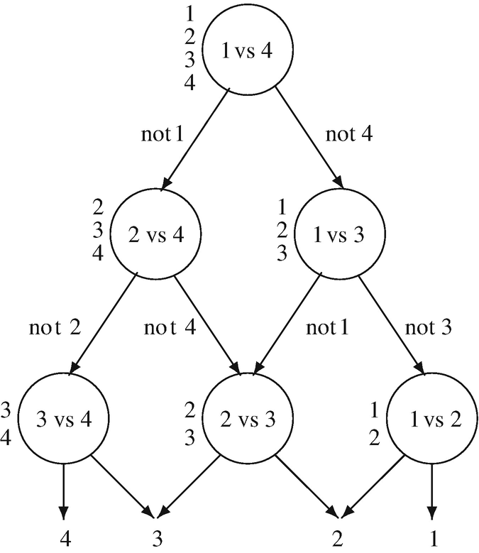
The decision directed acyclic graphs (DDAG) for finding the best class out of four classes
DDAGs naturally generalize the class of Decision Trees, allowing for a more efficient representation of redundancies and repetitions that can occur in different branches of the tree, by allowing the merging of different decision paths [27].
8.5.2 Least Squares SVM Multiclass Classifier
The previous subsection discussed the support vector machine binary classifier. In this subsection we discuss multi-class classification cases.
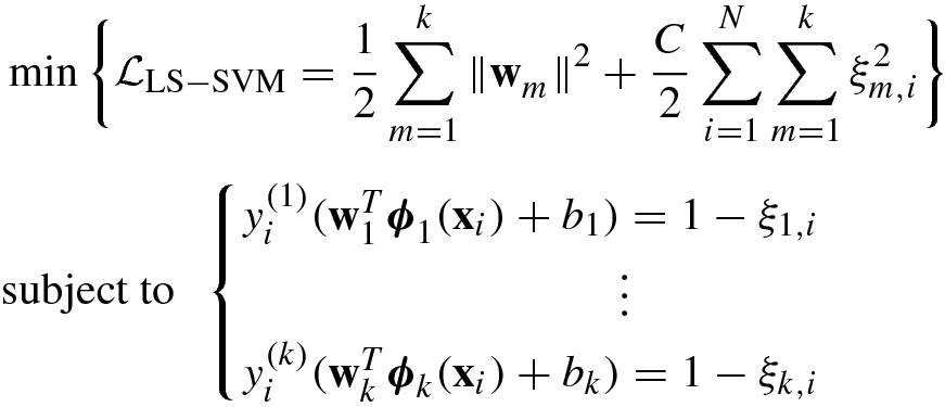

![$$\displaystyle \begin{aligned} &\quad -\sum_{i=1}^N\sum_{m=1}^k \alpha_{m,i}\left [y_i^{\,}\left ({\mathbf{w}}_m^T{\boldsymbol \phi}_m^{\,}({\mathbf{x}}_i)+b_m^{\,} \right )-1+\xi_{m,i}^{\,}\right ] \end{aligned} $$](../images/492994_1_En_8_Chapter/492994_1_En_8_Chapter_TeX_Equ205.png)


![$$\displaystyle \begin{aligned} {\mathbf{Z}}_m^{\,} &=[y_1^{(m)}{\boldsymbol \phi}_m^{\,} ({\mathbf{x}}_1^{\,} ),\ldots ,y_N^{(m)}{\boldsymbol \phi}_m^{\,} ({\mathbf{x}}_N^{\,} )],{} \end{aligned} $$](../images/492994_1_En_8_Chapter/492994_1_En_8_Chapter_TeX_Equ210.png)
![$$\displaystyle \begin{aligned} {\mathbf{w}}_m^{\,} &=[w_{m,1}^{\,} ,\ldots ,w_{m,N}^{\,}]^T, \end{aligned} $$](../images/492994_1_En_8_Chapter/492994_1_En_8_Chapter_TeX_Equ211.png)
![$$\displaystyle \begin{aligned} {\mathbf{y}}^{(m)}&=[y_1^{(m)},\ldots ,y_N^{(m)}]^T, \end{aligned} $$](../images/492994_1_En_8_Chapter/492994_1_En_8_Chapter_TeX_Equ212.png)
![$$\displaystyle \begin{aligned} {\boldsymbol \alpha}_m^{\,} &=[\alpha_{m,1}^{\,},\ldots ,\alpha_{m,N}]^T, \end{aligned} $$](../images/492994_1_En_8_Chapter/492994_1_En_8_Chapter_TeX_Equ213.png)
![$$\displaystyle \begin{aligned} {\boldsymbol \xi}_m^{\,} &=[\xi_{m,1}^{\,} ,\ldots ,\xi_{m,N}^{\,} ]^T.{} \end{aligned} $$](../images/492994_1_En_8_Chapter/492994_1_En_8_Chapter_TeX_Equ214.png)
 , one has

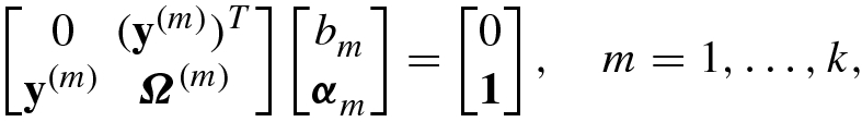
 with the (i, j)th entries

 (if i = j) or 0 (otherwise); and
  is the kernel function of the mth SVM for multiclass classification.
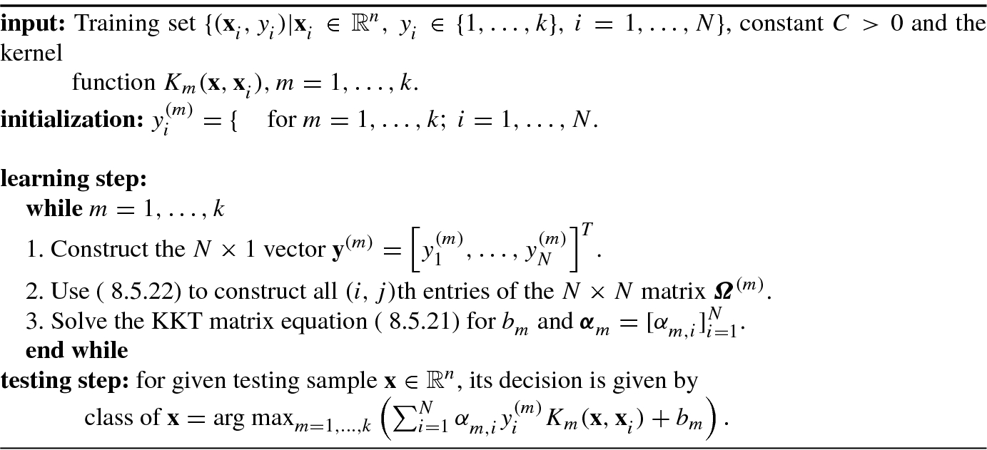
Algorithm 8.3 shows the LS-SVM multiclass classification algorithm.
8.5.3 Proximal Support Vector Machine Multiclass Classifier


 and
and  in the above equations yields the KKT equations


![$$\displaystyle \begin{aligned} {\mathbf{Z}}_m&=\left [y_1^{(m)}{\boldsymbol \phi}_m^{\,} ({\mathbf{x}}_1^{\,} ),\ldots ,y_N^{(m)}{\boldsymbol \phi}_m^{\,} ({\mathbf{x}}_N^{\,} ) \right ],{} \end{aligned} $$](../images/492994_1_En_8_Chapter/492994_1_En_8_Chapter_TeX_Equ227.png)
![$$\displaystyle \begin{aligned} {\mathbf{y}}_m^{\,} &=[y_1^{(m)},\ldots ,y_N^{(m)}]^T,{} \end{aligned} $$](../images/492994_1_En_8_Chapter/492994_1_En_8_Chapter_TeX_Equ228.png)
![$$\displaystyle \begin{aligned} {\boldsymbol \alpha}_m^{\,} &=[\alpha_{m,1}^{\,} ,\ldots ,\alpha_{m,N}^{\,} ]^T.{} \end{aligned} $$](../images/492994_1_En_8_Chapter/492994_1_En_8_Chapter_TeX_Equ229.png)
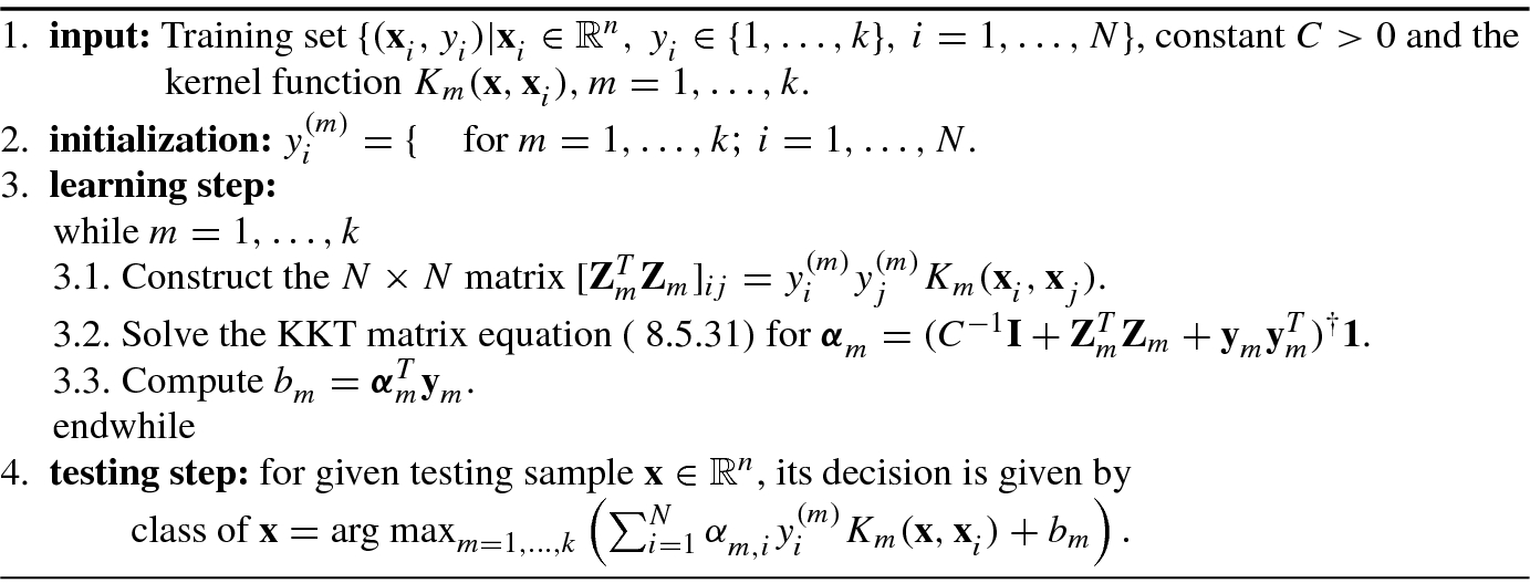
Algorithm 8.4 shows the PSVM multiclass classification algorithm.
8.6 Gaussian Process for Regression and Classification
In Chap. 6 we discussed traditionally parametric models based machine learning. The parametric models have a possible advantage in ease of interpretability, but for complex data sets, simple parametric models may lack expressive power, and their more complex counterparts (such as feedforward neural networks) may not be easy to work with in practice [29, 30]. The advent of kernel machines, such as Gaussian processes, sparse Bayesian learning, and relevance vector machine, has opened the possibility of flexible models which are practical to work with.
In this section we deal with Gaussian process methods for regression and classification problems.
8.6.1 Joint, Marginal, and Conditional Probabilities
 and
and  , where A ∪ B = {1, …, n} and A ∩ B = ∅, so that
  . Each group may contain one or more variables. The marginal probability of
  , denoted by
  , is given by marginal probability


 , as it is not meaningful to condition on an impossible event. If
  and
and  are independent, then the marginal
  and the conditional
  are equal.
 and
and  we obtain Bayes theorem

8.6.2 Gaussian Process
A random variable x with the normal distribution  is called the univariate Gaussian distribution, and is denoted as x ∼ N(μ, σ
2), where μ = E{x} and σ
2 = var(x) are its mean and variance, respectively.
is called the univariate Gaussian distribution, and is denoted as x ∼ N(μ, σ
2), where μ = E{x} and σ
2 = var(x) are its mean and variance, respectively.

![$${\boldsymbol \mu }=[\mu _1,\ldots ,\mu _N^{\,} ]^T$$](../images/492994_1_En_8_Chapter/492994_1_En_8_Chapter_TeX_IEq207.png) with μ
i = E{x
i} is the mean vector (of length N) of x and Σ is the N × N (symmetric, positive definite) covariance matrix of x. The multivariate Gaussian distribution is denoted simply as x ∼ N(μ, Σ).
with μ
i = E{x
i} is the mean vector (of length N) of x and Σ is the N × N (symmetric, positive definite) covariance matrix of x. The multivariate Gaussian distribution is denoted simply as x ∼ N(μ, Σ).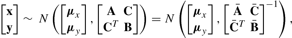


A Gaussian process is a natural generalization of multivariate Gaussian distribution.
A Gaussian Process f(x) is a collection of random variables x, any finite number of which have (consistent) joint Gaussian distributions.
Clearly, the Gaussian distribution is over vectors, whereas the Gaussian process is over functions f(x), where x is a Gaussian vector.


The covariance function K(x
i, x
j) (also known as kernel, kernel function, or covariance kernel) is the driving factor in Gaussian processes for regression and/or classification. Actually, the kernel represents the particular structure present in the data  being modeled. One of the main difficulties in applying Gaussian processes is to construct such a kernel.

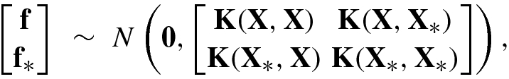
8.6.3 Gaussian Process Regression
Let {(x n, f n)| n = 1, …, N} be the training samples, where f n, n = 1, …, N are the noise-free training outputs of x n, typically continuous functions for regression or discrete function for classification.
![$$\mathbf {f}=[f_1^{\,} ,\ldots ,f_N^{\,} ]^T$$](../images/492994_1_En_8_Chapter/492994_1_En_8_Chapter_TeX_IEq209.png) and the test output vector
and the test output vector ![$${\mathbf {f}}_*=[f_1^*,\ldots , f_{N_*}^*]^T$$](../images/492994_1_En_8_Chapter/492994_1_En_8_Chapter_TeX_IEq210.png) given the test samples
given the test samples  . Under the assumption of Gaussian distributions f ∼ N(0, K(X, X)) and f
∗ ∼ N(0, K(X
∗, X
∗)), the joint distribution of f and f
∗ is given by
. Under the assumption of Gaussian distributions f ∼ N(0, K(X, X)) and f
∗ ∼ N(0, K(X
∗, X
∗)), the joint distribution of f and f
∗ is given by
![$$\mathbf {X}=[{\mathbf {x}}_1^{\,} ,\ldots ,{\mathbf {x}}_N^{\,} ]$$](../images/492994_1_En_8_Chapter/492994_1_En_8_Chapter_TeX_IEq212.png) and
and ![$${\mathbf {X}}_*=[{\mathbf {x}}_1^*,\ldots ,{\mathbf {x}}_{N_*}^*]$$](../images/492994_1_En_8_Chapter/492994_1_En_8_Chapter_TeX_IEq213.png) are the N × N training sample matrix and the N
∗× N
∗ test sample matrix, respectively; and
are the N × N training sample matrix and the N
∗× N
∗ test sample matrix, respectively; and  ,
,  ,
,  , and
, and  are the covariance function matrices, respectively.
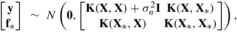
 . In this case, y ∼ N(0, cov(y)) with


![$$\displaystyle \begin{aligned} \bar{\mathbf{f}}_*&=E\{{\mathbf{f}}_*|\mathbf{y}\}=\mathbf{K}({\mathbf{X}}_*,\mathbf{X})\big [\mathbf{K}(\mathbf{X},\mathbf{X})+\sigma_n^2\mathbf{I}\big ]^{-1}\mathbf{ y},{} \end{aligned} $$](../images/492994_1_En_8_Chapter/492994_1_En_8_Chapter_TeX_Equ247.png)
![$$\displaystyle \begin{aligned} \mathrm{cov}({\mathbf{f}}_*)&=\mathbf{K}({\mathbf{X}}_*,{\mathbf{X}}_*)-\mathbf{K}({\mathbf{X}}_*,\mathbf{X})\big [\mathbf{K}(\mathbf{X},\mathbf{X})+\sigma_n^2\mathbf{ I}\big ]^{-1} \mathbf{K}(\mathbf{X},{\mathbf{X}}_*).{} \end{aligned} $$](../images/492994_1_En_8_Chapter/492994_1_En_8_Chapter_TeX_Equ248.png)
 is the mean vector over N
∗ test points, i.e.,
is the mean vector over N
∗ test points, i.e.,  .
. in X. In this case, Eqs. (8.6.18) and (8.6.19) reduce to


 , then the mean vector centered on a test point x
∗, denoted by
, then the mean vector centered on a test point x
∗, denoted by  , is given by

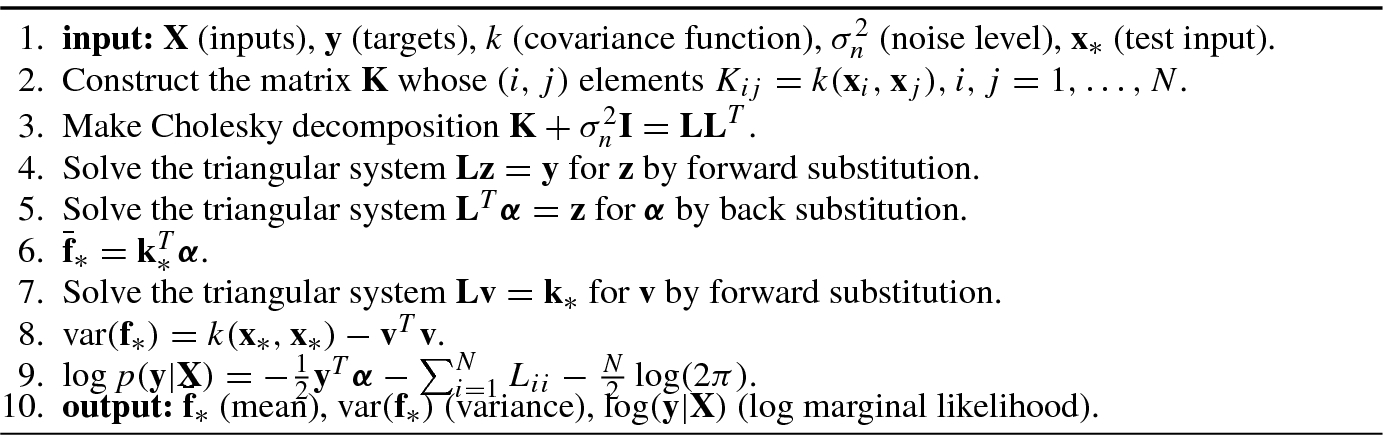
When using Eqs. (8.6.20) and (8.6.21) to compute directly  and var(f
∗), it needs to invert the matrix
and var(f
∗), it needs to invert the matrix  . A faster and numerically more stable computation method is to use Cholesky decomposition.
 be given by
  , where L is a lower triangular matrix. Then,
  becomes α = (L
T)−1L
−1y. Denoting z = L
−1y and α = (L
T)−1z, then
becomes α = (L
T)−1L
−1y. Denoting z = L
−1y and α = (L
T)−1z, then


- 1.
Make Cholesky decomposition:
 .
. - 2.
Solve the triangular system Lz = y for z by forward substitution.
- 3.
Solve the triangular system L Tα = z for α by back substitution.
Similarly, we have  , where v = L
−1k
∗⇔Lv = k
∗. This implies v is the solution for the triangular system Lv = k
∗.
, where v = L
−1k
∗⇔Lv = k
∗. This implies v is the solution for the triangular system Lv = k
∗.
Once α and v are found, one can use Eqs. (8.6.20) and (8.6.21) to get  and var(f
∗) = k(x
∗, x
∗) −v
Tv, respectively.
and var(f
∗) = k(x
∗, x
∗) −v
Tv, respectively.


 , the marginal likelihood
![$$\displaystyle \begin{aligned} \log p(\mathbf{y}|\mathbf{X})=-\frac 12{\mathbf{y}}^T\big [\mathbf{K}+\sigma_n^2\mathbf{I}\big ]^{-1}\mathbf{y}-\frac 12 \log \big |\mathbf{K}+\sigma_n^2\mathbf{ I}\big | -\frac N2 \log (2\pi ). \end{aligned} $$](../images/492994_1_En_8_Chapter/492994_1_En_8_Chapter_TeX_Equ256.png)
 is the model complexity depending only on the covariance function and the inputs. The last term
  is just a normalization constant.
Algorithm 8.5 shows the Gaussian process regression (GPR) in [30].
8.6.4 Gaussian Process Classification
Both regression and classification can be viewed as function approximation problems, but their solutions are rather different. This is because the targets in regression are continuous functions in which the likelihood function is Gaussian; a Gaussian process prior combined with a Gaussian likelihood gives rise to a posterior Gaussian process over functions, and everything remains analytically tractable [30]. But, in classification models, the targets are discrete class labels, so the Gaussian likelihood is no longer appropriate. Hence, approximate inference is only available for classification, where exact inference is not feasible.
- 1.Computing the distribution of the latent variable corresponding to a test case:
 (8.6.28)
where p(f|X, y) = p(y|f)p(f|X)∕p(y|X) is the posterior over the latent variables.
- 2.Using this distribution over the latent f ∗ to produce a probabilistic prediction
 (8.6.29)
In classification due to discrete class labels the posterior p(f|X, y) in (8.6.28) is non-Gaussian, which makes the likelihood in (8.6.28) is non-Gaussian, which makes its integral analytically intractable. Similarly, Eq. (8.6.29) can be intractable analytically for certain sigmoid functions.

 , and
, and  is the Hessian matrix of the negative log posterior at that point.


Gaussian processes are a main mathematical tool for sparse Bayesian learning and hence the relevance vector machine that will be discussed in the next section.
8.7 Relevance Vector Machine
In real-world data, the presence of noise (in regression) and class overlap (in classification) implies that the principal modeling challenge is to avoid “overfitting” of the training set. In order to avoid the overfitting of SVMs (because of too many support vectors), Tipping [39] proposed a relevant vectors based learning machine, called the relevance vector machine (RVM). “Sparse Bayesian learning” is the basis for the RVM.
8.7.1 Sparse Bayesian Regression
 , where the “target” samples
  are conventionally considered to be realizations of a deterministic function y that is corrupted by some additive noise process
  . This function f is usually modeled by a linearly weighted sum of M fixed basis functions
  :
:

 such that
  is a “good” approximation of y(x).
The function approximation has two important benefits: accuracy and “sparsity.” By sparsity, it means that a sparse learning algorithm can set significant numbers of the parameters  to zero.

 is a kernel function, effectively defining one basis function for each example in the training set.
This can avoid overfitting, which leads to good generalization.
This furthermore results in a sparse model dependent only on a subset of kernel functions.
- 1.
Although relatively sparse, SVMs make unnecessarily liberal use of basis functions since the number of support vectors required typically grows linearly with the size of the training set. In order to reduce computational complexity, some form of post-processing is often required.
- 2.
Predictions are not probabilistic. The SVM outputs a point estimate in regression, and a “hard” binary decision in classification. Ideally, it is desired to estimate the conditional distribution p(t|x) in order to capture uncertainty in prediction. Although posterior probability estimates can be coerced from SVMs via post-processing, these estimates are unreliable.
- 3.
Owing to satisfying Mercer’s condition, the kernel function K(x;x i) must be the continuous symmetric kernel of a positive integral operator.

The key feature of this learning approach is that in order to offer good generalization performance, the inferred predictors are exceedingly sparse in that they contain relatively few nonzero w i parameters. Since the majority of parameters are automatically set to zero during the learning process, this learning approach is known as the sparse Bayesian learning for regression [39].
The following are the framework of sparse Bayesian learning for regression.
 , where
  . It is usually assumed that the target values are samples from the model with additive noise 𝜖
n. Under this assumption, the standard linear regression model with additive Gaussian noise is given by
. It is usually assumed that the target values are samples from the model with additive noise 𝜖
n. Under this assumption, the standard linear regression model with additive Gaussian noise is given by

![$$\mathbf {t}=[t_1^{\,} ,\ldots ,t_N^{\,} ]^T$$](../images/492994_1_En_8_Chapter/492994_1_En_8_Chapter_TeX_IEq247.png) be the target vector and
be the target vector and ![$$\mathbf {y}=[y_1^{\,} , \ldots ,y_N^{\,} ]^T$$](../images/492994_1_En_8_Chapter/492994_1_En_8_Chapter_TeX_IEq248.png) be the approximation vector, then under the assumption of independence of the target vector t and the Gaussian noise e = t −y, the likelihood of the complete data set can be written as
be the approximation vector, then under the assumption of independence of the target vector t and the Gaussian noise e = t −y, the likelihood of the complete data set can be written as

- The linear neural network makes predictions based on the function
 (8.7.6)where
![$$\mathbf {w}=[w_1^{\,} ,\ldots ,w_N^{\,} ]^T$$](../images/492994_1_En_8_Chapter/492994_1_En_8_Chapter_TeX_IEq249.png) is the weight vector,
is the weight vector, ![$$\mathbf {X}=[{\mathbf {x}}_1^{\,} ,\ldots ,{\mathbf {x}}_N^{\,} ]$$](../images/492994_1_En_8_Chapter/492994_1_En_8_Chapter_TeX_IEq250.png) is the data matrix, and thus the likelihood (because of the independence assumption) is given by
is the data matrix, and thus the likelihood (because of the independence assumption) is given by
 (8.7.7)
 - The SVM makes predictionswhere
 (8.7.8)
![$$\mathbf {K}=[\mathbf {k}({\mathbf {x}}_1)^{\,} ,\ldots ,\mathbf {k}({\mathbf {x}}_N^{\,} )]^T$$](../images/492994_1_En_8_Chapter/492994_1_En_8_Chapter_TeX_IEq251.png) is the N × (N + 1) kernel matrix with
is the N × (N + 1) kernel matrix with ![$$\mathbf {k}(\mathbf { x}_n)= [1,K({\mathbf {x}}_n,{\mathbf {x}}_1),\ldots ,K({\mathbf {x}}_n^{\,} ,{\mathbf {x}}_N^{\,} )]^T$$](../images/492994_1_En_8_Chapter/492994_1_En_8_Chapter_TeX_IEq252.png) , and
, and ![$$\mathbf {w}=[w_0^{\,} ,w_1^{\,} ,\ldots ,w_N^{\,} ]^T$$](../images/492994_1_En_8_Chapter/492994_1_En_8_Chapter_TeX_IEq253.png) . So under the independence assumption, the likelihood is given by
. So under the independence assumption, the likelihood is given by
 (8.7.9)
 - The RVM makes predictionswhere
 (8.7.10)
![$${\boldsymbol \Phi }=[{\boldsymbol \phi }({\mathbf {x}}_1^{\,} ),\ldots ,{\boldsymbol \phi }({\mathbf {x}}_N^{\,} )]^T$$](../images/492994_1_En_8_Chapter/492994_1_En_8_Chapter_TeX_IEq254.png) is the N × (N + 1) “design” matrix with
is the N × (N + 1) “design” matrix with ![$${\boldsymbol \phi }({\mathbf {x}}_n) =[1,\phi _1({\mathbf {x}}_n),\ldots ,\phi _N^{\,} ({\mathbf {x}}_n)]^T$$](../images/492994_1_En_8_Chapter/492994_1_En_8_Chapter_TeX_IEq255.png) , and
, and ![$$\mathbf {w}=[w_0^{\,} ,w_1^{\,} ,\ldots ,w_N^{\,} ]^T$$](../images/492994_1_En_8_Chapter/492994_1_En_8_Chapter_TeX_IEq256.png) . For example, ϕ(x
n) = [1,
. For example, ϕ(x
n) = [1, ![$$K({\mathbf {x}}_n,{\mathbf {x}}_1),K({\mathbf {x}}_n,{\mathbf {x}}_2),\ldots ,K({\mathbf {x}}_n,{\mathbf {x}}_N^{\,} )]^T$$](../images/492994_1_En_8_Chapter/492994_1_En_8_Chapter_TeX_IEq257.png) . Therefore, the likelihood (because of the independence assumption) is given by
. Therefore, the likelihood (because of the independence assumption) is given by
 (8.7.11)


The Bayesian learning problem, in the context of the RVM, thus becomes the search for the hyperparameters α. In the RVM, these hyperparameters are estimated from minimizing  . This estimation problem will be discussed in Sect. 8.7.3.

![$${\boldsymbol \Phi }=[{\mathbf {r}}_1^{\,} ,\ldots ,{\mathbf {r}}_K^{\,} ]$$](../images/492994_1_En_8_Chapter/492994_1_En_8_Chapter_TeX_IEq259.png) is a K × N matrix, assuming random CS measurements are made.
is a K × N matrix, assuming random CS measurements are made.


8.7.2 Sparse Bayesian Classification
Sparse Bayesian classification follows an essentially identical framework for regression above, but using a Bernoulli likelihood and a sigmoidal link function to account for the change in the target quantities [39].


In sparse Bayesian regression, the weights w can be integrated out analytically. Unlike the regression case, sparse Bayesian classification cannot be integrated out analytically, precluding closed form expressions for either the weight posterior p(w|t, α) or the marginal likelihood P(t|α). Thus, it utilizes the Laplace approximation procedure.
In the statistics and machine leaning literature, the Laplace approximation refers to the evaluation of the marginal likelihood or free energy using Laplace’s method. This is equivalent to a local Gaussian approximation of P(t|w) around a maximum a posteriori (MAP) estimate [40].
8.7.3 Fast Marginal Likelihood Maximization
 on a single hyperparameter α
m, m ∈{1, …, M}, the matrix C in the Eq. (8.7.16) can be decomposed as
on a single hyperparameter α
m, m ∈{1, …, M}, the matrix C in the Eq. (8.7.16) can be decomposed as

 can be written as


 can be rewritten as


 we have the result

 has a unique maximum with respect to α
m [10]:
has a unique maximum with respect to α
m [10]:

If ϕ m is “in the model” (i.e., α m < ∞) yet
 , then ϕ
m may be deleted (i.e., α
m set to ∞).
, then ϕ
m may be deleted (i.e., α
m set to ∞).If ϕ m is excluded from the model (α m = ∞) and
 , then ϕ
m may be added (i.e., α
m is set to some optimal finite value).
, then ϕ
m may be added (i.e., α
m is set to some optimal finite value).
 , it is easier to maintain and compute value of C
−1. Let
, it is easier to maintain and compute value of C
−1. Let

 , postmultiplying ϕ
m, and using (8.7.29), Eq. (8.7.27) yields
, postmultiplying ϕ
m, and using (8.7.29), Eq. (8.7.27) yields


- 1.
Initialize σ 2 to some sensible value (e.g., var[t] × 0.1).
- 2.
All other α m are notionally set to infinity.
- 3.
Explicitly compute Σ and μ (which are scalars initially), along with initial values of s m and q m for all M bases ϕ m.
- 4.
Select a candidate basis vector ϕ i from the set of all M.
- 5.
Compute
 .
. - 6.If θ i > 0 and α i < ∞ (i.e., ϕ i is in the model), re-estimate α i. Defining
 and Σ
j as the jth column of Σ:
and Σ
j as the jth column of Σ:
 (8.7.42)
 (8.7.43)
 (8.7.44)
 (8.7.45)
 (8.7.46)
 - 7.If θ i > 0 and α i = ∞, add ϕ i to the model with updated α i:
 (8.7.47)
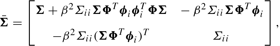 (8.7.48)
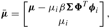 (8.7.49)
 (8.7.50)
 (8.7.51)
where Σ ii = (α i + S i)−1, μ i = Σ iiQ i, and e i = ϕ i − β Φ Σ Φ Tϕ i.
- 8.If θ i ≤ 0 and α i < ∞, then delete ϕ i from the model and set α i = ∞:
 (8.7.52)
 (8.7.53)
 (8.7.54)
 (8.7.55)
 (8.7.56)
Following updates (8.7.53) and (8.7.54), the appropriate row and/or column j is removed from
 and
and  .
. - 9.
If it is a regression model and estimating the noise level, update
 .
. - 10.
Recompute/update Σ, μ (using the Laplace approximation procedure in classification) and all s m and q m using Eqs. (8.7.35)–(8.7.40).
- 11.
If converged terminate, otherwise goto 4.

SVMs have high classification accuracy due to introducing maximum interval.
When the sample size is small, SVMs can also classify accurately and have good generalization ability.
The kernel function can be used to solve nonlinear problems.
SVMs can solve the problem of classification and regression with high-dimensional features.