9
Failures, Real and Imagined
Beginning with the election campaign of 1984, opposition to the Reagan policies centered on the large and growing federal budget deficit. Walter Mondale, Democratic presidential candidate, argued that the deficit was so dangerous that it would be essential to raise taxes in order to reduce it. He made his honesty in promising to raise taxes a major campaign issue, in contrast to President Reagan’s alleged dishonesty in not admitting that he would raise taxes.1 With Reagan insisting that he would cut spending rather than raise taxes, and also that the United States could “grow out of” the deficit, Mondale suffered one of the worst defeats in history, carrying only the District of Columbia and his home state of Minnesota. In 1988, the Democrats continued to harp on the deficit. Vice presidential candidate Lloyd Bentsen was asked how he could criticize the Reagan-Bush administration’s economic policies in the light of the long period of prosperity the nation had enjoyed since the end of the 1981–82 recession. His response was, “If you let me write billions of dollars of hot checks I’ll give you an illusion of prosperity, also.” Again, the public wouldn’t buy the argument. George Bush was elected president in large part because he claimed he could control the deficit by imposing a “flexible freeze” on government spending without raising taxes.
Meanwhile, academic economists were hard at work attempting to warn of the dire long-run consequences of deficits and growing federal debt. Make no mistake about it, there was something different about the deficits experienced as a result of the Volcker-Reagan program. The Council of Economic Advisers noted that difference in early 1985.
Federal borrowing as a share of GNP varied within a narrow range, except during World War II and recessions until the past several years [1981–84]. The ratio of the outstanding debt to GNP increased sharply during the Great Depression and World War II, declined substantially through the 1970s, and has since increased sharply.2
The Alleged Burden of the National Debt
As mentioned in chapter 2, the absolute size of the national debt is probably meaningless when it comes to assessing its impact on the economy. What is important is the ratio of the outstanding debt to the GDP. The reason is clear. Whether one focuses only on the need to spend government revenue paying interest or whether one believes that ultimately future taxpayers will have to “pay off” the debt, the size of the GDP will determine the ability to make those payments. When H. Ross Perot warned in United We Stand that by the year 2000 we might have an $8 trillion national debt, he neglected to mention that by the year 2000 we would have a much larger GDP. In fiscal 1995, the national debt held by the public was about 50 percent of the GDP.3 If GDP grows faster than the national debt between now and the year 2000, that $8 trillion national debt would be a smaller percentage of GDP. American taxpayers, thus, would pay a smaller percentage of their tax dollars toward interest on the debt than they do now.
Also despite the quadrupling of the national debt during the 1980s, interest payments remain a relatively small percentage of GDP and have not gone beyond 14 percent of the entire federal budget.4
It is true that over the period from 1979 to 1989, interest payments as a percentage of the federal budget almost doubled. This trend and the rising interest payments as a percentage of GDP cannot, of course, go on indefinitely. However, to suggest that the absolute level that has been reached as a percentage of GDP is unsustainable in just not true.
The other often-quoted part of the argument is the assertion that “our children” or “our grandchildren” will have to “pay off” the national debt with a crushing tax burden. Some economists talk of debt-financed government spending as an intergenerational transfer of wealth. The current generation borrows, and the future generation pays for it. This is total nonsense, and a moment’s reflection should demonstrate that point conclusively. Individuals have to pay off debts because lending institutions know that sooner or later they will die, and if they die without sufficient assets to cover their unpaid debts, the lender will be stuck with a worthless asset—an uncollectible loan. Thus, lenders are very careful to assess the ability of potential borrowers to pay off their debts. Assets and income are the crucial elements.
If, however, a person accumulates assets, there is absolutely no limit to the amount of “deficit spending” they can engage in. For example, if you have a high enough income to make a down payment on a second house worth as much as your current one, your “deficit spending” to buy that house will double your personal mortgage debt. So long as your income is high enough to justify carrying that increased amount of debt, the bank will not worry about the size of your total debt because the value of your assets will have doubled also. We could continue this example. Suppose you bought a third, a fourth house, each with a mortgage. If your income were sufficient to meet the interest payments on the debt and if the value of the assets were greater than the total mortgage debt outstanding, no bank would refuse to make those loans. In other words, so long as the assets individuals own exceed their debts, and so long as their incomes permit them to make payments on those debts, individual “deficit spending” can continue indefinitely. It is only when the debt grows faster than the income, when the interest payments take a larger and larger percentage of the income that lenders begin to get concerned. And even then, if there are sufficient asset values to cover the new debts, the bank is assured of getting its money back.
The same thing is true of a business. There is no absolute limit to the amount of borrowing a business can engage in, so long as its assets remain greater than its liabilities. Unfortunately, lending to a business without specific assets to secure these loans (in contrast to home mortgages and loans to farmers) can be quite risky if bad business conditions suddenly devalue the firm’s assets. Nevertheless, in general, businesses can (and do) expand their indebtedness as they accumulate more assets. Absolute levels of indebtedness, again, mean nothing in this context.
When we are talking about a corporation, we get close to approximating the ability of government to borrow and keep borrowing. Whereas individuals who take out mortgages and unincorporated business (including farms) that take out loans must repay these loans in their entirety because all individuals (including owners of unincorporated businesses) die sooner or later, a corporation can live forever. Individuals must have sufficient assets in their estate to cover their outstanding debts or their creditors will end up losing. This danger limits the willingness of lenders to permit individual borrowing to rise in absolute terms. Corporations only die from bankruptcy or merger. Thus, lending institutions will often be willing to refinance corporate debt at prevailing interest rates, so long as the business remains with more assets than liabilities. In a sense, corporations that borrow money may never have to “pay off” those loans. When the corporate bonds come due, they can issue new bonds to pay off the old ones. This is called rolling over the debt.
Because government entities can live forever (like corporations), they too can repay old debt by issuing new debt. Some of the current national debt was initially borrowed to finance the Civil War. The last time that the U.S. government came close to paying off the national debt was before the Civil War.5 The same is true of virtually every corporation. Some American corporations (particularly railroads) are over one hundred years old. During that period, they have never had zero outstanding debt. Debts contracted when the first tracks were laid have been rolled over. The Union Pacific Railroad, for example, has never had to pay off its initial debt. And with good reason. The value of its assets have increased so much over time through investment and growth that lenders have been willing not merely to lend them sufficient funds to roll over outstanding debt but to expand that debt. The same is true of the former United States Steel Corporation (now USX), the Standard Oil of New Jersey Corporation (now EXXON), and the American Tobacco Company (now American Brands). Can you imagine the laughter that would occur at a stockholders meeting of one of these corporations if someone opposed the issuance of new corporate debt by claiming that future stockholders would be poorer because they would have to pay it off. On the contrary, investments made with those borrowed funds will make future stockholders richer.
The real problem with the government debt is in fact not a problem of borrowing at all. As noted in chapter 2, the issue really is based on the idea that government borrows funds and then wastes the money. In short, this view is that there is no such thing as a productive government investment.6 Starting with that presupposition, government debt is of course a dangerous thing because there is no corresponding valuable asset that results from that debt. Thus, unlike a business in which the productive asset acquired with borrowed funds will produce increased revenue in the future, making it easy to “pay off” the loan, a government entity will merely have a rising debt that will force taxpayers to pay higher amounts in the future, thereby decreasing these taxpayers’ ability to enjoy the fruits of their own efforts.
The reason this is nonsense was stated very early in chapter 2. We noted the importance of private investment in creating both aggregate demand and economic growth. We also noted the appropriate role for government in providing education and basic scientific research. In chapter 3, we expanded our discussion of the role of government to include social goods and services such as infrastructure and national defense. We also noted its potential role in fighting recessions by increasing aggregate demand. In rereading the first report by the Reagan Council of Economic Advisers we note the agreement that there are certain functions that can only be appropriately undertaken by government. In other words, there are certain absolutely necessary inputs into the economy—education, basic scientific research, infrastructure, national defense. If we leave national defense out for a moment, we can observe that the other three activities increase the future capacity of the economy to produce, either by creating new physical capital (a bridge, road, tunnel, office building, school) or by enhancing the productivity of society (new discoveries, more educated citizens). In short, they play the exact same role that productive investment plays when engaged in by the private sector. In other words, the blanket dismissal of government spending as wasteful is a neat political slogan, but it is not based in reality.
Beyond the things that government produces that may be productive inputs into future production, there is also the aggregate-demand effect. This is particularly obvious during wartime, but it was also obvious during the period of the Cold War, when military spending was a significant percentage of GDP.7 Though such spending rarely makes contributions to future production (with the possible exception of military research and development expenditures), to the extent that it puts people to work who otherwise would have been unemployed it raises GDP. Remember we noted earlier that unemployment wastes resources—output that could have been produced is not produced. Using government deficits to raise aggregate demand “gets back” some of that output that would have been lost had the deficits not occurred. This raises income in the present and therefore, the future incomes of the people who will have to pay interest on the debt contracted when the government raised aggregate demand. In other words, contracting debt today to raise aggregate demand creates more income in the future out of which can be paid interest on that debt. Such recession-fighting increases in debt need not create an unsustainable indefinite increase in the ratio of debt to GDP. Between 1969 and 1979, despite two recessions when the deficit rose as a percentage of GDP, the ratio of total debt to GDP declined from 38.6 to 33.2 percent.8
To summarize: the much lamented rise in the national debt during the Reagan era, though not sustainable indefinitely, appears to have done little damage to the U.S. economy. Interest payments as a percentage of GDP never got much above 3 percent, interest payments to foreigners never were above 1 percent of GDP. There appears to be little evidence of crowding out (as argued in the previous chapter), and in fact one might argue that the positive contribution of aggregate demand helped create a great deal of income growth that will, in the long run, make it easier for future generations to pay interest on the accumulated debt.
There is, however, one problem created by the large deficits of the Reagan years that does appear to have negative long-run consequences for the economy. This problem is not based on crowding out or any of the other candidates discussed above. It is a problem of political will in the 1990s. The intensity of the clamor to reduce these high deficits meant that when it was really necessary to raise the structural deficit in response to the next recession, Congress and the administration, who are together responsible for making fiscal policy, were unwilling or unable to do so.
We know that one of the most important tools for fighting recession is for government to supplement the actions of automatic stabilizers by raising the structural deficit to give the economy an aggregate-demand “kick” upward. The most dramatic examples of that occurred by design with President Ford’s tax cut in 1975. The structural deficit went from an average of 0.70 percent of trend growth rate of gross national product9 in the four quarters of 1974 to 2.83 percent in the four quarters of 1975. The actual deficit of total government operations as a percentage of GDP made an even bigger jump because of the workings of the automatic stabilizers. For the four quarters of 1974 it averaged 0.53 percent of GDP, and for the four quarters of 1975 it averaged 4.10 percent. In the recession year of 1982 and the first year of recovery 1983, the two full years of the Economic Recovery Tax Act played the same role. The structural deficit averaged 0.87 percent of trend gross national product in 1981, rising to 1.72 percent in 1982 and 2.67 percent in 1983.10 The actual deficit for all government activity went from 1.00 percent of GDP in 1981 to 3.45 percent in 1982 and 3.95 percent in 1983.11
However, the structural deficit remained so high during the decade of the 1980s that there was no policy action comparable to the Ford or Reagan tax cuts taken in 1990. Worse, the budget agreement of 1990 went in the opposite direction. Meanwhile, the actual deficit as a percentage of GDP rose from 1.50 percent in 1989 to 2.50 percent in 1990, mostly as a result of the operation of the automatic stabilizers.12 It is not surprising, therefore, that the only policy changes that acted to speed the recovery from the recession of 1990–91 were the Federal Reserve’s efforts to lower interest rates. With no significant fiscal policy assistance as in 1975 and 1982–83, the recovery turned out to be the most sluggish of the entire postwar period.
This is a bit ironic. After complaining about the dangerous budget deficits in the 1984 and 1988 elections and getting soundly beaten by the Republicans both times, the Democrats (and H. Ross Perot) were able to combine the complaints about the deficit with an attack on the Bush administration for failing to do enough to fight the recession. If our analysis is correct, one of the reasons the Bush administration didn’t do enough to fight the recession is that it and the previous administration had not controlled the deficit during the period of prosperity from 1984 through 1989. Had the actual budget deficit fallen to near balance (less than 1 percent of GDP) as it had in 1974 and 1979 and had the structural deficit fallen to 1 or 2 percent of trend gross national product as it had in 1974 and 1979 then there would have been plenty of leeway for a sharp increase (perhaps 2 percent) in both figures to give the economy the boost to aggregate demand that it needed. As it was, there was no leeway and no opportunity to administer the fiscal stimulus that might have worked. So in the end, the Reagan deficits played a role in defeating the Republicans, if only an indirect one.
Finally, there is the argument developed by economist Robert Pollin at the end of the 1980s. He argued that the historical processes over the past twenty to thirty years had changed the impact of budget deficits on the U.S. economy. As noted in chapter 7, he argued that rising debt for individuals and the nonfinancial business sector has paralleled the increase in government debt. These two factors, coupled with the increase in international competition and international flows of savings,
weakened the demand-side stimulatory impact of any given-sized deficit, worsened the deficit’s negative collateral effects, including its impact on financial markets and the after tax income distribution, and inhibited the Federal Reserve from pursuing more expansionary policies. . . . the stimulatory effects of a given-sized deficit are [now] weaker and its negative side effects stronger.13
Thus, the American economy after 1984 was surprisingly sluggish, according to this interpretation, not because the deficit was too large, as Benjamin Friedman argued, but because the deficit does not play as dynamic a role as it did in earlier periods. To a certain extent this view accepts the international aspects of Friedman’s arguments, namely that high fiscal deficits played a role in the rise in the U.S. trade deficit. However, the more significant elements are the continuing problem of economic stagnation, as evidenced by sluggish investment after 1984 and the rise in financial fragility as demonstrated by the savings and loan crisis, the stock market crash of 1987, and the increase in bank failures during the late 1980s.
Was Government Spending Wasteful?
The final battles of the Cold War were fought by military budget planners. As early as the 1950s, an idea developed within the U.S. government that high levels of military spending in the United States would force the Soviet Union to devote a much higher percentage of its resources to matching our military capabilities because it had a much smaller GDP than we did.14 The Cuban missile crisis exposed Soviet nuclear inferiority, and the leadership in the post-Khrushchev period was determined to achieve parity with the United States no matter what. They spent the rest of the 1960s and most of the 1970s increasing their nuclear capacity and did achieve rough parity by the end of the 1970s. Meanwhile, improvements in accuracy became the watchword of American military technology beginning with the move to cruise missile technology in 1972. By 1980, the rough parity of the Soviet nuclear arsenal masked a technology gap in accuracy that began to create fears of a potential U.S. first-strike capability. This produced another big increase in Soviet defense efforts, just as the rest of the Soviet economy was being revealed as a stagnant house of cards. By the middle 1980s, the economic difficulties of the Soviet central planning system, in part exacerbated by the drain of defense spending, had convinced the new leaders of the post-Brezhnev era to opt for fundamental reform of the economic system. This set in motion the train of events that led, in 1991 to the breakup of the Soviet Union and the repudiation of Communism and central planning. Though it is not possible to identify how much of the demise of the Soviet Union can be attributed to the perceived need to devote a high percentage of their resources to military production, it was probably a considerable factor.
That is the good news. The bad news is that heavy emphasis on military spending as the most appropriate activity for the federal government was not costless for the United States. A significant literature developed, beginning with the publication in 1963 of Seymour Melman’s Our Depleted Society, that argued that the federal dollars spent on the military would have created more jobs and improved national productivity more if spent in other efforts.15 Whereas in chapter 8 we argued that sometimes job creation and improvements of productivity trade off against each other, in this argument our nation could improve productivity and increase job creation by shifting federal expenditures from the military budget to many other alternatives—such as highway construction, aid to education, and basic (nonmilitary) scientific research.
Let me illustrate this with two hypothetical examples. The first involves canceling the purchase of state-of-the-art tanks and armored personnel carriers and applying the funds to repairing a stretch of highway. The second involves switching funds from research and development on attack helicopters to research and development on photovoltaic cells.
In the first instance, let us focus on job creation. State-of-the-art tanks and armored personnel carriers take a significant amount of skilled and semiskilled work to assemble, but they also take a great deal of high-tech planning and experimentation. In other words, the military purchases involve paying a small number of scientists, engineers, and technicians high salaries in addition to paying the going rate for assembly line work. It is also true that defense contractors usually work on a high profit margin because of the risks in developing new products on the cutting edge of the knowledge frontier. Thus, it would be likely that the percentage of the appropriation that goes for the profits of the company would be higher. With a fixed dollar amount, you hire fewer people when you pay higher salaries; you hire fewer people when less of the expenditure goes for wages as opposed to profits for the company.
Job creation doesn’t stop with the initial company. There is a multiplier effect. However, we must remind ourselves that the higher one’s income, the smaller the percentage of it that one spends. The size of the multiplier effect depends crucially on how much of the increased income (received by the assembly line workers, engineers, etc. and retained as profits by the company or paid in dividends to shareholders) is translated immediately into increased spending. With a smaller number of individuals receiving income from the defense appropriation, and with a significant percentage of those individuals receiving quite high incomes, it is likely that the multiplier effect would be smaller than if the money all went to pay assembly line workers’ salaries.
The alternative spending on highways, by contrast, is very labor intensive, requiring virtually no high-tech inputs and very few high-priced engineers and scientists. Dollar for dollar, both initial employment increases and subsequent multiplier effects should be higher than if the same appropriation went to buy these new tanks and armored personnel carriers. In the 1980s there was a tremendous emphasis on modernizing our nuclear weapons: the development of the nuclear missile with many warheads on it, each capable of being individually targeted, the development of new generations of missile-carrying submarines, the beginning research on a nuclear shield (the so-called Star Wars proposal, called by the Reagan administration the Strategic Defense Initiative), efforts to “harden” computers against the presumed destruction that would occur from “nuclear pulse.” This was very technology intensive, clearly leading to the employment of very few people per million dollars spent. Those people who were employed were for the most part very highly paid. The result was that during the 1980s, the percentage of the military budget that created jobs (expenditure on armed-forces personnel, personal equipment, maintenance, etc.) fell.16 In 1983, the Congressional Budget Office compared the job-creating possibilities of defense spending with other types of government spending. Interestingly, it was in the area of defense purchases from industry (buying equipment rather than personnel expenses) that the difference emerged.17
Given the fact that job creation was less likely, would increased productivity be more likely? Unfortunately not. During the 1980s, the ability to translate military high-technology research into improvements in technology for the rest of the economy declined. That is because the specific technology problems confronted by military researchers were so narrowly focused on military needs (for example, getting a ten-ton missile to land within a ten-foot radius three thousand miles away) that the application to more general economic problems no longer was possible. In supersonic combat aircraft, it was essential that support functions (like toilets and coffeemakers) be able to withstand depressurization and sharp turns at two and three times the speed of sound. This required a lot of research and expenditure and led to scornful newspaper accounts of fourteen-hundred-dollar coffeemakers and three-thousand-dollar toilet seat covers. But those stories missed the point. These devices were so expensive because they were designed for extraordinary circumstances. The effort made to satisfy those needs was unnecessary and useless in toilets on civilian aircraft or the in-home coffeemaker.
Thus, when we turn to our second example, it should not be surprising for us to conclude that the improvements in productivity for the entire economy will be virtually nonexistent as a result of research-and-development spending on attack helicopters. The helicopter developments during World War II and even in Korea proved easily translatable into civilian use. However, beginning with the Vietnam era and continuing through the past twenty years, the specifications that military researchers attempted to match (increasing speed, ability to maneuver a heavy aircraft very quickly) were not important for the civilian sector. Photovoltaic cells, on the other hand, have incredible long-range possibilities in the era of rising costs (in the long run) of fossil-fuel-based energy. Research that would lead to reductions in the cost of generating electricity via photovoltaics would have far-reaching long-run consequences for the provision of energy to factories, office buildings, homes, and even vehicles. These reduced costs would spread throughout the economy, increasing productivity.
Research on photovoltaic cells in the end holds the promise of more job creation than does research into military attack helicopters. The research itself might not generate more jobs, but the indirect effects of the spread of the new technology definitely would, whereas in the case of the helicopters, there would be virtually no spread of the new technology into the rest of the economy, and therefore, no new job creation.
These two examples are presented to illustrate a perspective that has gained currency among many different economists and policy analysts: the heavy emphasis on military spending within our federal budget has caused United States employment growth and productivity growth to be lower than it would have been had the same amount of money been appropriated for civilian-oriented activities, such as building roads, basic scientific (civilian) research, education, and so on. Since the military budget grew as a percentage of GDP during the early 1980s, this fact might add another piece to the puzzle, helping to explain not only why the incentives of the Reagan Revolution produced such a relatively mild period of prosperity but specifically why an investment ratio higher than that of the 1960s produced a significantly slower rate of productivity growth.
Even more important, it is possible that the heavy reliance on military spending to bolster aggregate demand in the 1950s and 1960s was part of a long-run process of depleting the productivity-enhancing possibilities in the civilian sector of the economy. With top physicists, engineers, mathematicians, statisticians, and other valuable technical personnel devoting their energies to the military, civilian research efforts were less well served.18
Depleting Our Nation’s Infrastructure
Concurrent with the rise in the military’s share of total spending was the decline in the percentage of GDP devoted to infrastructure investment. Recall the arguments of Robert Reich, former secretary of labor, in The Work of Nations. He argued that infrastructure was a crucial determinant of what kinds of industrial activities would be located in a particular region. Though ownership of productive assets where high-quality, highly paid workers are hired is not very important to Reich (here he was arguing against both Benjamin Friedman and H. Ross Perot),19 the location of these assets will determine income growth for a region (and therefore nation). Infrastructure investment is the kind of investment that, according to Reich, “enhance[s] the value of work performed by a nation’s citizens. . . . such public investments uniquely help the nation’s citizens add value of the world economy.”20
What is infrastructure? It is the set of transportation and communications links that permits goods, people, and ideas to flow as quickly and cheaply as possible. It is the electrical, water, sewer and gas lines that connect our homes, offices, and other places of business. Some of these are provided by the private sector (such as electricity), many by the public sector. The Bureau of Economic Analysis in the Department of Commerce divides government investments in buildings and equipment into federal and state spending and then breaks it down further. Federal purchases of equipment and structures are divided into military and nonmilitary and then subdivided again. State and local structures are divided into three types of buildings and five types of structures.21 I have chosen to count as infrastructure investment, spending on streets and highways, sewer and water systems, industrial buildings, conservation and development, utilities such as electricity and gas and nonmilitary mass transit, airports, and equipment. In addition to these kinds of investments, hospitals and schools, particularly public college and university facilities, make a major contribution to future productivity improvements.
Infrastructure investments as a percentage of GDP were much higher in the 1960s (and the 1950s) than they were in the 1970s. If we divide the twenty-eight years from 1961 through 1989 into roughly the same periods we identified in chapter 7 (KJN, NFC, VRB),22 we note an average investment in what we have called infrastructure of 3.27 percent of GDP in KJN, falling to 2.52 percent in NFC and to 1.98 percent in VRB.23 Some have argued that this time series is misleading because in the early period the interstate highway system was being built and by the 1970s much of that work had been completed. However, it is interesting to note that whereas the fall in street and highway spending as a percentage of GDP accounts for half of the decline in the infrastructure series between KJN and NFC, the reduction between NFC and VRB in street and highway spending accounts for only 41 percent of that decline. If the completion of the interstate highway system were the main reason for the decline in infrastructure spending, we should expect there to be virtually no reduction in such expenditure between NFC and VRB. We must remember that the spending on streets and highways includes ongoing maintenance and repair. This is a very important element in keeping our streets and highways productive, and it appears that such maintenance was significantly reduced during the VRB period.
In addition, public spending on hospitals and educational structures has lagged significantly.24 As the need to educate a higher and higher percentage of our labor force at the postsecondary level has increased, and as the consumption of medical services, particularly of the growing elderly population, has also increased, the provision of the basic buildings to help produce these services has lagged again. Just as in the example of highways, we should not be mesmerized by the fact that in the context of the education of the baby boomers, school construction was particularly extensive in the 1950s and 1960s. The fact remains that a higher and higher percentage of the population needs to be serviced by postsecondary education. And buildings that are built still need to be maintained.
Economists David Aschauer and Alicia Munnell have argued that this decline in infrastructure investment has had a direct bearing on the rate of growth of productivity in the entire economy. They have argued that public capital investment is complementary with private capital investment and failure to maintain a sufficient stock of public capital ultimately reduces profitability in the private sector.25 Thus, one element of supposed failure in the period of Reagan and Volcker is the failure of public capital expenditure to keep pace with gross domestic product.
Education
During the 1980s, there was a strong debate as to what had happened to American education. In 1981, the secretary of education created the National Commission on Excellence in Education with a mandate to report of the “quality of education in America.”26 The report was entitled A Nation at Risk, and it caused quite a stir, mostly with the following well-crafted, often-quoted sentence: “If an unfriendly foreign power had attempted to impose on America the mediocre educational performance that exists today, we might well have viewed it as an act of war.”27 The substance of the report was that educational achievement had stagnated, in fact declined. Aside from serious problems such as 23 million adults being functionally illiterate while 13 percent of seventeen-year-olds suffered from the same problem, there were a number of more subtle problems.
Over half the population of gifted students do not match their tested ability with comparable achievement in school . . .
College Board achievement tests . . . reveal consistent declines . . . in such subjects as physics and English . . .
Both the number and proportion of students demonstrating superior achievement on the SATs (i.e., those with scores of 650 or higher) have . . . dramatically declined.
Many 17-year-olds do not possess the “higher order” intellectual skills we should expect of them. Nearly 40 percent cannot draw inferences from written material; only one fifth can write a persuasive essay; and only one-third can solve a mathematics problem requiring several steps . . .
Between 1975 and 1980, remedial mathematics courses in public 4-year colleges increased by 72 percent and now constitute one-quarter of all mathematics courses taught in those institutions.28
The commission called for a concerted effort to raise basic educational achievement of high school graduates and refocus efforts in higher education so that American workers would be able to compete in the global marketplace that was emerging. Specifically, they recommended requiring every high school graduate to have four years of English, three years of mathematics, three years of science, three years of social studies, and one-half year of computer science.29 These subjects were referred to as the New Basics. They recommended more demanding programs in higher education with continuous achievement testing
at major transition points . . . [to] (a) certify the student’s credentials; (b) identify the need for remedial intervention; and (c) identify the opportunity for advanced or accelerated work.30
They recommended that more time be spent studying the New Basics, which might include lengthening the school year. Finally, they proposed seven recommendations to “improve the preparation of teachers or to make teaching a more rewarding and respected profession.”31
To achieve these goals, the commission strongly recommended that citizens demand of their public officials a strong commitment to implementing the changes recommended, including the willingness to provide more financial resources. They concluded, “Excellence costs. But in the long run mediocrity costs far more.”32 State and local governments did continue to raise their expenditures on education through much of the decade of the 1980s, but the federal contribution toward those efforts declined.
Here it is important to distinguish between spending money on elementary and secondary education, on the one hand, and spending money on higher education. In the United States, higher education has been quite lavishly financed, both in the public and the private sectors. When state governments have had to cut back on providing larger appropriations for public higher education, the various federal student aid programs have helped more and more students pay (or borrow to pay) tuition at private institutions. Higher education also benefits tremendously from federal research grants. Thus, it is somewhat misleading to lump all education expenditures together when investigating how the United States measures up to the rest of the world in terms of public commitment to education.
To get around this, I have isolated the expenditure of federal and state and local monies on elementary and secondary education. This is the educational expenditure that can truly be identified as an appropriate role for government financing. As mentioned back in chapter 3, significant external benefits accrue to all members of society from the existence of a literate, knowledgeable population with crucial problem-solving and critical-thinking skills as well as the ability to communicate orally and in writing. Thus, it is appropriate that the entire society finance this basic level of education.
The data is pretty straightforward. After rising as a percentage of GDP in the 1960s and 1970s, reaching a maximum of 4 percent in 1975, the percentage of GDP spent on elementary and secondary education fell to 3.5 percent in 1981 and never was greater than 3.6 percent for the rest of the Reagan years.33 This 0.4 percent difference in 1988 amounted to a total of $20 billion. The federal contribution to state and local governments specifically for elementary and secondary education rose to 0.22 percent of that spending in 1975, fell to 0.17 percent in 1981, and never was above 0.16 percent between 1982 and 1988.
One could argue that the earlier growth of spending was more a function of the rate of growth of compensation for the labor input (mostly teachers but also support personnel) rather than a true measure of the “supply” of the “education product” to students. However, it is important to note that teachers have skills that can be utilized elsewhere in the economy. A rise in the average salary in the 1960s probably had a lot to do with attracting and keeping capable teachers to and in the profession. As the relative incomes that teachers can earn outside of teaching rise, the attractiveness of the teaching profession and the enthusiasm with which teachers embrace their work is bound to decline.
Here again, we cannot stress enough the point made all the way back in chapter 2. A great deal of labor is the result of voluntary action on the part of the worker. It is true that people who supervise can set up criteria for measuring success and attempt to reward the successful and punish (that is, fire) the failures. However, when the “product” is a service that is delivered personally by a skilled professional, there is a tremendous amount of leeway between a barely adequate job for which you will not be fired and a major effort to do as good a job as possible. Surely it is not too great an assumption to suggest that (at least some) teachers who feel they are being paid fairly will make a more enthusiastic effort to be excellent than those who feel they are underpaid.
Health Care Costs
Despite the decline in overall inflation, one serious failure of the Volcker-Reagan period that we have already mentioned involved health care. The rise in health care costs and the rise in the consumption of health care services occurred because most people who “consume” health services do not pay for them out of pocket. Instead they pay for them indirectly by paying premiums to insurance companies or Medicare (part B). A very large number of individuals either have paid for their health care in the past through payroll taxes (Medicare part A) or receive medical care as an entitlement because their incomes are low enough to qualify for Medicaid.
If I have already paid my premium, or I already qualify for Medicare or Medicaid, then the cost of my immediate treatment is not relevant to me because I have already paid for it with my previous taxes or premiums. It is also true that my behavior in consuming expensive medical services will have a very small impact on my premium next year or five years from now. The premium will depend on the group behavior in consuming medical services. Even if I were not to use them at all, my premium would still go up if my group increases its utilization, or even if utilization stays the same but prices go up. Alternatively, I could use a tremendous amount of services, but if enough people in my group use little or none and if costs decline due to successful cost-cutting, my premium may stay the same or even fall next year.
Because the premium I pay is very tenuously connected to how much I use the insurance, I have little incentive to monitor my spending and consider less costly alternatives. Because I do not have that incentive, my health care provider does not either. A regular fee-for-service provider will know that I am not going to refuse a recommended course of treatment to save money because, in effect, it’s not my money. Health maintenance organizations began to try and deal with the incentives from the providers side by created prepaid group practice. In effect all the personnel within a health maintenance organization get paid a fixed fee per enrolled patient, but when the patient needs treatment, except for a trivial copayment (a few dollars a visit), the patient pays nothing extra. Thus, the providers are encouraged to economize on treatment because they get no fee for each unit of service. In fact many have noted the similarity to the old Confucian view of the proper way to pay a doctor: the doctor gets paid while the patient is well, and gets nothing when the patient gets sick.
With the Reagan administration unable to make much headway in cutting Medicare and Medicaid, and with medical technology advancing at breakneck speed, it is not surprising that medical expenses rose dramatically throughout the VRB period.34 Interestingly enough, this helped keep the standard of living of the elderly population well above the national average. Medicare cushioned the blow that increased health-care costs would have imposed on the population over sixty-five, leaving more disposable income for the elderly and their families. Medicaid played an extremely important role in covering a significant proportion of long-term nursing-care expenses. For many otherwise middle-class elderly, the ability to finance long-term care as a Medicaid recipient rather than out of pocket made the difference between passing on a legacy to their children and grandchildren and dying completely destitute. It is not surprising, therefore, that the elderly population, of all the demographic age groups, experienced the 1980s as a successful period. Those individuals who were able to supplement their retirement incomes with interest-bearing assets (such as long-term certificates of deposit) or stock were able to take advantage of the high real interest rates and the stock market boom for much of the decade.
In addition to the rising cost of Medicare and Medicaid, the rising cost of health insurance premiums began to affect the private sector. By the end of the decade, American business was beginning to recognize that buying health insurance as they had done in the past was unsustainable. The ratio of employer spending on private health insurance to private sector wages and salaries rose from 5.5 percent to 7.4 percent between 1980 and 1989.35 This was despite the fact that a rising percentage of the population utilized health maintenance organizations. In response to this problem, government policymakers and business executives and health care providers began to attempt to figure out ways to reform the delivery and financing of health care.
Among the proposals were efforts to control the prices paid to providers. A form of managed care different from a health maintenance organization developed in the late 1980s and early 1990s, a preferred provider organization. A PPO, unlike an HMO, involves doctors and other health care providers contracting with the PPO to provide services to members of that PPO for discounted, fixed fees. The PPO promises the health care providers a guaranteed clientele and simplified billing. The business can get the PPO to offer a wide range of health care services in exchange for delivering to the PPO its entire workforce. Employees of a business that has shifted its health insurance coverage to a PPO may go outside of the PPO to purchase medical services, but they have to pay significantly more out of pocket if they choose to do so. By 1993, of the population purchasing private health insurance, over half were enrolled in some form of “managed care.”36 Nevertheless, as mentioned in chapter 7, the rising cost of medical care and the rising percentage of the population without any insurance represented a serious challenge to policymakers.37
One other important aspect of this problem was the increase in the amount of uncompensated care received by people at hospitals and other medical facilities either as a result of charity on the part of the health care provider or inability (or unwillingness) of patients to pay for their care. In 1980, the hospitals covered by the Medicare prospective-payments system absorbed $3.6 billion of uncompensated care that was partially offset by a $1 billion government subsidy. By 1989, that figure had risen to $10 billion with an offset of $2 billion. The actual trend was for uncompensated care to increase (in nominal terms) approximately 13 percent per year with government subsidies covering a declining proportion of that expense.38 Uncompensated care is a symptom of the rise in the number of people who are not covered by health insurance. It is not that these people don’t receive health care, but they usually wait until the situation is so desperate that they have to utilize a hospital.
This latter fact is borne out by the fact that when uninsured people are first admitted to hospitals their conditions lead to a higher probability of dying than people of the same age, sex and race with private health insurance. When the samples are compared with people who have identical conditions, it appears that care is not as good for the uninsured because they have a significantly higher probability of dying than their privately insured counterparts.39 The rise in the numbers of uninsured people getting “late” treatment contributes to the overall increase in health care costs.
Meanwhile, hospitals find rising percentages of their operating expenses neither compensated by insurers or out of pocket by patients nor subsidized by government. Thus, they act to shift the cost of absorbing these patients onto those patients insured in the private sector by raising prices. This is the phenomenon known as cost-shifting, and it contributed by the beginning of the 1990s to the rapid escalation of health insurance premium costs. All in all, we must conclude that the escalation of health insurance costs, the tendency of government expenditures on Medicare and Medicaid to rise both absolutely and as a percentage of government spending, and the increasing numbers of Americans without health insurance were a major failure of the Volcker-Reagan period. It is important to note, however, that unlike the Bush and Clinton administrations, the Reagan administration never attempted to solve that problem. The failure was a failure of omission.
The Savings and Loan Meltdown
As mentioned back in chapter 5, the 1980 Depositary Institutions Deregulation and Monetary Control Act achieved the beginnings of financial deregulation while extending Federal Reserve control to all banks. This process was completed for the savings and loan industry with the passage of the Garn–St. Germaine Act of 1982. Deregulation of the savings and loan industry was a direct response to severe difficulties those institutions were experiencing trying to achieve a sufficient profit in their traditional markets. The problem for the thrift institutions was similar to the problem faced by commercial banks under Regulation Q.40 When nominal interest rates rose in the 1970s in response to rises in the rate of inflation, the interest income of those institutions (mostly long-term mortgages) fell below the market interest rate that financial institutions were having to pay to attract borrowers. This was remedied, supposedly, by the removal of the ceilings on the rates savings and loans could pay borrowers. However, in the mortgage market, even as they began to issue higher-rate (and even variable-rate) mortgages, the thrifts found that the asset base of mortgages they had issued years earlier was falling in value.41
This fall in the value of assets coupled with the squeeze between income based on low-rate, long-term mortgages and costs determined by short-term, high-rate deposits led many savings and loans into what could only be termed economic insolvency. Though the mortgages carried on the books were valued by the agencies that regulated these institutions at their historical cost, in fact the amount the thrift could get if it tried to resell such a low-interest mortgage was much less. If institutions had been forced to write down the value of their assets by the depreciation in the mortgage, many would have proved insolvent.42 Then, when interest rates started to fall in the 1980s, many people refinanced their high-interest mortgages. The Council of Economic Advisers noted in 1991:
In 1986 . . . nearly half of the mortgages originated by thrift institutions were refinancings. By 1989 the fraction of mortgage debtors who had refinanced was more than double its 1977 level. Such refinancings reduced the costs to borrowers but also reduced the income of lenders. Thus, S&Ls did not gain as much when interest rates fell as they lost when interest rates rose.43
The result of all this was that savings and loans, with their backs against the wall, took advantage of the deregulation and the expansion of insured deposits from forty thousand to one hundred thousand dollars to vigorously compete for deposits by offering higher and higher interest rates. They then turned around and invested as much as they could in the highest-risk investments possible. It was a no-lose proposition for managers and owners of savings and loan institutions that, but for the fake valuation of assets at historical costs, would already be bankrupt. If they succeeded in the high-stakes game,
the owners retain the net worth of the S&L. If the investment fails, the deposit insurer will repay any losses on insured deposits. The closer an institution comes to insolvency, the more rewards become one-sided: Heads, the S&L owners win; tails, the deposit insurer loses.44
These high interest rates paid by savings and loan institutions attracted significant flows of deposits. A 1992 analysis by John Shoven, Scott Smart, and Joel Waldfogel showed that
states with large numbers of thrift failures and/or sagging economies (Texas, Massachusetts, California) tend to be the states where high-rate thrifts are located. Furthermore, we observe abnormally high deposit inflows at thrifts in these states.45
They also argued that these high interest rates helped pull real interest rates in the rest of the economy up as well, because the insured certificates of deposit issued by high-rate savings and loans were good substitute for Treasury bills. Thus, the savings and loan debacle may have combined with the role of the Fed’s tight monetary policies to keep real interest rates high during the period after 1984.46
Almost as soon as the election of 1988 was over, the federal government began to move on the insolvent savings and loan institutions. The Financial Institutions Reform, Recovery, and Enforcement Act of 1989 set up the Resolution Trust Corporation to quickly close insolvent thrifts and pay the insured depositors. The Justice Department began criminal investigations to punish those who had committed fraud.47 Because this problem had been allowed to continue unchecked for virtually the entire decade, had in fact been exacerbated by the deregulation of 1980 and 1982, the cost to the taxpayers has been estimated at $130 to $176 billion if the payments were made all at once.48 However, the Resolution Trust Corporation actually financed its activities by issuing bonds to the public. If one adds to the immediate cost the interest charges that are expected to be paid over the lifetime of the loans, the total cost is between $300 and $500 billion.49
One side effect of this crisis, was the intensity with which bank and other financial regulators began to scrutinize the lending policies of the surviving savings and loan institutions and banks in general. The law that set up the Resolution Trust Corporation “raised the minimum capital requirements for federally insured savings institutions, so that S&Ls will have to meet capital requirements no less stringent than those for national banks.”50 By the end of 1991 there was a sense that this intense activity on the part of regulators had gone too far. In 1992 the Council of Economic Advisers argued that “examiners have been discouraging banks and S&Ls from engaging in some sound lending opportunities.” This was partially to blame for the fact that “growth of commercial and industrial bank loans slowed during 1990 and fell dramatically in 1991.”51 Since 1991 and 1992 were years of recovery from a recession during which monetary policy was expansionary, any unnecessary stringency introduced into the credit markets by gun-shy regulators would have a particularly unfortunate consequence. In fact, if one combines the view of the three economists who believe savings and loans’ high-risk lending patterns had raised interest rates overall during the late 1980s with the view that tough regulations after 1989 slowed the growth of credit during the recovery from the 1990 recession, one quickly discovers that the $130 to $176 billion cost is just the tip of the iceberg. Shoven, Smart, and Waldfogel estimated the cost in extra interest charges paid by the government at between $53 billion and $366 billion by the end of the 1980s.52
One of the questions raised by the savings and loan debacle is what it tells us about deregulation and reliance on the “magic of the market” both in general and as it specifically applies to the banking system. There are many who seized on the insolvency of so many thrifts and the fact that this was exacerbated by deregulation to suggest that in certain sectors of the economy, deregulation is totally inappropriate. There are others who argued virtually the opposite, that the problem was that deregulation was only partial. From this latter point of view, the real villain was deposit insurance. Because of deposit insurance, depositors in banks do not have to acquaint themselves with the risks of entrusting their savings to a particular bank’s management team. No matter how profligate the bankers are with my money, I know the United States government stands ready to make sure I don’t lose it. As the Council of Economic Advisers noted in 1991, this had even begun to affect the commercial banking system. Deposit insurance did not initially encourage overly risky behavior on the part of banks and thrifts because they faced little competition from nonbank lending institutions, and thus the value to the owners of banks and savings and loans of their charters were quite high.
As competition increased . . . profit opportunities for banks . . . eroded and the value of their charters decreased, causing a gradual decline of the economic capital in depository institutions. . . . [M]ost banks . . . remain well-capitalized. Nonetheless, losses in economic capital, due to the deterioration of charter values, combined with deposit insurance premiums that are insensitive to risk-taking, have given weak banks increased incentives to take undue risks.
In most industries, incentives to take excessive risks are kept in check by the market. The cost of capital for firms pursuing risky strategies increases. This mechanism operates weakly in banking since banks are largely financed through insured deposits. . . . This lack of market discipline not only makes it easier for poorly managed institutions to operate, it also makes business difficult for prudent managers who compete with poorly managed institutions for both loans and deposits.53
One possible recommendation arising from this analysis is to totally deregulate banking and finance by removing deposit insurance. This would be akin to recommending a law banning the use of seat belts because wearing those belts gives drivers a false sense of security and causes them to speed more than they would without belts.54 The reason for deposit insurance is to stop the failure of some poorly managed banks from creating panic among customers of well-managed banks, as happened during the Great Depression. The failure of a bank, because of its impact on the availability of credit and purchasing power for the economy in general, is much more serious than the failure of a nonfinancial enterprise of like size. Thus, there are extremely good reasons why government should commit the taxpayers’ resources to insuring bank deposits. The alleged value of “market discipline” in an unregulated system pales to insignificance before the harm done by the possibility of spreading bank failures. The solution is not no regulation but smarter regulation.
We conclude that in the case of the savings and loan industry, deregulation created significant harm to the economy, harm that still had an impact more than halfway through the 1990s.
Rising Inequality?
At this juncture it is important to remember the implications of financial deregulation mentioned back in chapter 5. The end of both interest rate ceilings and the forced compartmentalization of the financial markets changed the nature of the impact of monetary policy. With interest rate ceilings, small increases in interest rates could produce almost a shutdown of the credit markets. When financial markets began to be deregulated, one of the results was that it would henceforth take much larger increases in interest rates to reduce the quantity of credit demanded. This certainly became apparent during the 1980s as real interest rates climbed to levels unprecedented in this century. All of this has been discussed in previous chapters. What has not been mentioned is one of the implications of this change, increased inequality in the distribution of income.
The connection is not obvious, but it is real. Rising interest rates raise the income of those who own large amounts of interest-bearing assets. For those people who receive less than 10 percent of their income as interest income, even doubling the rate of interest will only increase total income approximately 10 percent. According to the Census, between 1977 and 1990, only the people in the top 10 percent of the income distribution received more than 10 percent of their income as interest, dividends, and rents.55 A family earning the median (real) income of $31,095 in 198056 averaged 4.5 percent of their income in interest, rent, and dividends. According to the Census, median income had risen to $31,717 by 1985, and a family earning that amount averaged 5.8 percent of income in interest, rent, and dividends. Thus, this median family increased its interest, rent, and dividend earnings from $1399 to $1839.57
Now let us compare that to someone in the top 5 percent of the income distribution, who received 19.3 percent of her or his income in rents, interest, and dividends. According to the Census Bureau, a family in that group averaged $54,060 in income in 1980. In 1985, the average income for someone in this category had risen to $77,706, of which 18.1 percent was in interest, rent, and dividends.58 The much greater increase in overall income for this group was in part caused by the doubling of real interest rates and the persistence of historically unprecedented high real interest rates.
Another cause of rising income inequality was in the tremendous opportunities for capital gains, both because of a rising stock market and the proliferation of tax shelter schemes. The proportion of income received as capital gains for the top 5 percent of the population rose from 15.4 percent in 1980 to 21.2 percent in 1985. This change is even more striking if we examine the top 1 percent of the population. The share of their incomes derived from capital gains went from 26.9 percent to 35.2 percent over the same period.59 The ability to take advantage of rising interest, dividend, and capital-gains income clearly depends on one’s accumulation of wealth. As mentioned in chapter 4, wealth is much more unequally distributed than is income, and the decade of the 1980s increased this pattern.
According to the research of Edward N. Wolff,
U.S. wealth concentration in 1989 was more extreme than that of any time since 1929.
Between 1983 and 1989 the top one half of one percent of the wealthiest families received 55 percent of the total increase in real household wealth.60
Wolff notes that the only precedent for such a large increase in inequality of wealth was in the period leading up to the stock market crash of 1929, when artificially high stock prices increased the net worth of the very rich. What is remarkable about the trend between 1983 and 1989 is that the massive stock market decline in 1987 did not reverse it.
The improvement in the lot of the very wealthy was paralleled by the rise in the number of U.S. households that had either zero or negative financial wealth (except for equity in a home). The rise was from 25 to 29 percent of the population between 1983 and 1989.61 Wolff notes that the increased wealth inequality can be attributed to rising income inequality as well as the higher rate of growth in stock prices as opposed to house prices. Owner-occupied housing is the main asset of the vast middle class, and when it falls in value in relation to stock prices, which mostly increase the wealth of the rich, wealth inequality will increase.62
With the passage of the Tax Reform Act, the advantages of receiving income as capital gains were significantly reduced, as were the opportunities to shelter income from taxation. The result was that capital gains represented only 10.7 percent of the income received by the top 5 percent in 1990, while rent, interest, and dividends increased slightly to 18.7 percent. For the top 1 percent, the shares were 17.3 percent in capital gains and 22.9 in rent, interest, and dividends. Yet overall inequality continued to increase. The reason is that not only was there a significant increase in interest, and other income received by owners of capital,63 but during the entire decade there was a significant increase in the inequality among wage and salary earners.
Dividing wage and salary earners into five groups, the ratio of the real hourly wages received by the top fifth to the bottom fifth in 1979 was 2.46. By 1989, that ratio had increased to 2.77.64 Another method of measuring wage inequality is to identify the percentage of jobs paying hourly wages below the poverty level, at the poverty level, 25 percent above the poverty level, twice the poverty level, three times the poverty level, and even higher. Between 1979 and 1989, the percentage of jobs paying less than three-quarters of the poverty level rose from 4.1 to 13.2 percent. Interestingly, the percentage of jobs paying between three-quarters of the poverty level and the poverty level actually fell from 21 to 14.8 percent. Combining those two, jobs paying the poverty level and lower rose from 25.1 to 28 percent. Between 100 and 125 percent of the poverty level, the percentage of jobs remained the same. The categories of jobs paying twice and three times the poverty level actually fell between 1979 and 1989, while all jobs paying more than three times the poverty level increased. It is in these divergent trends that we see again the increased inequality among wage earners.65
That increased inequality, by the way, did not develop because the wages of the highly paid workers rose dramatically. On average, even the hourly wage of the workers in the top 20 percent fell in purchasing power over the decade. Family incomes increased because workers worked more hours on average and because the number of wage earners per family increased. Meanwhile, as the evidence above shows, there was a dramatic increase in the number of low-wage jobs. This contributed to the increase in the number of people who could be characterized as the “working poor.” In 1979, 33 percent of poor families with children provided the number of hours equivalent to three-quarters of a full-time worker. That percentage had risen by 1989 to 36 percent. Even among poor female-headed families with children, the percentage providing the equivalent of three-quarters of a full-time worker rose from 14.6 percent to 19.9 percent over that decade.66
This increase in inequality led many to suggest that there was a dangerous shrinkage of the middle class. To the slogan, “The rich got richer and the poor got poorer,” could have been added the conclusion that “the middle class polarized in both directions.” Among the people commenting on this phenomenon was the economist Paul Krugman. He proposed a measurement of how much of the average income growth between 1979 and 1989 accrued to the very rich, the top 1 percent of the income distribution. By his calculations, 70 percent of the rise in family incomes between 1977 and 1989 went to the top 1 percent of the population. The bottom 40 percent, by his calculations, actually lost income.67
Now before we explore this issue further, it is useful to recall our discussion back in chapter 4 about the significance of income distribution. The consensus among economists is that a tradeoff is created whenever government takes action to make the distribution of income more equal. That action reduces incentives and therefore reduces economic growth. We are then faced with a question of how much inequality we are willing to live with in order to make the economy operate most efficiently. However, there is also a recognition that too much inequality can have its own negative consequences for the economy. At the extreme examples, if a very high percentage of the population cannot afford to buy anything other than food, then the market for most consumer goods will be small, and that will damage business incentives. Thus, as mentioned in chapter 4, there is a range of possible income distributions that will avoid the extreme of massive poverty and destitution and avoid the extreme of too much interference with the market mechanism. It is the assertion of Paul Krugman, based on his calculation of what happened to the income growth between 1977 and 1989, that the failure of most of the population to share in the benefits of the economic growth of that period constituted a serious political challenge to the Republican Party in 1992.
Supply-siders like Robert Bartley, the [Wall Street] Journal’s editorial page editor, believe that their ideology has been justified by what they perceive as the huge economic successes of the Reagan years. The suggestion that these years were not very successful for most people, that most of the gains went to a few well-off families, is a political body blow. And indeed the belated attention to inequality during the spring of 1992 clearly helped the Clinton campaign find a new focus and a new target for public anger: instead of blaming their woes on welfare queens in their Cadillacs, middle-class voters could be urged to blame government policies that favored the wealthy.68
This same political point was made earlier by Kevin Phillips in The Politics of Rich and Poor.69
The Practice of Denial
Needless to say, there are two possible responses to the charges of Krugman, Phillips, and others. One possible response would be that the increase in inequality was necessary to create greater economic growth and there is no reason to alter policy at all. Even with increased inequality, “A rising tide lifts all boats,” as the cliché goes. The other response was the one that Robert Bartley, Lawrence Lindsey, and Alan Reynolds took. They denied the facts as presented by Krugman and other government agencies.
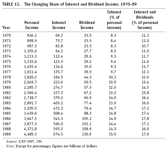
Lindsey’s discussion agrees that if the changes in the economy actually slanted income toward interest, dividends, and capital gains instead of wages and salaries, that would constitute a shift toward the rich (and very rich), as Krugman has calculated. Lindsey’s response is to argue that most of the increase in interest income had occurred between 1977 and 1981.
The interest share of personal income peaked in 1985 at 14.4 percent of income. Thus three-quarters of this windfall to the rich occurred before Reagan took office. Like the poverty rate, interest income as a share of personal income fell in the latter half of the Reagan presidency.70
Table 13 tracks personal income, personal interest income, and personal dividend income between 1970 and 1989. According to this information, interest and dividend income as a percentage of personal income declined by less than 1 percent between 1986 and 1988 and then jumped to a level above 1986 in 1989. It is important to note that the decline between 1986 and 1988 left that percentage much higher than it was when Ronald Reagan took office.71 Thus, in contrast to the impression created by Lindsey’s statement, the increase in interest income as a percentage of personal income stayed at historically high levels throughout the Reagan recovery, rising to its highest percentage in the last year of that recovery. This is not surprising because the key macroeconomic policy constant for the entire period from 1979 to 1990 was tight money imposed by the Federal Reserve. As shown back in chapter 8, the real interest rate rose in 1988 and 1989 as the Fed suggested that pursuit of a zero rate of inflation was not an unreasonable goal.
Robert Bartley introduced two major ways of challenging the general picture of increased inequality. First of all, he argued that even though income distribution might look very unequal, consumption expenditures by different groups within the income distribution were much more nearly equal than incomes. For example, in 1989, the lowest 20 percent received on average $5,720 in pretax income but on average spent $12,119. Bartley suggests that if we are concerned about the well-being of people, the amounts spent on consumption by each group in the income distribution would be a much better measure than the income figures.72 He then attacks the trends in income distribution in the following way:
Between 1983 and 1989, the real income of the bottom quintile rose 11.8 percent, while the real income of the top quintile rose by 12.2 percent. By contrast, between 1979 and 1983, the real income of the bottom quintile fell 17.4 percent, while the real income of the top quintile rose 4.8 percent. Once the tide actually started to rise, in other words, it did lift all boats.73
In other words, he is arguing that the divergence of the income distribution is not the result of the Reagan administration policies but of the period between 1979 and 1983 when the anti-inflation policy of the Federal Reserve coupled with the 1981–83 recession caused all of the problems experienced by low-income people. The problem with this argument is that the criticism leveled by Krugman and others is of the long-term trends, which, as we have argued in chapter 8 must be measured from peak to peak of the business cycle. Even using Bartley’s numbers one can note that despite the “seven fat years” of 1983 to 1989, the real income of people in the bottom 20 percent of the population had not risen enough to make up for the loss between 1979 and 1983. Meanwhile, those in the top 20 percent experienced increases in real income over the entire period, including the recession years.
One counterargument emphasized by Alan Reynolds of the National Review is that the evidence about the divergence between income groups is irrelevant because there is a great deal of social mobility between these groups. In other words, it doesn’t matter if over a decade the ratio between the average income in the top group and the average income in the bottom group increases, if over the same period, a large number of individuals in the bottom group will have moved up to a higher group. Reynolds argued that based on a study by the Department of Treasury,
86 per cent of those in the lowest fifth in 1979, and 60 per cent in the second fifth, had moved up into a higher income category by 1988.. . . Similar research by Isabel Sawhill and Mark Condon of the Urban Institute found that real incomes of those who started out in the bottom fifth in 1977 had risen 77 per cent by 1986.74
The problem with the Treasury study is that it was restricted to people who paid taxes in all ten years. This clearly biases the sample toward those who are economically successful. The reference to Sawhill and Condon is only a partial report on what these Urban Institute scholars wrote in June 1992. It is true that the real income of the total sample of individuals in the bottom 20 percent in 1977 rose 77 percent by 1986. However, only half of the sample had actually raised their incomes enough to get out of the bottom 20 percent. The fact of social mobility does not contradict the trend toward increased inequality. The only way that would be possible would be if the amount of social mobility were to increase along with the inequality. Sawhill and Condon argued that there is no evidence of increased social mobility and hypothesized, therefore, that with inequality increasing and social mobility not increasing, lifetime incomes would become more unequal.
To partially test this hypothesis, we averaged the total income of each individual in our sample over two ten-year periods, 1967–76 and 1977–86, and then ranked all individuals into five quintiles in both periods. . . . By averaging income over a ten-year period, we take account of each person’s mobility over that period and get a more permanent measure of income. . . . In the second period . . . there was greater inequality. This finding suggests that lifetime incomes are becoming more unequal.75
They conclude,
Although the poor can “make it” in America and the wealthy can plummet from their perches, these events are neither very common nor more likely to occur today than in the 1970s.76
This conclusion is in direct contradiction to the implications Reynolds attempted to draw from their data.77
For a final piece of evidence, it is useful to turn to the work of Timothy Smeeding, Greg Duncan, and Willard Rodgers. In order to determine whether the apparent polarization of the income distribution is, in fact, shrinking the middle class, the kind of data reported regularly by the census is insufficient because it does not capture what happens to the same people over time. The Sawhill-Condon analysis does attempt to do this, and their results are suggestive. However, the Smeeding-Duncan-Rodgers study, cleverly entitled “W(h)ither the Middle Class?” makes a major contribution to our understanding because it tracked adults between twenty-five and fifty-four years of age over a period of twenty-two years. The sample was the Panel Study of Income Dynamics, a yearly survey of a large number of adults from 1968 to the present. Smeeding Duncan and Rodgers surveyed the income changes experienced by individuals who remained within that age group between 1967 and 1988 (the income years reported by the 1968 and 1989 interviews).
They began by defining as middle class anyone whose income in a given year was above that received by the bottom 20 percent in 1978 and below that received by the top 10 percent in 1978 (the middle of the period). Thus, the middle class was defined by an absolute measure of income.78 Smeeding, Duncan, and Rodgers then tracked their sample between 1967 and 1986. Between 1970 and 1977, the middle class was between 71 and 75 percent of the total sample. Beginning in 1977 and continuing through the rest of their survey years, the middle class does shrink. Between 1977 and 1981, this is largely due to the big increase in the percentage of the sample who are poor. After 1981, the reduction in the percentage that are poor does not counteract the increase in the percentage that are in the highest income group. On balance, before 1980 the poor had more chances of climbing into the middle class, while the middle class was less likely to fall into the lower income group than after 1980. People leaving the middle class before 1980 were just as likely to rise into the top income group as to fall into the bottom group, whereas after 1980 they were more likely to fall than to rise.79
In analyzing the most significant causes of the changing patterns after 1980, the authors identify the earnings of men as crucial.
[T]he favorable transitions involving men’s earnings . . . showed that they were . . . associated with higher rates of pay. . . . Downward transitions for men were more likely to result from changes in hours—job loss and unemployment—than declining rates of pay.
The widening of the income distribution and the withering of the middle class are mainly associated with growing inequality in men’s earnings—in particular wage changes.80
This supports the analysis presented in the reports of the Economic Policy Institute, The State of Working America, which were referred to above. Just as Paul Krugman and Kevin Phillips argued, the rising tide of the 1980s did not lift all boats.
One group of boats that had less chance of being lifted were those filled with African Americans. Between 1979 and 1989, the ratio of real median income of black men fifteen years or older to white men of the same age went from 61.9 percent to 60.4 percent. In absolute terms, black men earned less in 1989 than in 1979. For black women fifteen and older, the ratio to white women’s income went from 91.1 percent to 80.3 percent, though both black and white women experienced absolute increases in median real income.81
When we focus on wage differentials, we see that the black-white earnings gap increased from 10.9 percent in 1979 to 16.4 percent in 1989, for an annual increase of 0.6 percent. Interestingly, even ominously, the most significant increase in the earnings gap occurred among college graduates. For this group, the earnings gap had declined between 1973 and 1979, only to rise at an annual rate of 1.6 percent for the next decade, from 2.5 percent to 15.5 percent.82 In a study by John Bound and Richard Freeman, the rise in the earnings gap is decomposed into various causal factors.
Among the workforce as a whole, the increase in blacks’ wage disadvantage arises from the fact that the occupations and cities in which blacks are concentrated had lower wage growth, that blacks became relatively more concentrated in low-wage industries and nonunion settings, and that blacks were particularly disadvantaged by the failure of the minimum-wage threshold to keep up with inflation.83
Among the college graduates, 19 percent of the increased earnings gap can be attributed to the concentration of black college graduates in occupations experiencing lower than average wage growth. All other elements contribute 7 percent or less, leaving fully 59 percent of the earnings gap unexplained. The authors of the State of Working America suggest that “greater, or more potent, discrimination as well as weaker government enforcement of anti-discrimination laws may have played an important role.”84 They note that this rise in the racial wage gap occurred at the same time that the gap in test scores has been narrowing.85
This rise in black-white inequality is somewhat paralleled by the trend in black-white unemployment rates. The ratio of black to white unemployment in 1979 was 2.41, and in 1989 it had risen to 2.53. However, among men twenty years and older the ratio was unchanged.86 Thus it appears clear that increased inequality between blacks and white is not caused by increased black unemployment but by an increase in the differences of earnings. As interest, dividends, and capital gains helped increase the inequality of income among the population as a whole, we should assume that the fact that the black population on average derives much less of its income from interest, dividends, and capital gains than the rest of the population played some role in the black-white income gap as well.
The increase in inequality between blacks and whites, especially among college graduates, suggests that one of the major complaints about the 1980s, namely that affirmative action programs had promoted blacks at the expense of whites, particularly in the professions, has no basis in reality. As a higher percentage of blacks with higher (test score) qualifications graduated from high school and college, they experienced a decline in earnings relative to their white counterparts, over half of which was unexplained by causes other than discriminatory behavior. We might also remind the reader that the decade of the 1980s saw declining enforcement of affirmative action and other antidiscrimination programs.
The Decline in Leisure
But how is it possible that declining hourly wages and increased inequality can be consistent with rising median incomes? Except for the bottom 20 percent, all families realized some increase in real income over the decade 1979–89 (though the second 20 percent experienced an increase of less than 1 percent over the entire decade!).87 They experienced increases in real incomes because on average people worked more hours in 1989 than they did in 1979, and the participation of married women in the labor force continued to increase.88 This actually marked the continuation of a much longer trend noted by the 1991 best-seller The Overworked American by Juliet Schor. Schor and her colleague Laura Leete-Guy discovered that after declining for almost one hundred years, the average work week began to rise in the 1940s and continued rising right up through the 1980s.89 This trend led to such a decline in leisure hours for average working families that for the first time public opinion surveys showed that large percentages of the population would willingly give up part of their paychecks for more leisure time.90
The rise in the number of hours of work supplied by individuals to the marketplace in the face of declining hourly wages calls into question a fundamental premise of traditional economic analysis. The supply of any item, toothbrushes, cars, and the factor of production labor, is supposed to fall if the price paid for it (in the case of labor, that would be the wage) falls. Yet in the 1979–89 period we seem to have a perverse situation where declining wages are associated with rising numbers of hours supplied. The explanation is that the labor market is fundamentally different from other markets. In the case of most products, rising prices can attract new producers into the market, and falling prices can send producers leaving the market to produce and sell other things. In the case of the factor of production labor, most individuals have no alternative factors of production to sell if they cannot get enough for their labor. For most people, it is not possible to respond to declining wages by quitting and making a living selling something else. Some people with large amounts of assets that can be sold or invested do have the opportunity of “substituting” the supply of some other factor of production for their labor in the marketplace. These are a small minority of the population. Most people rely solely on their ability to work. If the wage they receive shrinks over time, many will respond by attempting to preserve their standard of living by working longer hours if they cannot switch to a higher-paying job.
This fact about the labor market explains why the big increase in the supply of labor from women (the labor force participation rate) occurred during the 1970s, years when the high marginal tax rates were supposedly discouraging women from entering the labor force. Though the participation of women in the labor force continued to expand during the 1980s, the rate of increase was much slower, despite the introduction of the supply-side incentives in ERTA in 1981.
There is another important fact about the labor market that the recent experience of the unwilling surrender of leisure highlights. People do not enter the labor market with the full freedom of other sellers. If I am a farmer, I have the right to determine how much of a crop I will grow and how much of my crop to offer for sale. The same is true if I am a retailer or a manufacturer. I determine how much inventory to stock and how much of a given product to produce and I determine when and in what quantities I bring them to market.
A worker offering to sell one’s labor usually is faced with three choices: work full time, part time, or not at all. In addition, what constitutes full or part time will be decided by the employer (and a union in rare cases). The reduction in the average work week that occurred over the one-hundred-year period from the early nineteenth century through the 1930s occurred as a result of long, difficult, and concerted efforts by labor unions, sometimes aided by government policy, to force business as a whole to change what constituted full-time work. Beginning with the 1940s, the labor movement abandoned efforts to shorten the work week further, and by the end of the 1970s unions had become quite weak in setting national wage and hours policy.91
Meanwhile, American business appears to have decided that for a variety of reasons, it would be more profitable to hire three people to work eight hours than to hire four people to work six hours. One might wonder what the difference would be if the hourly wage were the same, but Schor makes some very telling points about the rationale of business. First, she suggests that mechanization and the need to train labor help explain the bias from business in favor of longer hours.
Employers typically prefer to hire fewer workers and keep them on long schedules because they cannot count on finding additional workers of comparable quality and experience.92
The more complicated the machines, the higher the fixed costs involved in hiring and training and the more incentive there is to spread those fixed costs over more hours of work per worker.
Then there is the need to discipline labor that arises from the need to get workers to cooperate, as we have mentioned a number of times. One technique, which Schor traces to Henry Ford’s famous five-dollars-a-day wage, is something traditional economics would find irrational, the creation of employment rent—in lay terminology, “overpaying” workers substantially. Technically, any payment over and above the wage necessary to get workers to join your company constitutes rent. Going back to David Ricardo, rent is a pure return to scarcity rather than an actual payment for a service. So what was so scarce about a semiskilled factory worker on Henry Ford’s assembly line? Their willingness to stay on the job and work on an assembly line at its pace. The scarce item that earned the rent was docility. Once disciplined by overpayment (five dollars a day more than doubled the going wage rates in auto plants), workers could be subjected to speedups and other methods of boosting production. Schor concludes that “the development of employment rents played a major role in stabilizing and containing problems of labor discipline in twentieth century America.”93 Longer hours, with time and a half for overtime, raises the employment rent and ties workers even more completely to their jobs. In the post–World War II period, the rise of fringe benefits as a percentage of the cost of employee compensation introduces an even larger fixed cost of employing a worker beyond the training costs associated with mechanization. Three workers working eight-hour days is now much less expensive than four workers working six-hour days because that’s one less package of fringe benefits.
Paradoxically, Schor notes that the decline in leisure has occurred as the inability of the economy to provide full-time employment for those who wanted work became more apparent. Since 1969, measured unemployment, discouraged employment, and involuntary part-time work has increased on average over each full business cycle. Schor argues that this has created another bias in the economy in favor of long hours for fewer workers. If workers reduced their hours on average, more jobs would be available. If this happened for the economy as a whole, the rate of unemployment would decline precipitously. From a supply-and-demand analysis, again, one might wonder why business would care (ignoring for a moment fixed costs like fringes). The answer, of course, is that very low unemployment rates lower the employment rent associated with any one particular job. This reduces the “club” that business can wield in the conflict-driven labor market. Schor notes that when American labor proposed a thirty-hour week during the depression, the business community mobilized all its political muscle to induce President Roosevelt to oppose the law that had already passed the Senate. The behavior of the business community and their supporters in the economics profession suggests that full employment is incompatible with American-style capitalism, and the push to extend the hours of those working that helps make some significant percentage of the workforce superfluous fits into that pattern.
Conclusion: What Were the Real Failures?
Of the major criticisms made of the Reagan-Volcker program, the most well known, the high deficit and debt, appear to have done no damage to the economy. However, government purchases in the defense area to the neglect of infrastructure and education do appear to have had a negative impact on productivity and income growth. The combination of deregulation and lax enforcement led to the disastrous savings and loan collapse, an example of how commitment to a principle (in this case the superiority of unconstrained markets over regulated ones) without considering the special nature of a particular market can create a serious failure of policy.
Inequality of income presents an interesting problem because there was some dispute as to whether inequality had increased. We believe the evidence establishes a significant increase in inequality and no parallel increase in social mobility. In fact, it appears that over the 1980s it became more likely that people in the middle of the income distribution would fall out into the poverty group rather than rise into the upper income levels. The second problem presented is whether in fact inequality mattered for any reasons other than political reasons. We believe the combination of increased income inequality, slow growth in median income, and decline in leisure led to an absolute stagnation in the incomes and well-being of a significant proportion of the population. The discontent of this group would be a significant element in the politics of the 1990s.