Notes
Chapter 1
1. The first shutdown lasted from November 14 to November 19, 1995 (New York Times, November 20, 1995, 1). The second began on December 16 (New York Times, December 17, 1995, 1; for details on what was shut and what wasn’t, see p. 40). See also Congressional Budget Office, The Economic and Budget Outlook: Fiscal Years 1997–2006 (Washington, DC: Government Printing Office, 1996), 9.
2. An article in the Wall Street Journal pointed out how much President Clinton had moved since the previous year. Whereas the previous year’s (February 1995) budget proposal had projected deficits of $200 billion per year for the foreseeable future and contained five years of spending cuts totally $81 billion, the 1996 proposal had increased the projected cuts to $234 billion, permitting a deficit of zero by 2002 providing the economy remained at a steady rate of growth. With this reversal, President Clinton had surrendered to the Republicans. See Jackie Calmes, “Clinton’s Fiscal ’97 Budget Reflects Major Shift toward Ending Deficits and ‘Big Government,’” Wall Street Journal, February 6, 1996, A16.
3. For details of that bill, see U.S. House of Representatives, Committee on Ways and Means, 1996 Green Book: Background Material and Data on Programs within the Jurisdiction of the Committee on Ways and Means (Washington, DC: Government Printing Office, 1996), 1325–1418.
4. The most significant cuts in the 1995 budget that Congress had passed and that the president had vetoed were in the Medicare and Medicaid programs. To measure such cuts, the Congressional Budget Office (CBO) starts with a “baseline budget.” This budget indicates how much it would cost to maintain current services over the period of time being considered, based on the CBO’s estimates of costs and revenues, if no changes were enacted. Then the changes passed by Congress are measured against this baseline. This procedure is the source of the argument as to whether these are cuts or merely slowing the growth of spending. In fact, slowing the growth of spending makes it impossible to provide services at the current level to the growing population eligible for those services (the retired, the poor, the disabled in the case of Medicare and Medicaid) with the increased cost of providing those services over time. In December 1995, compared to the CBO baseline, recalculated according to the most recent predictions about the economy’s next six years, the budget passed by Congress would have reduced federal spending by approximately $401 billion, of which approximately $359 billion would have been in Medicare and Medicaid. It also would have cut taxes approximately $229 billion (Jim Horney, “Memorandum: Updated Estimates of the Balanced Budget Act of 1995,” Congressional Budget Office, December 13, 1995). The 1997 law, by contrast, cut approximately $127 billion in toto while providing a modest $90 billion in tax reductions (and an additional $11 billion in refundable tax credits) through 2002 (see “Budgetary Implications of the Taxpayer Relief Act of 1997” and “Budgetary Implications of the Balanced Budget Act of 1997” in letter, June E. O’Neill, director, Congressional Budget Office, to Franklin D. Raines, director, Office of Management and Budget, August 12, 1997.)
5. For an analysis of Clinton’s goals and methods on the road to this compromise see Martin Walker, “He Stoops to Conquer: Clinton’s Budget Pact Shows His Messy Means to a Grand End,” Washington Post, May 11, 1997, C1, C5. For initial coverage of the agreement, see the New York Times, July 30, 1997, A16, A17.
6. The Employment Act of 1946 states that
it is the continuing policy and responsibility of the Federal Government to use all practicable means, consistent with its needs and obligations and other essential considerations of national policy with the assistance and cooperation of industry, agriculture, labor, and State and local government, to coordinate and utilize all its plans, functions, and resources for the purpose of creating and maintaining, in a manner calculated to foster and promote free competitive enterprise and the general welfare, conditions under which there will be afforded useful employment, for those able, willing, and seeking to work, and to promote maximum employment, production, and purchasing power. (Quoted in Stephen Kemp Bailey, Congress Makes a Law [New York: Columbia University Press, 1950], 228.)
The responsibility to “promote maximum employment” has been interpreted as requiring efforts to respond to the increase in unemployment that accompanies recessions. In 1978, this law was amended by the Full Employment and Balanced Growth Act to include a specific target of 4 percent unemployment.
7. There is a significant strand in economic analysis that suggests that paying the unemployed compensation may actually delay workers’ finding new jobs because the benefit subsidizes the time without a job and reduces the urgency with which they look. See Martin Feldstein, “The Economics of the New Unemployment,” Public Interest 33 (1973): 3–42. Similarly, there is a strongly held view, exemplified by the work of Charles Murray in Losing Ground: American Social Policy, 1950–1980 (New York: Basic Books, 1984), that providing cash assistance to the poor as welfare actually causes poverty rather than reducing it. This point of view became the intellectual justification for the Republican proposals that led ultimately to the abolition of Aid to Families with Dependent Children, the program that provided a federally guaranteed cash grant to children in poor, single-parent families.
8. To give one example, total federal spending as a percentage of total economic activity (gross domestic product) stayed around 10 percent for the entire decade of the 1930s, rose to around 15 percent after World War II, hovered around 19 percent from the end of the Korean War till the late 1960s, and climbed to near 21 percent by 1979 (Economic Report of the President 1996 [Washington, DC: Government Printing Office, 1996], 368; henceforth these annual reports are abbreviated ERP, with the year indicated). Considering total government expenditures (including state and local outlays for things like police, fire, education, and public assistance), we see an upward trend from 25 percent of total activity to 30 percent between 1960 and 1979.
9. The United States Central Bank consists of a system of twelve regional federal reserve banks whose actions are controlled by a seven-member Board of Governors in Washington appointed by the president (and subject to confirmation by the Senate) for fourteen-year terms. However, for the most important policy decisions, the controlling unit is the larger Federal Open Market Committee, which consists of the seven governors and the presidents of five of the regional banks (with the president of the New York Federal Reserve Bank always among the five). The actions of the Federal Reserve System are completely independent of the three branches of government, except that Congress may change the rules by legislation at any time. The president and secretary of the Treasury have no direct influence on Federal Reserve policy. All they can do is make speeches and attempt persuasion. A president wanting to force a change in policy would have to propose legislation to Congress. For a massive study of both the history and recent experience of the Federal Reserve System, see William Greider, The Secrets of the Temple: How the Federal Reserve Runs the Country (New York: Simon and Schuster, 1987).
10. A more detailed table, which goes back only to 1968, is provided in the 1996 Green Book, 1321. Programs redistributing income on the basis of need for medical, food, and cash assistance went from 4.9 percent of the federal budget (in 1968) to 8.5 percent of the budget in 1978. Note that these are fiscal years, not calendar years. The fiscal year went from June of the previous year to the end of May of the numbered year until 1976; and from 1977 on, from October 1 of the previous year to the end of September of the numbered year. Thus, “fiscal 1968” was from June 1, 1967 to May 31, 1968. “Fiscal 1978” was from October 1, 1977 to September 30, 1978.
11. ERP 1997, 391.
12. The Congressional Budget Office analysis of the 1997 law shows a cut in Medicare spending of $115 billion in the years 1998 to 2002 over the predicted path of spending if no changes were to occur. See letter, June E. O’Neill, director, Congressional Budget Office, to Senator Pete V. Domenici, chairman, Committee of the Budget, United States Senate, July 30, 1997, table 4.
13. Daniel P. McMurrer and Isabel V. Sawhill, “Economic Mobility in the United States,” Urban Institute no. 6722 (1996).
14. After the Republican success in the 1994 congressional elections, the Contract with America was published in book form, edited by Ed Gillespie and Bob Schellhas (New York: Times Books, 1994).
15. Representative Meek had asserted that
in 1980 a group of Republican candidates came to the Capitol steps and pledged that, if elected they would enact a supply-side miracle that would raise defense spending, cut taxes across the board, and still eliminate the deficit in 4 years. . . . They rammed their supply-side quick-fix through the Congress, and claimed it would solve all of our problems. . . . Their latest contract calls for: Another round of defense spending increases and a longer list of pie in the sky tax cuts.
What they do not tell us is that their contract will do two other things: First blow a $1 trillion hole into their balanced budget promise; and second, produce another tax windfall for the wealthy while leaving the middle class and the poor behind. (Congressional Record [September 29, 1994], 10254)
16. For example, see the following remarks by Speaker-designate Newt Gingrich on November 11, 1994: “It is impossible to take the Great Society structure of bureaucracy, the redistributionist model of how wealth is acquired, . . . and have any hope of fixing them. They are a disaster. They . . . have to be replaced thoroughly from the ground up” (Contract with America, 189).
17. It should be noted that some scholars and not a few citizens believe that this theoretical analysis is just a veneer behind which the true purpose of economic policy is to redistribute income and opportunity to those already in power, who have always been able to manipulate the political system to their ends. Thus, the role of government has always been rather extensive, and the cry for less government involvement always ignores the things government does to subsidize investments and profits of already large and successful enterprises. (On this point, note the increase in government activity and spending related to law enforcement, the punishment of criminals, and the defense establishment promised by the Republicans in the Contract with America, 37–64, 91–113.) This book will allude to this alternative point of view at times, but for the most part, we will conduct our discussion based on the mainstream analysis. The reason is that even if this alternative explanation of economic policymaking were true (and there is plenty in the historical record consistent with it), the changes in policy during the 1980–97 period are significant and worth exploring on their own terms. Second, the debates in the mainstream do not credit this alternative approach, and in the interest of dialogue with that mainstream, it is essential to accept some of the most basic premises, at least for the sake of the current discussion.
18. The federal budget deficit fell from $255 billion in fiscal 1993 to $22 billion in fiscal 1997. See Robert Pear, “Budget Heroes Include Bush and Gorbachev,” New York Times, January 19, 1998, A12. See also ERP 1998, 372. Federal spending fell from 21.7 percent of total income to 21.1 percent between fiscal 1992 and 1996 (ERP 1997, 300, 391).
19. The economic proposals are contained in the following promised laws: “The Fiscal Responsibility Act . . . The Personal Responsibility Act . . . The American Dream Restoration Act . . . The Senor Citizens Fairness Act . . . The Job Creation and Wage Enhancement Act” (Contract with America, 9–10; see also 17–18). The specific proposals in these laws were a balanced-budget amendment to the Constitution, a denial of welfare to minor mothers, a rigid two-years-and-out limit on welfare eligibility and a cut in the dollars available for welfare, a five-hundred-dollar-per-child tax credit for all taxpayers making up to two hundred thousand dollars a year, an increase in the amount of money Social Security recipients can earn while collecting their pensions, a repeal in the 1993 tax increases on some Social Security income, a cut in taxes on business income including capital gains, and a reduction in government regulation of business and federal regulation of the states.
20. For the agreement, see Jerry Gray, “Congress and White House Finally Agree on Budget 7 Months into Fiscal Year,” New York Times, April 25, 1996, A1, B13.
21. The marginal tax rate is the percentage of the next dollar you stand to earn by, say, accepting a higher-paying job that you would have to pay in taxes. With a tax system that starts with some income free of taxation and then has a series of rising rates (such as our federal income tax system), the average tax rate is just the total level of taxes divided by total income. The marginal rate will always be higher than the average rate so long as some income is tax free (and therefore subject to a zero rate). It is the contention of some economists, including Lindsey, that high marginal tax rates discourage productive economic activity. See Lawrence B. Lindsey, “Simulating the Response of Taxpayers to Changes in Tax Rates,” Ph.D. diss., Harvard University, 1985. For a concise, less technical discussion, see Lawrence B. Lindsey, The Growth Experiment: How the New Tax Policy Is Transforming the U.S. Economy (New York: Basic Books, 1990), 53–80.
22. This is the conclusion ultimately reached by Samuel Bowles, David M. Gordon, and Thomas Weisskopf in After the Wasteland: A Democratic Economics for the Year 2000 (Armonk, NY: M. E. Sharpe, 1990). See especially pp. 121–69. For a short summary of the regressive tax changes, see Lawrence Mishel and Jared Bernstein, The State of Working America, 1994–1995 (Armonk, NY: M. E. Sharpe, 1994), 93–108.
23. A supporter of Reagan-style tax cuts even before Reagan was elected president, Jude Wanniski wrote a book (How the World Works [New York: Touchstone/Simon and Schuster, 1978]) arguing that the ups and downs in all of world history can be traced to regimes of low versus high taxation.
24. See for example, Spencer Abraham, “The Real 1980s,” The World and I, April 1996, 94–100. For counterarguments see Gary Burtless, “Tax-Cut Potions and Voodoo Fantasies,” The World and I, April 1996, 100–102; and Michael Meeropol, “A Smoke Screen for Brutal Interest Rates,” The World and I, April 1996, 102–3. See also Alan Reynolds, “Clintonomics Doesn’t Measure Up,” Wall Street Journal, June 12, 1996, A16.
25. Still others deny that the distribution of income has become more unequal.
Chapter 2
1. “Oeconomicus,” Xenophon in Seven Volumes, trans. E. C. Marchant (Cambridge: Harvard University Press, 1968), vol. 4. The original conception of the ancient Greeks and Romans was very practically related to personal management of one’s property (vii).
2. However, as noted in the previous chapter, income distribution is very important as a political issue. There is also an argument from the radical tradition in economics that the distribution of income and wealth has an important impact on economic growth. See pp. 59–63.
3. Of course this is in societies like the United States. In most traditional societies (and human beings lived in such traditional societies for hundreds of thousands of years before settled agriculture and civilization developed more complex organizations for producing food, clothing and shelter) cooperation occurs without modern-style leadership. True, there was a designated leader, but tasks were carried out based on tradition, not direct orders. Even in the United States and other modern economies, the leadership of certain organizations, such as cooperatives and partnerships, is not so hierarchical. Here voluntary cooperation is much more explicit, and, in fact, in many cooperatives extensive rules govern that cooperation.
4. Harry Braverman, Labor and Monopoly Capital (New York: Monthly Review Press, 1974), 54–69 and 85–151.
5. In fact, even in the classic management literature, both the necessity of imposing order and maintaining control (the Marxist emphasis) and the fostering of a cooperative spirit coexist. For example, Henri Fayol, who published Administration industrielle et generale in 1916 (General and Industrial Management, trans. Constance Storrs [London: Isaac Pitman and Sons, 1949]), listed fourteen universal principles of management. Though most of the principles emphasize centralizing control over the work process (and therefore over the workers) in the hands of management (19–40), there is an intriguing fourteenth point, “Esprit de corps . . . Harmony, union among the personnel of a concern, is great strength in that concern” (40). In the late 1920s, the famous Hawthorne studies discovered (quite inadvertently) that varying physical surroundings of workers had much less important an effect on how well and hard they worked than did the attitudes of the workers themselves. Elton Mayo quoted from a private internal report on these studies as follows,
The changed working conditions have resulted in creating an eagerness on the part of operators to come to work in the morning . . .
The operators have no clear idea as to why they are able to produce more in the test room; but . . . there is the feeling that better output is in some way related to the distinctly pleasanter, freer, and happier working conditions . . .
. . . much can be gained industrially by carrying greater personal consideration to the lowest levels of employment. (The Human Problems of an Industrial Civilization [New York: Viking, 1960], 65–67)
The inescapable conclusion of the Hawthorne Studies was that emotional factors related to morale were more important in determining the productivity of workers than physical factors.
Mary Parker Follet, lecturing in 1933, felt that she had discerned among the most forward-looking businesses the practice of developing collective responsibility, not only between different branches of the administration of a business, but down to the workers on the shop floor,
wherever men or groups think of themselves not only as responsible for their own work, but as sharing in a responsibility for the whole enterprise, there is much greater chance of success for that enterprise . . . when you can develop a sense of collective responsibility then you find that the workman is more careful of material, that he saves time in lost motions, in talking over his grievances, that he helps the new hand by explaining things to him and so on. (Freedom and Co-Ordination, Lectures in Business Organization [New York: Garland, 1987], 73)
I am indebted to my colleagues Julie Siciliano and Peter Hess of the Department of Management at Western New England College for calling my attention to these sources.
6. In the context of environmental degradation and fears of world overpopulation, to state that growth appears to be have become permanent since the Industrial Revolution might be considered the height of hubris. I do not want to underestimate the dangers posed by environmental deterioration. However, it is a fact that the increased knowledge that has created the technology that is endangering our planet has also given us the potential information necessary to harness the technology and, in the words of the ecologist Barry Commoner “make our peace” with the planet (Making Peace with the Planet [New York: Pantheon, 1990]).
7. The importance of government in stimulating private investment with subsidies and other incentives should not be underestimated. For example, at the height of the laissez-faire approach to free enterprise during the nineteenth century, the U.S. government provided a tremendous subsidy to the railroads. First the government used the armed forces to defeat the Plains Indians and remove them from their land. Second, the government granted thousands of acres of land to the railroads along their right of way, land that the railroads were able to sell quite profitably. Virtually every major surge in investment in the United States can be traced to indirect or direct subsidies as a result of government activity, whether making war, building roads, or the like. Nevertheless, it is true that the actual spending of the investment funds is done by a private entity.
8. Contract with America, 23.
9. H. Ross Perot in United We Stand emphasized the interest burden on the federal taxpayer of the four-trillion-dollar national debt. He asserted,
By 2000 we could well have an $8-trillion debt. Today all the income taxes collected from the states west of the Mississippi go to pay the interest on that debt. By 2000 we will have to add to that all the income tax revenues from Ohio, Pennsylvania, Virginia, North Carolina, New York and six other states just to pay the interest on that $8 trillion.
Central to the criticism leveled by Perot at the political leaders is a linkage between the unacceptable behavior of the economy in the 1990s and the ballooning national debt. In his very first chapter, he begins by mentioning some large layoffs. He then mentions the national debt and its growth every day as a result of the government deficit and concludes, “Does anyone think the present recession just fell out of the sky?” (United We Stand: How We Can Take Back Our Country [New York: Hyperion, 1992], 5)]. The reader is left with the inescapable conclusion that Perot wants us to believe the large debt caused the recession. We will explore these and other arguments about the alleged burdens of deficits and debt below. See pp. 43–44, 162–63, 170–74.
10. In Restoring the Dream, ed. Stephen Moore (New York: Times Books, 1995), 65–81, the House Republicans continue their arguments and promises made in the Contract with America. Their laments about the damage being done by budget deficits adds virtually nothing to what was said in the first volume. There is a reference to the absorption of national savings, the problem just referred to of “crowding out” private investment. The only other specific problems involve the increased percentage of federal spending devoted to interest payments on the debt and a reference to the fact that a rising percentage of the debt is held by foreigners. Both of these “problems” are not as serious as they make them out to be and are discussed on p. 170 and tables N-13 and N-14. Everything else in these pages is just rhetoric. Readers skeptical of the assertions made here may want to consult any textbook on the principles of economics. There is usually a chapter on deficits and government debt. A more sophisticated but highly accessible analysis can be found in Robert Eisner’s The Misunderstood Economy: What Counts and How to Count It (Boston: Harvard Business School Press, 1994), 89–119. See also James K. Galbraith and William Darity Jr., “A Guide to the Deficit,” Challenge, July–August 1995, 5–12. For a recently published work that examines the intellectual history of American concern with budget deficits in great detail and argues for other damage that could potentially be done by some forms of deficit spending, see Daniel Shaviro, Do Deficits Matter? (Chicago: University of Chicago Press, 1997), esp. 28–150.
11. There is a school of economics known as the “public choice” school whose most prominent member, James Buchanan, received the Nobel Prize in economics in 1989. This school contends that there is an inexorable political pressure for government to expand its involvement in the economy based on the self-interest of government officials, elected and appointed, as well as the intensity of desire on the part of beneficiaries of government largesse. According to Buchanan, the future generations who must pay interest on the debt contracted before they were born have no political say in the decisions made by their grandparents, and thus the deck is politically stacked against them. In Democracy in Deficit: The Political Legacy of Lord Keynes (New York: Academic Press, 1977), Buchanan together with Richard Wagner blamed deficit spending for the ability of government to increase its spending in the economy. “Elected politicians enjoy spending public monies on projects that yield some demonstrable benefits to their constituents. They do not enjoy imposing taxes on these same constituents. The pre-Keynesian norm of budget balance served to constrain spending proclivities. . . . The Keynesian destruction of this norm . . . effectively removed the constraint” (93–94). Later on, they assert that the “bias toward deficits produces . . . a bias toward growth in the provision of services and transfers through government” (103). For a detailed examination of the “public choice” school, see Shaviro, Do Deficits Matter? 87–103.
12. This was baldly admitted by Murray Weidenbaum, the first chairman of the Council of Economic Advisers under President Reagan. At a discussion at the American Enterprise Institute, he candidly explained that concern over the deficit was necessary to counter pressure for increased government spending.
- dr. weidenbaum: I’d like to offer, hopefully, some insight into the continuing concern . . . about deficits. I think the underlying concern is . . . to control the growth of government.
- And we measure that most conveniently by outlays. Surely the pressure for government spending growth is omnipresent. What is the counter pressure? In the legislative process . . . we’re led back to the concern over deficits. . . .
- Dr. Stein [Herbert Stein, former chairman of the Council of Economic Advisers, then resident scholar at the AEI]: But aren’t you worried that the whole trend of this discussion is reducing the inhibitions about running deficits, and therefore, weakening this restraining force against government spending.
- Dr. Weidenbaum: Maybe that’s why I made my comment.
- Dr. Stein: Well, that’s a good reason to make the comment but something more needs to be said then. That is, you need to reestablish some defensible reason for not having deficits. If you’ve now told us that they don’t cause inflation, they don’t crowd out. You see, it is not sufficient, as we know, for a group of economists to sit around and say, “Well, a deficit of a hundred billion dollars doesn’t have these adverse effects,” because you’re dealing with a bunch of Congressmen out there, and if we say 100 billion is OK, they will ask why not 200 or why not 300.
- They have a certain feeling about zero [that is, a balanced budget]. Zero is an intuitively appealing number. But we haven’t found any other intuitively appealing rule, and that’s what we’ve been missing. (American Enterprise Institute, “Public Policy Week,” mimeo transcript, December 8, 1981, qtd. in Robert Bartley, The Seven Fat Years [New York: Free Press, 1992], 191–92)
13. See Milton Friedman, Capitalism and Freedom (Chicago: University of Chicago Press, 1962) and his collaborative work with Rose Friedman, Free to Choose: A Personal Statement (New York: Harcourt Brace Jovanovitch, 1980).
14. Qtd. in Conald Bedwell and Gary Tapp, “Supply-Side Economics Conference in Atlanta,” Economic Review of the Federal Reserve Bank of Atlanta 57 (1982): 26.
15. See the quotations from Buchanan in note 11.
16. In fact there is another way a government can finance deficit spending, called “running the printing presses.” It involves printing money and using it to pay for what the government needs. Such behavior had its origins in the days when governments collected precious metals and turned them into coins at the mint. In order to get more coins out of the precious metal, the mint was ordered to mix in some cheap metal with the gold or silver. This process was known as “debasing the currency,” and the result was that the regime’s coinage came into ill repute and individuals did not want to accept it at face value. Recent history has shown that wholesale resort to printing money to finance government expenditures leads to very rapid inflation—such as in Germany in 1922, when millions of marks were needed for a loaf of bread. This result has led many to argue that it is irresponsible to meet government spending needs by printing money over and above tax revenue. Printing bonds and selling them on the open market is considered more responsible because the rising national debt supposedly acts as a check on too much money creation. However, judicious printing of new money to finance some small percentage of the government budget might very well not lead to hyperinflation. This process, technically known as monetizing the debt, is frowned upon mainly because when the government borrows by issuing bonds, bankers make profits by placing them and investors have a secure place to invest funds. If the government just printed money at a slow enough pace not to accelerate inflation, the bankers would be out their cut.
17. The last time the federal government ran a surplus was in fiscal 1969 (ERP 1994, 359).
18. Contract with America, 23.
19. Eisner, The Misunderstood Economy, 51.
20. This is probably a good place to mention that much of the argument against government spending in general is in reality aimed at government activity that redistributes income. As mentioned in chap. 1, the Contract with America, 91–113, called for increased government spending on national defense. The Republican majority in Congress has since 1994 attempted to reverse the decline in defense spending projected by both the Bush and Clinton administrations, while proposing dramatic cuts in Medicaid, Medicare, and transfer payments to the poor. Even those who rail against spending in general usually treat the defense budget as sacrosanct. Many have argued that this is because the defense budget is an indirect subsidy to large businesses, benefiting the kind of people who make large contributions to members of Congress and whose investment activity is the key to economic prosperity. See chap. 9, n. 18.
21. The National Bureau of Economic Research identifies recessions as periods during which the real GDP (that is, GDP corrected for inflation) falls for two consecutive quarters. Table N-1 combines the NBER’s dating of post–World War II business cycles beginning with the 1948 recession. Each peak marks the end of a period of prosperity and the beginning of a recession. Each trough marks the point where a recession bottoms out and a recovery begins. Table N-1 shows the quarter before and after each peak and trough to give an idea of the way unemployment and capacity utilization rates behave around the peaks and troughs of business cycles. Later we will examine these and many other facts of recent economic history quarter by quarter in the years since 1960.
22. Thus, even though the recovery from the 1990 recession began in the first quarter of 1991, there was not one quarter during the rest of 1991 in which real GDP grew as fast as 2 percent (ERP 1997, 307). Thus, it is not surprising that the unemployment rate actually rose from 6.5 percent in the quarter the recovery began to 7.5 percent in the third quarter of 1992 before it began to decline. Similarly, the capacity utilization rate did not reach 80 percent until the fourth quarter of 1992. This made the 1991 recovery the most sluggish in the postwar period.
23. Note that this is a creation of something physical. Common usage often describes investment as any spending of money to acquire an income-generating asset. By that definition, investment includes buying stocks and bonds as well as physical assets like machines and buildings. For the purposes of describing the impact on aggregate demand, however, we restrict the meaning of investment to physical assets. Purely financial investments actually involve the transfer of ownership rights of already created physical assets and thus are not counted as part of the GDP. This is not to suggest that such financial investments are unimportant; far from it. See pp. 128, 156–57 for some discussion of the impacts of purely financial investments.
24. The public-choice field of economics analyzes that government decision making may not respond to an generalized “public interest” but to the narrow interests of particular constituencies. See James Buchanan, The Demand and Supply of Public Goods (Chicago: Rand McNally, 1968).
25. ERP 1997, 37, 38.
26. ERP 1996, 282.
27. ERP 1997, 389. These are fiscal years.
28. Real investment as a percentage of real GDP fell from 16 percent to 14 percent between 1984 and 1989 (ERP 1996, 282), the federal deficit fell from 5 percent of GDP in fiscal 1983 to 4 percent of GDP in fiscal 1986, and the national debt fell from 57.6 percent of GDP to 39.5 percent of GDP between 1960 and 1969. As a percentage of GDP, this debt is much lower than was the much smaller absolute debt of $271 billion in 1946 (ERP 1997, 389). The ratio of debt to GDP was over 100 percent in 1945 and 1946; that is GDP was actually lower than the national debt in those years.

Chapter 3
1. The rate of growth averaged 4.07 percent between 1960 and 1969 and 2.85 percent between 1970 and 1979.
2. For the periods 1960–69 and 1970–79, productivity growth averaged 2.41 and 1.33 percent, respectively; unemployment averaged 5.58 and 6.21 percent, respectively; and capacity utilization averaged 84.86 and 82.58 percent, respectively.
3. Dean Baker, “Trends in Corporate Profitability: Getting More for Less?” Technical Paper, Economic Policy Institute, February 1996, table 1. A full business cycle begins with a peak and continues through the next trough to the next peak. Alternatively, it can begin with a trough and continue through the next peak to the next trough (see chap. 2, n. 21 and table N-1). The calculation of profit rates is made for the year before each cyclical peak, since the rate of profit usually turns down before the whole economy does. Thus, for example, using the profit rate of 1969 in the 1959–68 business cycle would have actually introduced profit data more appropriate for the next business cycle.
4. I use 1978 as the end point because in 1979 the Census Bureau changed data collections, and a spurt of unanticipated inflation caused median earnings of year-round, full-time workers to fall for that year. I did not want that one year’s experience to skew the data. As it is, the change from the 1960s to the 1970s remains quite striking.
5. A variety of inflation rates are constructed and published by the various branches of the federal government. For the purposes of identifying the misery index, I have chosen the most widely publicized inflation rate, the consumer price index. Not all of the components of the consumer price index apply to all people; for example, a homeowning family with a fixed-rate mortgage is not affected by rising housing costs so long as the family stays put. As many economists will emphasize, however, the knowledge of general inflation has a discomforting impact on people even apart from those higher prices they actually pay.
6. Let’s consider two numerical examples from the period of history covered in this book. Consider a mortgage loan entered into in 1965 with a ten-year maturity. The nominal interest rate in 1965 averaged 5.81 (ERP 1994, 352); the inflation rate (measured by the consumer price index) was 1.6 percent (ERP 1997, 370). If we assume that inflation rate was accurately anticipated by both lenders and borrowers, then the real interest rate these mortgage lenders were expecting was 4.21 percent. Within three years, when the rate of inflation had accelerated to 4.2 percent, the actual real rate of interest received by mortgage lenders was 1.61 percent. In 1969 it was 0.31 percent; in 1970 it was even lower (0.21 percent) because inflation was 5.7 percent. Beginning in 1973 and running through 1975, the rate of inflation was higher than the mortgage rate of interest contracted in 1965. This translated into a negative real interest rate. The borrowers found the reduction in the real burden of their repayment of principal greater than the nominal interest rate they had to pay. The lenders lost real income on those loans.
Now let us consider a mortgage loan contracted in 1981. The nominal rate of interest for a ten-year mortgage averaged 14.7 percent and the rate of inflation in the consumer price index was 10.3 percent. This represented a real interest rate of 4.4 percent, assuming correct anticipation by lenders and borrowers. The rate of inflation deceleration after 1981 was so dramatic that the real burden of the mortgage interest rate rose in 1982 to 8.5 percent and only once fell below 10 percent for the rest of the time till maturity. In other words, borrowers were faced with a real interest burden more than twice as great as they anticipated when they contracted the loan.
7. Some businesses can set their prices and stick to them because they have few competitors, who will most likely match their price rather than provoke a price war. In the most general sense, the distinction needs to be made between businesses that are “price takers” and those that are “price makers.” The earliest empirical work on the significant ability of certain firms to control prices was by Gardner C. Means. He identified industries that responded to the falloff in demand during the Great Depression by keeping prices relatively stable and reducing output. These industries he characterized as those with administered prices (that is, they were price makers) as opposed to those industries (such as agriculture) in which prices fell dramatically but output did not (in other words, price takers) (Industrial Prices and Their Relative Inflexibility, Senate Document No. 13, 74th Congress [Washington, DC: Government Printing Office, 1935]). This analysis was in opposition to traditional economic theory, which was built on the idea that most businesses (and sellers of factors of production) are price takers because they are subject to competition with a large number of competitors that sell roughly identical products (in the textbooks, the definition of this type of competition is even more restricted: they are all selling indistinguishable standardized products, like Class A corn, for example, or shares in AT&T). Beginning in the early twentieth century, economists began to recognize the significance of imperfectly competitive markets. Most textbooks now acknowledge the existence of competition among such a small number of firms that they are able to set prices. The technical term for this market structure is oligopoly. John Kenneth Galbraith referred to this sector of the economy as the “planning system” to identify the ability of these firms to plan output and control prices (John K. Galbraith, The New Industrial State [Boston: Houghton Mifflin, 1967], and Economics and the Public Purpose [Boston: Houghton Mifflin, 1973]). In one strand of the radical tradition, what Galbraith calls the planning system is called the “monopoly sector” of the economy, and the entire economy is identified as monopoly capitalism (see, for example, Paul Baran and Paul Sweezy, Monopoly Capital [New York: Monthly Review Press, 1966]; and John B. Foster, The Theory of Monopoly Capital [New York: Monthly Review Press, 1989]).
8. This would amount to a tax rate on my real income of 72 percent.
9. In actual experience, inflation induces most taxpayers to avoid taxable interest income. Instead, potentially taxable interest-bearing securities are bought by pension funds and other tax-exempt organizations and insurance companies and banks with very low effective tax rates. Individuals who wish the security of interest income buy tax-exempt bonds issues by states and municipalities. See C. Eugene Steuerle, Taxes, Loans, and Inflation: How the Nation’s Wealth Becomes Misallocated (Washington, DC: Brookings Institution, 1985), 9–18, 57–80.
10. Paying interest of $10,000 a year on a $100,000 loan with 5 percent inflation means the real burden of repayment is only $5,000 per year.
11. This would represent fully 72 percent of the real cost of my interest payments. Tax expert C. Eugene Steuerle argues that the interaction of inflation and the ability to deduct the full nominal interest paid induces unproductive investment activity, for example, excess construction of residences, office buildings, and shopping malls, just for the purposes of reaping the tax advantages. See Taxes, Loans, and Inflation, 57–114.
12. Let us assume a 36 percent tax rate. With no inflation, the tax of $36,000 is 36 percent of that real gain. Now let us assume inflation over five years causes an average increase in prices of 25 percent. The $100,000 gain is only $75,000 in increased purchasing power because $25,000 merely makes up for the inflation. But the tax burden is still $36,000, only it now represents 48 percent of the ($75,000) real gain.
13. To return to our specific numerical example, with a 50 percent exclusion and a 25 percent cumulative inflation over the five years, the real gain is $75,000, and the tax rate of 36 percent is applied to only $50,000. Thus, the tax is $18,000, which is only 24 percent of $75,000. If the real gain were only $50,000, applying the tax rate of 36 percent to half the dollar gain ($100,000) produces $18,000 in taxes, which is 36 percent of the real gain.
14. See chap. 1, n. 6, which quotes the Employment Act of 1946.
15. Fiscal policy is defined as all governmental decisions involving taxation and spending. Monetary policy consists of actions of the Federal Reserve System (often merely referred to as “the Fed”) to change the rate of growth of money and/or to change interest rates. As mentioned above (chap. 1, n. 9), the United States has an independent Central Bank. The seven governors of the Federal Reserve Board are appointed by the president for fourteen-year terms to protect their independence. An expansionary fiscal policy would involve increased spending or decreased taxation or some combination of both. A restrictive fiscal policy would involve decreased spending or increased taxation or some combination of both. (For a variety of reasons, most economists believe that balanced increases of spending and taxation are expansionary and balanced decreases are restrictive, but that is quite controversial; see pp. 47–48 and chap. 3, n. 43.) An expansionary monetary policy increases the rate of growth of the money supply, aiming for a reduction in interest rates. A restrictive monetary policy decreases the rate of growth of the money supply, perhaps even contracting it, aiming for an increase in interest rates. How the alteration in money growth affects interest rates and the economy at large is the subject of a great deal of controversy. For an accessible and accurate summary of what he calls the monetary hydraulics, see Greider, Secrets of the Temple, 31–33. For a reasonable introduction to the controversy over how monetary policy works or does not work, see Richard Gill, Great Debates in Economics (Pacific Palisades, CA: Goodyear, 1976), 353–62.
16. Jude Wanniski’s book (How the World Works) was published in 1978. The introduction of “supply-side” economics to the public at large occurred even earlier in his article “The Mundell-Laffer Hypothesis,” Public Interest 39 (spring 1975): 31–57. In addition to the proposed cuts in the individual income tax, there were major proposals for liberalizing depreciation deductions for businesses. For details of some proposals, see ERP 1981, 76.
17. See, for example, John N. Smithin, Macroeconomics after Thatcher and Reagan: The Conservative Policy Revolution in Retrospect (Aldershot, UK: Edward Elgar, 1990), 1–4, 8–24.
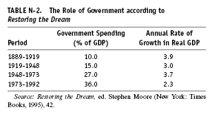
18. On this issue, see Contract with America, 125–41; Restoring the Dream, 37–52. On p. 41, the latter book has a diagram headlined “As Washington Grows, the Economy Slows.” In the diagram the percentage of the economy covered by government spending is set against the rate of growth of real gross domestic product. Table N-2 reproduces the numbers in table form. Despite the rise in the rate of growth of GDP in the third period even as government spending rose, the long-run trend is obviously an inverse one.
19. Murray Weidenbaum, “America’s New Beginning: A Program for Economic Recovery,” in Two Revolutions in Economic Policy, ed. James Tobin and Murray Weidenbaum (Cambridge: MIT Press, 1988), 294. Note that the focus is on “excessive government spending,” yet nowhere in this discussion are deficits blamed for the economy’s problems. Instead there is a prediction that deficits will decline to zero and a passing reference to the “alarming trends” of rising deficits and rising spending over the decade of the 1970s (p. 302).
20. ERP 1981; ERP 1984.
21. See Friedman, Capitalism and Freedom, as well as ERP 1982, 27–33. For a more extreme superlibertarian view, see Murray Rothbard, Power and Market, Government and the Economy (Kansas City, MO: Sheed Andrews and McMeel, 1977).
22. In 1993, economic historian Douglass C. North won the Nobel Prize in economic science for his work on how institutions interact with economic actors to make it easier or harder for economic growth to occur. One can see the proposals in the Contract with America relating to increased spending on police and prisons, increased sentences for violent criminals, and legal reform to reduce the costs to business and individuals from “frivolous” lawsuits as an effort to re-create what Republicans see is an appropriate framework within which such a market economy can function (Contract with America, 37–64, 143–55).
23. William Baumol, J. C. Panzar, and R. D. Willig, Contestable Markets and the Theory of Industry Structure (New York: Harcourt Brace Jovanovich, 1982).
24. The Contract with America devotes an entire chapter to the proposition that the Clinton administration budget cuts have weakened the defense establishment to the point where the so-called hollow military of the late 1970s is in danger of being re-created (Contract with America, 91–113). The sequel volume, Restoring the Dream, 115–18, has proposed significant privatization of federally run activities such as the Naval Petroleum Reserve, the Air Traffic Control System, and certain Amtrak routes.
25. In the 1990s, there is an effort to take this principle even further. Areas of activity previously the sole responsibility of government, such as the running of prisons, have been proposed for privatization. Private companies contract with a state government to house a certain number of prisoners, getting paid a fixed fee and making their profit by delivering the “service” to the taxpayers at a lower cost than if the state paid the costs directly. With prison building on a dramatic upsurge in the past decade and prison populations rising dramatically, this is a great new frontier for profitable activity on the part of the private sector.
26. ERP 1982, 30–31.
27. Given the incomes of all consumers, given the tastes and preference of these consumers, and given the capital and land and skills of the labor force available to be used by businesses as well as the state of technology, the satisfaction achieved by each and every consumer that is greater than or equal to the price they actually pay for what they buy exactly equals the sacrifice society has had to endure to produce the last unit of the product sold. If this occurs in every market, then this maximizes satisfaction for society as a whole. The problem of externalities is that the price paid by people does not equal the true cost to society; the satisfaction experienced by an individual does not equal the true benefit to all of society.
28. Economists would make the comparison by summing the present value of all expected net earnings of the farmer for the rest of his or her productive life. This would create what is called the capitalized value of the farmer’s income stream. In reality, such a calculation would be very uncertain, because it actually depends on how one thousand dollars, say, five years from now is discounted to create its present value. In addition, farmers may place some kind of premium on maintaining their way of life, even if the dollar value of a lifetime in farming is lower than what could be obtained by selling out to a developer. Finally, the farmer’s time horizon may include the projected incomes of his or her children and grandchildren.
29. Murray Weidenbaum, The Future of Government Regulation (New York: Anacom, 1979), 23. It should be noted that the Weidenbaum approach is not without its critics. Some have argued that his cost estimates are too high. See, for example, John E. Schwarz, America’s Hidden Success: A Reassessment of Public Policy from Kennedy to Reagan (New York: Norton, 1988), 91–98. Others have attempted to measure benefits to show that the benefits do justify the costs. See, for example, Mark Green and Norman Waitzman, Business War on the Law: An Analysis of the Benefits of Federal Health and Safety Enforcement, preface by Ralph Nader, 2d ed. (Washington, DC: Corporate Accountability Research Group, 1981). However, it is not our intention to argue these points. It is important to develop the full conservative diagnosis of what ailed the economy because the solutions proposed and attempted by both the Reagan administration and the Republican majority in Congress since 1994 aims to change public policy to meet these alleged problems.
30. Monetarists believe that the rate of growth in the money supply is the crucial determinant of the rate of growth of nominal GDP, that is, GDP uncorrected for inflation. They argue that deviations of the rate of growth of money from the current trend have a direct impact on GDP, but only after a lag of uncertain length. (They also believe that the actual division of the impact between price increases and output increases is unpredictable in the short run.) Therefore, the monetarists have argued against using discretionary changes in monetary policy to combat too much unemployment or inflation. To do so would just as likely be destabilizing as not. For a detailed monetarist historical overview, see Milton Friedman and Anna Schwartz, A Monetary History of the United States, 1867–1960 (Princeton, NJ: Princeton University Press, 1963). See also Milton Friedman, “The Role of Monetary Policy,” American Economic Review 58 (March 1968): 1–17.
31. For the original multiplier concept, see R. F. Kahn, “The Relation of Home Investment to Unemployment,” Economic Journal 41 (1931): 173–93. The marginal propensity to consume and resulting multiplier are developed in all textbooks on the principles of economics. See, for example, N. Gregory Mankiw, Principles of Economics (New York: Dryden Press, 1998), 717–18; and Joseph E. Stiglitz, Economics, 2d ed. (New York: Norton, 1997), 674–77.
32. See Friedman, Capitalism and Freedom, chap. 5, esp. p. 81.
33. Ibid., chap. 5.
34. For some examples of some of the nonsense and their common-sense refutations, see Eisner, The Misunderstood Economy, 99–103. This is not to say that there are not some potentially negative consequences should deficits and debt rise as a percentage of GDP. When that happens, the increased percentage of government revenues devoted to paying interest would reduce the ability of government to spend on other needed activities. However, most of the claims about the evils of deficit spending and the national debt focus on the “necessity” of reducing deficits to zero and “paying off” the debt. See, for example, virtually any speech by any member of Congress beginning in March 1995.
35. See A. W. Phillips, “The Relation between Unemployment and the Rate of Change of Money Wage Rates in the United Kingdom, 1861–1957,” Economica 25 (1958): 283–99.
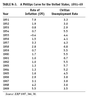
36. Table N-3 presents the unemployment rate and inflation rate between 1951 and 1969.
37. ERP 1982, 51. Table N-4 brings the Phillips Curve data from note 36 from 1970 through 1979.
38. ERP 1982, 50.
39. Within the economics profession, this view became the basis of a whole new school. Known under the general rubric of “new classical” economics, it also goes by the name of the “rational expectations” school. Very briefly, this group of economists believes that the general economy tends to an equilibrium solution and that government efforts to alter, say, the rate of growth of the economy or the level of unemployment can only have short-run impacts because in the long run, other actors in the economy will take corrective action in response to government initiatives and the economy will end up back at the same equilibrium. Thus, they strongly support the view that there is an equilibrium (“natural”) rate of unemployment toward which the economy is always tending. For a fascinating and readable analysis of this school, see Arjo Klamer, Conversations with Economists (Totowa, NJ: Rowman and Allanheld, 1984), 1–94. For criticism, see pp. 98–169. For one series of the NAIRU see Congressional Budget Office, The Economic and Budget Outlook: Fiscal Years 1998–2007 (Washington, DC: Government Printing Office, 1997), 105.

40. This may seem contradictory, but it is not. One’s marginal rate of taxation can rise even if the total percentage of one’s income paid in taxes stays the same. Consider someone with an income of $50,000 paying one rate of 10 percent in income tax. That person’s total tax is $5,000 and the marginal rate of taxation is 10 percent. Now, let us change the tax system into a two-bracket system with rates of zero percent on the first $25,000 of income and 20 percent on the second $25,000. Total taxes will still be 10 percent of income (20 percent times $25,000 = $5,000), but the marginal tax rate will have doubled. Beginning in 1964, there were a number of tax cuts that by raising personal exemptions and cutting tax rates other than the top marginal rate ended up keeping the average tax bite from rising while the marginal rate did rise.
41. It is important to understand that the tax rates shown in table 4 do not apply to the entire income of the taxpayer. Thus, someone making $25,000 in taxable income in 1980 would not owe $8,000 (32 percent of $25,000) on April 15, 1981. Instead, this person’s income tax would be the sum of the tax owed on each level of income. The first $3,400 would be tax free. The next $2,100 would be taxed at 14 percent ($294). The next $2,100 would be taxed at 16 percent ($336). Subjecting the next $17,400 to tax rates of 18, 21, 24, 28, and finally 32 percent leads to a total tax bill of $4,633. The important incentive effect of the marginal tax rate is that the extra income an individual receives as a result of making an extra effort (to take a second job, to take a higher-paying job, to make a new investment) is equal to the increase in income less the marginal tax rate. If our imaginary taxpayer with an income of $25,000 got a pay raise of $4,000, he or she would get to keep only $2,720, paying $1,280 (32 percent of $4,000) more in income tax.
42. ERP 1982, table 5-4, p. 120.
43. Assume the government raises taxes and spending by $100 billion. All of the government’s spending goes to buying military equipment, building roads, paying government employees, doing basic scientific research, thereby raising GDP. Meanwhile, some high percentage of the money paid to the government in taxes (say, $95 billion) represents a reduction in consumption expenditures, thereby lowering the GDP. But the other $5 billion in taxes paid is money that would not have been spent anyway. Thus, there is a net increase in spending of $5 billion, and that increase then is subject to the multiplier process as it ripples through the economy.
44. ERP 1982, 34–35.
45. ERP 1982, 35.
46. See, for example, Warren Shore, Social Security, the Fraud in Your Future (New York: Macmillan, 1975).
47. In 1979, 58.9 percent of the elderly would have been in poverty had they not received Social Security, unemployment compensation, and other cash payments also available universally. The other 41.1 percent with private-sector incomes above the poverty level also received Social Security. See Sheldon Danziger and Daniel Weinberg, “The Historical Record: Trends in Family Income, Inequality, and Poverty,” in Confronting Poverty: Prescriptions for Change, ed. Sheldon Danziger, Gary Sandefur, and Daniel Weinberg (Cambridge: Harvard University Press, 1994), 46.
48. Though in the case of a millionaire, the unemployment compensation and Social Security check would (today) be subject to income taxation.
49. Leonard H. Thompson, “The Social Security Reform Debate,” Journal of Economic Literature 21 (1983): 1425–67.
Chapter 4
1. This is not true about monetarism. There was a long and lively debate in 1965 around the publication of Milton Friedman and David Meiselman’s study that sought to demonstrate the superiority of “monetarist macroeconomics” as an explanation for changes in the economy to the Keynesian multiplier. See Friedman and Meiselman, “The Relative Stability of Monetary Velocity and the Investment Multiplier in the United States, 1897–1958,” in Stabilization Policies, ed. E. C. Brown (Englewood Cliffs, NJ: Commission on Money and Credit, 1963): 165–268. Friedman and Meiselman were challenged by many economists. See, for example, Albert Ando and Franco Modigliani, “The Relative Stability of Monetary Velocity and the Investment Multiplier,” American Economic Review 55 (September 1965): 693–728; and Michael DePrano and Thomas Mayer, “Tests of the Relative Importance of Autonomous Expenditures and Money,” American Economic Review 55 (September 1965): 729–51. The debate continued. See Friedman and Meiselman, “Reply to Ando and Modigliani and to DePrano and Mayer,” American Economic Review 55 (September 1965): 753–85; Ando and Modigliani “Rejoinder,” American Economic Review 55 (September 1965): 786–90; and DePrano and Mayer, “Rejoinder,” American Economic Review 55 (September 1965): 791–92.
2. For a detailed analysis that goes beyond a discussion of supply shocks to explain accelerating inflation, see Alan Blinder, Economic Policy and the Great Stagflation (New York: Academic Press, 1979). See also ERP 1978, 141.
3. Barry Bosworth, “Economic Policy,” in Setting National Priorities: Agenda for the 1980s, ed. Joseph Pechman (Washington, DC: Brookings Institution, 1980), 43. Bosworth goes on to argue, “The experience of recent recessions . . . suggests that at best an increase of 1 percent in the unemployment rate—about 1 million persons—if maintained over a two-year period would reduce inflation by only about 1 percentage point.”
4. See Blinder, Economic Policy and the Great Stagflation, 146–52. For President Ford’s two diametrically opposed requests see New York Times, October 9, 1974, 1, 24; January 14, 1975, 1, 20.
5. The government deficit as a percentage of GDP rose from less than 0.5 percent in 1974 to 3.4 percent in 1975 and 4.3 percent in 1976 (ERP 1997, 389).
6. The key barometer of Federal Reserve policy is the short-term interest rate that banks charge each other for overnight loans, the Federal Funds rate. In 1974, that rate had risen to 10.50. In 1975, the Central Bank pursued a vigorous policy to cut that rate down to 5.82, and the rate continued to fall till the first quarter of 1977 (ERP 1997, 382–83). See table W-1 on this book’s web page, <mars.wnec.edu/~econ/surrender>.
7. The GDP deflator inflation rate was 5.6 percent in 1976 and rose to 9.2 percent in 1980 (ERP 1997, 306). The consumer price index rose at a rate of 5.8 percent in 1976 to 13.5 percent in 1980 (ERP 1997, 369). See also the inflation rates in table N-4.
8. ERP 1981, 8.
9. For the budget deficit percentages, see ERP 1997, 389 (these are fiscal years). For the recession, see chap. 2, n. 21.
10. See ERP 1981, 156–58, for an explanation of the direction of fiscal policy during 1980. It is well known that Richard Nixon always believed that the Eisenhower administration’s budget surplus in 1960 and subsequent recession was the chief cause of his narrow defeat by John F. Kennedy. Too late for Nixon, the Eisenhower administration permitted the budget to move into deficit in fiscal 1961 (0.6 percent of GDP), and the Kennedy administration raised that deficit in fiscal 1962 (1.3 percent of GDP) with the enactment of the investment tax credit combined with a five-billion-dollar increase in defense purchases. We already have seen how the Ford administration dealt with the recession of 1975. In 1970 and 1971 the Nixon administration took a number of small steps to raise the amount of fiscal stimulus. (Federal deficits rose to 2.1 percent of GDP in fiscal 1971 and stayed at 2.0 percent of GDP in 1972 [ERP 1997, 389].)
11. ERP 1997, 346. See also table N-4.
12. Between 1976 and 1979, the economy created over 10 million new jobs (ERP 1997, 340).
13. This point of view is summarized by President Carter himself in his report (ERP 1981, 3–5).
14. In 1981, the Brookings Institution’s academic journal put out a special issue on the productivity slowdown. In the editors’ summary, William Brainard and George Perry noted that the causes of this phenomenon “have remained largely a mystery. In the most comprehensive study to date, Edward Denison examined seventeen alternative hypotheses and concluded that alone or in combination they could explain no more than a fraction of the slowdown” (Brookings Papers on Economic Activity 1 [1981]: vii). See also Edward Denison, Accounting for Slower Growth (Washington, DC: The Brookings Institute, 1979). Interestingly, with much more hindsight, a team of economists under the direction of William Baumol of Princeton University discovered that the slowdown in productivity of the 1970s and 1980s was actually a return to the century-long trend that had been disturbed first by a tremendous decline in growth due to the depression of the 1930s and then a tremendous increase in growth in the period between 1945 and 1972. See Jeffrey G. Williamson, “Productivity and American Leadership: A Review Article,” Journal of Economic Literature 29 (March 1991): 51–68.
15. Blinder, Hard Heads, Soft Hearts: Tough-Minded Economics for a Just Society (New York: Addison-Wesley, 1987), 24.
16. In the case of automobiles, the massive government subsidies to highway construction made automobile transportation of goods and people relatively attractive compared to rail travel and transport. There was also tremendous subsidy to housing dispersal into the suburbs with low-interest loans and tax deductions associated with home ownership. The aerospace and telecommunications industries’ dependence on government seed money and extensive research and development funds is almost self-evident. Large government purchases often become the basis of concerted business efforts to cut the cost of new technological advances. One particularly significant example is noted by the Economist.
In 1961 . . . Fairchild and Texas Instruments found themselves sitting on a clever new invention, called the integrated circuit, which nobody could afford to buy. Then, the chips cost around $120 each. By 1971, the average price was less than $42. Why the change? Mainly because President Kennedy decided to send an American to the moon—a feat which led the federal government to buy more than a million integrated circuits and taught the semiconductor industry to build them at a fraction of the initial cost. (“Will Star Wars Reward or Retard Science?” Economist, September 7, 1985, 96.)
The Internet is only the latest governm5t66666ent-created product that is now available virtually free of charge for use by the private sector.
17. The stagnation school is associated with the work of Paul Baran and Paul Sweezy in Monopoly Capital. The basic conclusion of this school is that capitalism in the twentieth century is subject to a permanent tendency for aggregate demand to fall short of potential GDP. The result is that more and more government intervention is necessary to stave off economic depressions, and even with such intervention, a tendency toward secular stagnation sets in.
This school explains the post–World War II sustained growth by stating that the massive expansion of the military during World War II had ended the depression. Then there was a short postwar consumer boom as people made up for hard times since the early 1930s. The years 1950–53 saw the Korean War, and even with the end of the war demand hardly slackened because the economy was into the suburbanization-automobilization that by the midsixties had put almost two cars in every garage and built thousands of miles of interstate highways. By the end of the 1960s, another shooting war was going on, and the economy actually pushed unemployment below the 4 percent level. With the slowdown in military spending associated with the reduction in U.S. activities in Indochina came the sluggishness of the 1970s. This was counteracted with other kinds of government spending and the creation of mountains of consumer and corporate debt, but it was not enough. The economy slipped into stagnation, and the efforts to fight it only created inflation to go along with the basic problem. For this school, the economy is successful only so long as special events, usually military spending or wars, are counteracting the basic tendency of the economy to settle into stagnation.
18. The various writers in this tradition have presented different version of this post–World War II structure (see, for example, Bowles, Gordon, and Weisskopf, After the Wasteland, 48). The text presentation is my own version based on a reading from a variety of sources as well as discussions within the Center for Popular Economics on the postwar period. The main difference between this group and the Baran-Sweezy stagnation school is that the latter sees the economy as always in danger of falling into a stagnant or worse situation absent extraordinary surges in aggregate demand. The long-swing group suggests that when a coherent structure, a social structure of accumulation, is in place, the economy generates a fairly long period of decent growth with short, mild interruptions.
19. ERP 1994, 320, 323.
20. In 1953, an American CIA operative led a joint British-American effort to overthrow the elected Iranian government, which had moved to nationalize international oil companies. That government was replaced by a monarchy headed by the shah. In 1954, the elected government of Guatemala had attempted to nationalize some of the land owned by the United Fruit Company. Under cover of protecting the hemisphere from Communist influence (the Guatemalans had bought some military equipment from Czechoslovakia), the United States again organized a coup (Bowles, Gordon, and Weisskopf, After the Wasteland, 50–51). See also Kermit Roosevelt, Countercoup: The Struggle for the Control of Iran (New York: McGraw-Hill, 1979); and Steven Schlesinger and Steven Kinzer, Bitter Fruit (Garden City, NY: Doubleday, 1982).
21. The stagnation school, by contrast, believes that the economy had just run out of causes for surges in aggregate demand, and so the natural tendency to stagnation reasserted itself.
22. Arthur Okun, Prices and Quantities: A Macroeconomic Analysis (Washington, DC: Brookings Institution, 1981), 83–126. On pp. 127–30 he analyzes the inflationary bias that collective bargaining may add to the process.
23. Gary Byner, president, Local 1112, United Auto Workers, qtd. in Studs Terkel Working (New York: Pantheon Books, 1974), 192–93.
Chapter 5
1. The rate of increase in the GDP deflator had averaged 6.3 percent in 1977 and 7.7 percent in 1978. In 1979, the first three quarters saw the annual rate of inflation rise to 8.6 percent and stay at 8.7 percent for the next two (ERP 1997, 306). Quarterly rates from Bureau of Economic Analysis, Department of Commerce.
2. ERP 1997, 422.
3. The best measure of the international value of the dollar compared to our major trading partners actually rose slightly between 1973 and 1976 before beginning to plummet (ERP 1997, 422).
4. The price of gold is per troy ounce. The monthly series for the price of gold is published by Metals Week and available from the Branch of Metals, U.S. Bureau of Mines.
5. The printout of monthly gold prices from the U.S. Bureau of Mines has the highest, lowest, and average price of a troy ounce of gold per month beginning in 1968 and continuing up to the present. Robert Bartley, quoting Roy W. Jastram, noted that “when one nation shows economic and political turbulence, its currency will decline as holders seek safe havens in other currencies. ‘But what happens when danger is sensed in every direction? There is one “currency” with no indigenous difficulties—gold. The cautionary demand for it is really a short position against all national currencies’” (Bartley, The Seven Fat Years and How to Do It Again [New York: Free Press, 1992], 109). Meanwhile, the Monthly Review, operating in the radical tradition, published an editorial identifying the spike in the price of gold as “Capitalism’s Fever Chart” (“Gold Mania: Capitalism’s Fever Chart,” Monthly Review, January 1980, 1–8).
6. ERP 1996, 280.
7. Greider, Secrets of the Temple, 109–16.
8. Greider, Secrets of the Temple, 109–23. Interestingly, in other analyses of the Fed’s policy reversal, much emphasis is placed on Volcker’s trip to an international bankers’ conference in Belgrade, Yugoslavia, which occurred after the decision of the Board of Governors but before the ratification of that decision by the Federal Open Market Committee. This has led some commentators to suggest that Volcker was responding to pressure from foreign central bankers, which of course was not true, since the decision had already been made. See, for example, Bartley, The Seven Fat Years, 85–86 and Blinder, Economic Policy and the Great Stagflation, 77.
9. “Statement by Paul A. Volcker, Chairman, Board of Governors of the Federal Reserve System, before the Joint Economic Committee of the U.S. Congress, October 17, 1979,” Federal Reserve Bulletin 65 (November 1979): 889.
10. Both nominal and real Federal Funds rates 1970–91 are collected in table W-1 at the book’s web site, <www.mars.wnec.edu/~econ/surrender>.
11. Actually, these yearly figures mask some significant variations during the year. In 1980, in particular, the rate of growth of money started out at 6.7 percent (last quarter of 1979 to first quarter of 1980) but then turned negative as the economy experienced a sharp but very short (one-quarter) recession (the rate was –3.4 percent). The shrinkage of the money supply was not, of course, what the Federal Reserve had promised when it adopted monetarism. In response, the Fed shifted to an expansionary monetary policy. The rate of growth of money shot up to 15 percent in the third quarter before subsiding to 10.9 percent in the fourth. By the first quarter of 1981, the rate of growth had fallen further to 4.6 percent. Data of the Federal Funds rate and the money supply (M1) available directly from the Board of Governors of the Federal Reserve System.
12. “Monetary Report to Congress,” Federal Reserve Bulletin 66 (March 1980): 177.
13. ERP 1994, 347. This is evidence for the charge by Greider and others that the so-called monetarist experiment was merely a political cover for interest rates high enough to wring inflation out of the economy no matter how much unemployment would be necessary. Interest rates rose high enough to get the job done, and it didn’t matter whether the growth rate of M2 or M3 slowed.
14. Beginning at 13.82 percent in January 1980, it rose to 17.61 percent in April, then fell to 9.03 percent in July (the second quarter was the time when there was a short but sharp recession), before rising to a peak of 19.08 percent in January 1981. Over the next two months it fell to 14.70 percent before rising to 19.1 percent in June. Monthly averages for the Federal Funds rate are available from the Federal Reserve Board, table J1–1. For a quarterly time series of the Federal Funds rate, see table W-1 at the web site.
15. Federal Reserve Board, table J1–1.
16. ERP 1997, 377.
17. Using annual data, both the consumer price index and the GDP implicit price deflator had the highest rate of increase in 1980 (ERP 1997, 306, 369). Using quarterly data, the first quarter of 1981 experienced the highest rate of increase in the implicit price deflator (Survey of Current Business, September 1993, 54), while for the consumer price index (urban consumers) the first quarter of 1980 experienced the highest rate of increase (Bureau of Labor Statistics, Consumer Price Index All Urban Consumers, U.S. city average 1982–84 = 100).
18. ERP 1984, 299. The prime rate is the interest rate banks charge their best business customers. The mortgage rate listed here is for a conventional mortgage with a ten-year repayment period.
19. The “true” real interest rate must somehow create a measure of the expected rate of inflation that the “average” borrower and lender have agreed upon when making the “average” loan agreement. There are a number of conventions that have been established to measure the expected rate of inflation. One of the simplest is to take the average of the preceding three years and assume that that is what borrowers and lenders expect inflation to be in the coming year(s). I have created such a table using the average inflation rate in the preceding twelve quarters for the “expected” rate of inflation in each quarter. In effect this attempts to measure what borrowers and lenders believe to be the real interest rate upon which they are agreeing. One might think of this as the planned real interest rate. To measure the actual impact on the economy of the real interest rate, I believe it is useful to concentrate on the actual burden of interest in terms of lost purchasing power. Thus, I also measure the real interest rates by subtracting the actual inflation rate in each quarter from the nominal interest rate. One might think of this as the experienced real interest rate. The inflation rate used in the appendix and throughout this book when identifying the real interest rate is the rate of increase in the GDP implicit price deflator unless otherwise noted. I choose this over the better-known consumer price index because we are looking for the generalized impact of inflation on interest rates throughout the entire economy, not just on consumers. It should be noted that no matter which way we attempt to measure real interest rates, there will always be limitations. Every individual experiences inflation differently because each person buys different types of products and “sells” different types of products, all of whose prices are changing at different rates than the average, no matter how that average is measured.
Both versions of the real interest rate peaked in 1981, fell during the recession, and then rose in 1984 as the Fed demonstrated its commitment to keeping inflation in check long before unemployment got anywhere near the 1980s version of the “natural” rate—6 percent. See tables W-2 and W-3 at the web site for details, <mars.wnec.edu/~econ/surrender>.
20. Bartley, The Seven Fat Years, 145; Greider, The Secrets of the Temple, 155–80.
21. A supply curve plots alternative prices against the quantities of the good or service businesses are willing and able to provide based on the scarcity of the resources involved. If the true scarcity of all resources used in a production process, including some, such as air and water, that aren’t bought by the producers, is accurately reflected in the costs to the businesses, we can say that the supply curve accurately measures the sacrifice made by society in producing the various quantities of that product. The demand curve plots alternative prices against the quantities of a good or service consumers are willing and able to purchase. If the true satisfaction derived by the consumer is accurately reflected in the price he/she is willing and able to pay, and if there are no spillover costs and/or benefits to noninvolved consumers, then we can say that the demand curve accurately measures the satisfaction experienced by society in consuming the various quantities of that product. Note that the “ifs” about true scarcities and absence of externalities conceal a whole host of exceptions, as even the Reagan administration’s first Council of Economic Advisers acknowledged (see pp. 39–41). For supply-and-demand curves, see any textbook on the principles of economics. For example, Mankiw, Principles of Economics, chap. 4, and Stiglitz, Economics, chap. 4, devote entire chapters to introducing these concepts.
22. A minimum wage does not permit the price to fall to its equilibrium. This deprives some of the “suppliers” (in this case workers) of the opportunity to offer their labor for sale at a wage they would be willing to accept. It also deprives some “consumers” (in this case businesses seeking to hire workers) of the ability to purchase some wage-labor at a wage they would be willing to pay. The result is an artificial reduction in the amount of labor hired and, therefore, a reduction in output. This was the major argument developed by the members of Congress, such as Majority Leader Richard Armey, himself a Ph.D. economist, against the recent increase in the minimum wage.
Table N-5 is an imagined table of alternative wages and quantities of labor offered for sale restaurants by workers and desired to be hired by businesses (the “quantity” is measured in person-hours per week). Let us assume this labor market refers to fast-food restaurants, a typical job for low-wage workers. If the minimum wage were to be set at $5.50 per hour or higher, a significant number of individuals will attempt to find work and will either be hired for fewer hours than they want or will not be hired at all. Only at the “market wage” of $5.00 an hour in this imaginary example will all workers who want to work at that wage find work. Raising that wage to $6.00 per hour would cause businesses to cut back hiring from six hundred hours a week to five hundred hours, thereby causing some people to lose their jobs. For two textbook treatments of the minimum wage, see Mankiw, Principles of Economics, 118–20, and Stiglitz, Economics, 828, 833.
23. Greider, Secrets of the Temple, 177.
24. Bartley, The Seven Fat Years, 224.
25. ERP 1982, 23.
26. “President’s News Conference on Foreign and Domestic Affairs,” New York Times, February 19, 1982, 20.
27. ERP 1982, 23.
28. ERP 1982, 109.
29. U.S. House of Representatives, Committee on Ways and Means, “Overview of Entitlement Programs,” 1993 Green Book: Data on Programs within the Jurisdiction of the Committee on Ways, and Means (Washington, DC: Government Printing Office, 1993), 1497.
30. 1993 Green Book, 1528–29.
31. See C. Eugene Steuerle, The Tax Decade: How Taxes Came to Dominate the Public Agenda (Washington, DC: Urban Institute Press, 1992), 186–87.
32. ERP 1982, 141.
33. ERP 1982, 142.
34. Paul R. Portney, “Natural Resources and the Environment: More Controversy Than Change,” in The Reagan Record, ed. John L. Palmer and Isabel V. Sawhill (Cambridge: Ballinger Publishing, 1984), 146–47.
35. To take a fairly extreme example, the Birmingham, Alabama, fire department didn’t hire its first black firefighter until 1968. A seven-year lawsuit between 1974 and 1981 finally ended with the city entering a consent decree (like a plea bargain in a civil lawsuit). To remedy the effects of past discrimination, the city agreed that if any black candidates for either appointment or promotion were qualified, all hiring and promotion would have to be split fifty-fifty between whites and blacks.
In 1983, two firefighters took the exam for lieutenant. Both passed. Under the consent decree the black firefighter got the promotion. The problem was that though both passed the exam, the white firefighter got the higher score. Right here we see one of the cores to the battle over affirmative action. By the standards of the job, both men were qualified. According to the supporters of the white firefighter, the scores on the test showed who was more qualified. The fact that there had been previous discrimination was irrelevant to the alleged injustice done to the white individual involved. From the other point of view, once the individuals involved are judged capable of doing the job, basic fairness involves permitting black candidates for jobs and/or promotion to be compensated for the disadvantages illegally imposed on people like them in the past. People who have higher test scores today are building on the ill-gotten gains of past discrimination (Thomas B. Edsall and Mary D. Edsall, Chain Reaction: The Impact of Race, Rights, and Taxes on American Politics [New York: Norton, 1992], 125–26). There is one other extremely important issue that builds strong support for affirmative action policies, even in the 1990s. That is the view that the desire to discriminate on the basis of race and gender has not disappeared just because it has been made illegal. In order to force decision makers to behave in a nondiscriminatory manner, some program needs to be in place. The victims of current discrimination cannot rely on goodwill and/or inability to cover up discriminatory behavior to protect their rights in the job market.

36. Ibid., 188.
37. Ibid., 191.
38. D. Lee Bawden and John L. Palmer, “Social Policy: Challenging the Welfare State,” in Palmer and Sawhill, The Reagan Record, 204.
39. Ibid., 205.
40. This is not the place to engage in a detailed debate about affirmative action. Two very significant affirmative action cases were decided by the Supreme Court in the late 1970s. For the legal issues and facts, see “Regents of the University of California v. Bakke,” Preview of United States Supreme Court Cases, October 1977 Term, No. 4 (September 26, 1977), 1–3; and “United States Steelworkers of America v. Weber,” “Kaiser Aluminum & Chemical Corp. v. Weber,” and “United States v. Weber,” Preview of United States Supreme Court Cases, October 1978 term, no. 31 (April 5, 1979), 1–3. The important issue is to understand that regardless of whether affirmative action programs are a good idea or not, having the chief civil-rights enforcement organizations in the country more concerned with fighting “reverse discrimination” against white people than with remedying the sorry state of affairs for black Americans sends a powerful message to those who have always resented civil-rights enforcement and the businesses who have always resented any government intrusion into how they conduct themselves.
41. ERP 1980, 118–19.
42. ERP 1982, 163–64. See also William Niskanen, Reaganomics: An Insider’s Account of the Policies and the People (New York: Oxford University Press, 1988), 119–20. Note, however, that in this book Niskanen voices some complaints about regulatory changes that were blocked. Particularly interesting is the following comment:
In 1983, the FCC proposed to relax the “financial interest and syndication rules,” which restrict the right of the TV networks to develop original programming and to syndicate reruns. These rules in effect protect Hollywood from competition by the networks. Although this proposal was broadly supported within the administration, the “California mafia” in the White House ruled in favor of Hollywood, and the proposal was withdrawn. (120)
43. In real (1987) dollars, the total regulation budget went from $4 billion in 1970 to $8.31 billion in 1981. In 1984, the number was $8.23 billion (a 1.0 percent decline) (Melinda Warren, “Mixed Message: An Analysis of the 1994 Federal Regulatory Budget,” Occasional Paper 128, Center for the Study of American Business, Washington University, St. Louis, 1994, 6).
44. 53.6 percent in 1970, 56.7 percent in 1975, 55.7 percent in 1980 (1993 Green Book, 616).
45. See ibid., 619, for the changes in the rules. For the numerical example, see p. 621.
46. Ibid., 738.
47. Ibid., 1312–13.
48. By contrast, the percentage of individuals in poverty receiving AFDC was 42.8 percent in 1975. Three years later that percentage stood at 42.4 percent (ibid., 471, 1225).
49. Ibid., 1622.
50. Ibid., 1632.
51. Table N-6 shows the participation in the food stamp program in absolute numbers and as percentages of the total population as well as the population living in poverty between 1975 and 1991.
52. Palmer and Sawhill, The Reagan Record, 370.
53. Teresa A. Coughlin, Leighton Ku, and John Holahan, Medicaid since 1980: Costs, Coverage, and the Shifting Alliance between the Federal Government and the States (Washington, DC: Urban Institute Press, 1994), 20. According to the 1993 Green Book, 1659, the per capita real dollar spending on children and AFDC adults declined from 1981 through 1984. This was at a time where other areas of Medicaid expenditure were rising in real terms, so that the overall per capita real spending rose over 9 percent.
54. Palmer and Sawhill, The Reagan Record, 370.
Since 1981, the administration has proposed more cuts in Medicaid, including an extension of reduced matching payments and a requirement that states charge beneficiaries at least a nominal amount for services received. Congress has rejected most of these proposed cuts because they would shift costs to the states or reduce service to the poor.
Note the use of the term gross national product rather than GDP. GNP differs from GDP only slightly. It adds to GDP the income Americans earn abroad and subtracts from GDP the income foreigners earn in the United States. American national income accounts shifted from GNP to GDP in 1992, so researchers who wrote before then used gross national product as their measure of total national output.

55. Robert B. Carlson and Kevin R. Hopkins, “Whose Responsibility Is Social Responsibility?” Public Welfare 39 (fall 1981): 10, qtd. in Bawden and Palmer, “Social Policy,” 192n. This rather vague definition obscures a centuries-long debate as to who constitutes the “truly needy.” For a historical survey, see Richard A. Cloward and Frances Fox Piven, “The Historical Sources of the Contemporary Relief Debate,” in Fred Block, Richard A. Cloward, Barbara Ehren-reich and Frances Fox Piven, The Mean Season: The Attack on the Welfare State (New York: Pantheon Books, 1987), 3–43. In practice, since the beginning of the Reagan administration “truly needy” has come to refer to people who are not physically or mentally able to work.
56. 1993 Green Book, 867.
57. Ibid., 836–37.
58. Bawden and Palmer, “Social Policy,” 201.
59. 1993 Green Book, 66.
60. Ibid., 70.
61. The percentage of unemployed workers receiving compensation averaged 50 percent in 1974, 76 percent in 1975, and 67 percent in 1976, the first full year of recovery (ibid., 491).
62. The percentages in 1981 and 1983 were 41 and 44 percent respectively (ibid., 491).
63. In addition to the explicit changes in federal government policy, there were a number of changes adopted that encouraged states to tighten eligibility. For details, see Marc Baldwin and Richard McHugh, “Unprepared for Recession: The Erosion of State Unemployment Insurance Coverage Fostered by Public Policy in the 1980s,” Briefing Paper, Economy Policy Institute, 1992, esp. 4–7.
64. See ERP 1982, 33–34, for an analysis of why government “insurance” against low or no income is necessary because private-sector insurance will always leave some group uninsured as “bad risks.”
65. Martin Feldstein, “Social Security, Induced Retirement and Aggregate Accumulation,” Journal of Political Economy 82 (1974): 905–25. See in rebuttal Dean Leimer and Selig Lesnoy, “Social Security and Private Saving: New Time-Series Evidence,” Journal of Political Economy 90 (1982): 606–29; and Robert Eisner, “Social Security, Saving, and Macroeconomics,” Journal of Macroeconomics 5 (1983): 1–19.
66. David Stockman, The Triumph of Politics: Why the Reagan Revolution Failed (New York: Harper and Row, 1986), 181–93. See also Niskanen, Reaganomics, 37–38.
67. 1993 Green Book, 30–35. According to estimates from 1994, the retirement trust fund of the Social Security system will begin running deficits in 2015 and will have absorbed all of the built-up surplus by the year 2036 (C. Eugene Steuerle and Jon M. Bakija, Reforming Social Security for the 21st Century [Washington, DC: Urban Institute Press, 1994], 51). These estimates change with every report from the trustees of the Social Security system. More recent reports place the year when deficits will begin earlier and the exhaustion of the surpluses significantly earlier than 2036.
68. Bawden and Palmer, “Social Policy,” 191.
69. Steuerle and Bakija, Reforming Social Security, 237.
70. For the Medicare spending, see 1996 Green Book, 133–34. For Social Security spending and total federal spending see ERP 1997, 391, 389. (Once again, these are fiscal years.)
71. Bawden and Palmer, “Social Policy,” 191. For details, see 1993 Green Book, 147–48. Note that the data presented in the table on p. 235 in the 1996 Green Book is clearly in error. A spending reduction of less than one-half billion dollars resulting from the change in hospital reimbursement is much too low. Similarly, the changes from the 1982 Tax Equity and Fiscal Responsibility Act described on pp. 223–25 could not have ended up reducing expenditures by $23 billion between 1983 and 1987, in part because the changes in the 1983 bill superseded the hospital reimbursement changes in the 1982 act.
72. For calendar years 1980–83, the actual level of intergovernmental grants was $88.7, $87.9, $83.9, $87.0. Note that this is in a context of a rising overall federal budget (ERP 1994, 365). By contrast, such grants rose in absolute terms in both 1974 and 1975 (ERP 1980, 289).
73. George E. Peterson, “Federalism and the States: An Experiment in Decentralization,” in Palmer and Sawhill, The Reagan Record, 219–20.
74. Ibid., 224.
75. Table N-7 shows the relationship of individual and corporate income tax receipts to gross domestic product from 1979 to 1985. Ignoring the recession years of 1981 and 1982 and the first recovery year of 1983, even in 1984 and 1985, the ratio of income tax collections to GDP had remained a full percentage point lower than in 1978 and 1980 and one and a half percent lower than in 1979.
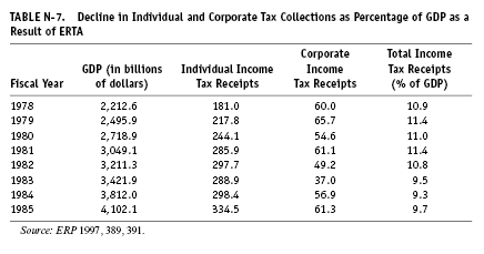
Chapter 6
1. ERP 1997, 389. Recall (see above, pp. 23–24) that the absolute level of the budget deficit does not tell us anything about its impact on aggregate demand. For that we need to express it as a percentage of GDP.
2. As noted in note 54 to the previous chapter, the Department of Commerce switched from gross national product to gross domestic product for their measurement of total economic activity. However, the Bureau of Economic Analysis tables for the fixed-unemployment GNP have not been so transformed.
3. Data supplied by the Bureau of Economic Analysis, Government Division, Department of Commerce, calculations by Michael Webb. The calculation is based on government expenditures and revenues calculated using the rules of payments and taxation and applying those rules to the estimated GNP with 6 percent unemployment. The structural deficit so calculated continued to rise through 1985. See table W-1 at this book’s data web site, <mars.wnec.edu/~econ/surrender>.
4. Though we are here focusing on the federal deficit, it is important to note that the actual impact on aggregate demand is created by the total government deficit (or surplus). In table W-1 at the web site, a series of the total government deficit/surplus as a percentage of GDP is included along with the structural deficit as a percentage of gross national product.
5. Monthly money stock information is available from the Federal Reserve Board. See table W-1 at the web site for quarterly data on the rate of growth of M1.
6. This is not, of course, how the strong defenders of the incentive policies of the Reagan administration see it.
With the Phillips curve, the Keynesians found themselves trying to hit two birds [inflation and unemployment] with one stone. To fight inflation, you needed one lever. And to fight stagflation, you need a second one. . . . the answer was clear: You fight inflation with monetary policy. . . . And you fight stagnation, you stimulate the economy, with incentive-directed tax cuts. (Bartley, The Seven Fat Years, 59)
7. I don’t want to be misunderstood. I personally believe that the pain and suffering inflicted on people during a recession is a terrible blot on our economic system. For some impressionistic details, see Greider, Secrets of the Temple, 450–71. The reason I choose not to belabor this issue is that from the point of view of long-run policy, the success or failure of the Reagan-Volcker program is to be judged not by the existence of the recession but by the nature of the recovery. Those are the terms on which the architects of the policy wished to be judged, and those are the terms on which history must make the judgment.
8. See Isabel V. Sawhill and Charles F. Stone, “The Economy, the Key to Success,” in Palmer and Sawhill, The Reagan Record, 82–90, for some simulations of how a different policy mix might have avoided the depth and severity of the recession and still brought inflation down (though not as far down as actual policy). See also Blinder, Hard Heads, Soft Hearts, 79.
9. For details of this point of view, see Bowles, Gordon, and Weisskopf, After the Wasteland, 80–96.
10. This concept is explained fully in the useful textbook Understanding Capitalism, by Samuel Bowles and Richard Edwards (New York: Harper Collins, 1993), 433–39.
11. See, for example, Bowles, Gordon, and Weisskopf, After the Wasteland, 187–233.
12. For example, in his account of the Reagan years Robert Bartley of the Wall Street Journal argued that the recession was caused by a failure to concentrate the supply-side incentives in the first year of the Economic Recovery Tax Act, coupled with the Federal Reserve’s inconsistent monetary policy. Bartley would have preferred a “commodity” standard to anchor the value of the dollar rather than the restrictive monetary policies of Volcker’s Fed. See Bartley, The Seven Fat Years, 103–33.
13. For example, despite the very low unemployment rates in 1967 and 1968, the federal deficit as a percentage of GDP only reached 2.9 percent in fiscal 1968. See ERP 1997, 390.
14. If we are interested in the impact of policy, the structural deficit of the federal government is important. However, if we want to observe the impact on aggregate demand, we have to observe the actual deficit of all levels of government, federal, state, and local. Thus, in table W-1 at the web site we have tracked the total government deficit as a percentage of GDP.
15. These are calculations of the after-the-fact real interest rate. The real rate generated with a series of expected rates of inflation shows a similar qualitative difference in general between the post-1983 years and the period of the 1970s, but it does experience high levels in both 1970 (averaging 3.23 percent) and 1974 (averaging 5.03 percent). The rate of growth of the money supply tells a different story. Except for 1984, the rate of growth of M1 was quite high from the abandonment of monetarism in the last quarter of 1982 through 1986. Beginning in 1987, the Fed tightened up on the rate of growth of money. What is interesting is that through most of the decade of the 1980s, the impact of the rate of growth of money on the real interest rate and on the rate of growth of nominal GDP was hard to identify. For quarterly details, see table W-1 at the web site, <mars.wnec.edu/~econ/surrender>, for the rate of growth of M1 and the after-the-fact measure of the real interest rate. Tables W-2 and W-3 at the web site have two measures of the expectations-generated real interest rate.
16. Congressional Budget Office, Defense Spending and the Economy (Washington, DC: Government Printing Office, February, 1983), 35–36.
17. This decision and the White House and bond market reactions are reported in Greider, Secrets of the Temple, 611–24.
18. (ERP 1986, 292). Note that these figures are percentages of the entire labor force and are therefore not completely comparable to the figures in table W-4 on the web site because those figures are for the civilian labor force only.
19. Steuerle, The Tax Decade, 42.
20. Ibid., 186. For GDP, see ERP 1997, 300.
21. Steuerle, The Tax Decade, 186. For details see pp. 58–61.
22. Interestingly, Steuerle argues that part of the reason those first efforts failed was not merely that Social Security had a strong and politically potent constituency.
During 1981, the administration held some internal meetings on Social Security reform: with some political officials from the White House, the Department of Health and Human Services and the Social Security Administration. In attendance were many new political appointees with strong but sometimes unchecked views on what was wrong with the system. The newcomers were so distrustful of the entire civil service that they prevented many of the most talented individuals in the executive branch, including top analysts from the Social Security Administration, from attending these meetings. Valuable information was thereby precluded through inadequate use of staff. The controversy that surrounded the proposals that were tentatively released, therefore, was due not simply to the difficulty and sacredness of the Social Security issue; it was also due to bad planning and the forwarding of some poorly designed proposals. (The Tax Decade, 62)
23. This last item ultimately reduced payments by $39.4 billion between 1983 and 1989. This may seem strange because it is only a onetime delay. However, if there had been no delay, the cost-of-living increase would have been paid six months early every year after 1983 as well. Thus, the total cost of the delay to the recipients (and thus the savings to the Social Security trust funds) adds up year after year. See 1993 Green Book, 34. See also Steuerle, The Tax Decade, 62–63.
24. See 1993 Green Book, 30–31, for data and some numerical examples.
25. John H. Makin and Norman J. Ornstein, Debt and Taxes (New York: Times Books, Random House, 1994), 222–23.
26. 1993 Green Book, 34. Focusing only on tax increases, not benefit changes, Steuerle comes up with the number $110.5 billion (The Tax Decade, 65). Steuerle’s total is approximately $20 billion lower than the 1993 Green Book’s figure, but since he used the 1990 Green Book, I assume the figure in the text to be more accurate.
27. See Steuerle, The Tax Decade, 49, for an example of how a 9 percent real loss on an investment could translate into a positive profit of 3 percent for a taxpayer who borrowed the money, depreciated the asset at the accelerated post-1981 rate, and took the investment tax credit. Steuerle also notes that by 1984
“tax straddles” . . . had become too popular for the legislature to ignore anymore. A person could essentially buy and sell rights to future commodities in a way that created equal gains and losses—like flipping a coin and betting on both heads and tails. The taxpayer would then take losses on whichever “leg” of the straddle generated a loss, use that loss to offset other capital gains that otherwise would be taxable, and then defer recognition of the “leg” with a gain to future years. (67)
28. Ibid., 92.
29. Ibid., 186.
30. Ibid., 112.
31. Ibid., 122.
32. The effective rate of taxation is defined as the ratio of actual taxes paid to the broadly defined tax base (ignoring preferences for the moment). Recall that the rate of inflation changes the real value of the depreciation allowances as well as the real value of interest deductions. (See ibid., 151, for some alternative calculations at different inflation rates.) Other variations in effective tax rates have to do with whether or not the particular industry devotes most of its investment dollars to equipment purchases that would then trigger the investment tax credit.
33. Under pre-1986 law, the capital-gains exclusion would have made only forty thousand dollars taxable, in this case overcorrecting for inflation.
34. Steuerle, The Tax Decade, 145
35. Bartley, The Seven Fat Years, 157.
36. The original idea of the Tax Reform Act was to have two positive rates as well as a “zero bracket.” These rates ended up being 15 percent and 28 percent. However, to raise more revenue, at a certain level of income (seventy thousand dollars in 1987, thereafter indexed for inflation), the benefits of the zero bracket and lower rate of 15 percent were phased out at the rate of 5 percent of income over that threshold. This had the effect of raising the marginal tax rate temporarily to 33 percent until all the benefits of the zero bracket and 15 percent rate had disappeared. At that point (in 1987 at an income of $127,000, thereafter indexed) the marginal tax rate reverted to 28 percent.
37. This changed the definition of “long-term” capital gains from one year to a year and a half. Allegedly this was designed to reduce the tax advantage for purely speculative investments—to give the preference to those making some kind of a “commitment” to their investments. See “Highlights of Some Provisions Covering Taxes and Tax Credits, Capital Gains,” New York Times, July 30, 1997, A16.
38. Murray Weidenbaum, Rendezvous with Reality: The American Economy after Reagan (New York: Basic Books, 1988), 9.
39. Niskanen, Reaganomics, 125.
40. Real spending levels were $8.23 billion in 1984, $8.42 billion in 1985, $8.23 billion in 1986, $8.99 billion in 1987, $9.56 billion in 1988, and $9.73 billion in 1989 (Warren, “Mixed Message,” 25).
41. Coughlin, Ku, and Holahan, Medicaid since 1980, 104.
42. ERP 1989, 196.
43. ERP 1989, 198.
44. Contract with America, 135. See also the arguments on pp. 139–41.
45. See p. 207 and pp. 212–14 for a discussion of the Bush administration’s activities in this area.
46. In the first four months under the 1984 law, the AFDC grant would be cut 43 cents for every dollar of earnings. During the next eight months, the benefit reduction rate climbs to 63 cents out of every dollar. This is lower than the cut under OBRA, 1981, but it is still high enough to reduce the monthly cash grant in the median state to zero. After twelve months on welfare, the grant is reduced by approximately 70 cents for every dollar of earnings. Under the 1988 law, each of these rates is slightly reduced. The numbers are 36, 62, and 67 cents per dollar of benefits for the same three durations. Again, after four months the net benefits in the median state have been reduced to zero (1993 Green Book, 621).
47. Ibid., 625. See pp. 630–33 for details on which states offered which programs as of 1993. For participation requirements, see pp. 627–28.
48. Ibid., 640–44.
49. Ibid., 668.
50. 1996 Green Book, 467.
51. 1993 Green Book, 688.
52. Table N-8 shows the percentages for 1984 through 1990.
53. Gary Burtless, “Effects on Labor Supply,” in The Economic Legacy of the Reagan Years: Euphoria or Chaos? ed. Anandi Sahu and Ronald Tracy (New York: Praeger, 1991), 58. The data is collected in a table on p. 57.
54. Contract with America, 65–77. See also Restoring the Dream, 53, 163–72.
55. For the trend in the poverty threshold for different-sized families, see 1993 Green Book, 1310. By 1989, the three-person family needed $9,885 per year to escape from poverty, over 40 percent above the income of a year-round, full-time worker receiving minimum wage.
56. Ibid., 1630: “The across-the-board benefit increase in maximum benefits (above normal inflation adjustments) called for by the act was 0.65 percent in fiscal year 1989, 2.05 percent in fiscal year 1990, and 3 percent in later years.”
57. For data on enrollment and expenditures by eligibility groups, see Coughlin, Ku, and Holahan, Medicaid since 1980, 20–21.
58. Ibid., 35.
59. Ibid., 46–53.
60. Ibid., 58–59.
61. For details see 1993 Green Book, 261–62, especially the footnote on p. 261.
62. See Coughlin, Ku, and Holahan, Medicaid since 1980, 105.
63. Medicaid was $78.2 billion in 1990. National spending on nursing-home care was $53.3, of which approximately 47 percent was paid by Medicaid (1993 Green Book, 266, 1647, and 259). Elsewhere the Green Book gives a percentage of 27 percent of Medicaid spending for fiscal 1991. This is lower than the figure in the text because it excludes nursing homes for the retarded. Whatever the percentage, the following information is quite relevant: “In 1991, Medicaid nursing home payments amounted to 60 per cent of total Medicaid payments for all services for all elderly beneficiaries” (ibid., 261).
64. For the Medicare spending, see 1996 Green Book, 134. For Social Security spending and total federal spending see ERP 1997, 391, 389.
65. This result was obtained by comparing the average annual benefit per aged person in 1980 and 1990 (1993 Green Book, 138) and deflating both numbers by the consumer price index (ERP 1995, 341). The more rapid escalation in the costs of Part B should not be surprising, since hospital reimbursements had been subject to a form of price controls since 1983. This result also demonstrates one of the problems health care policymakers began to discover during the 1980s: price controls in one part of the system merely encourages price to rise all that more rapidly in other parts of the system. If we deflate the average annual benefit per aged person by the consumer price index for medical care, the real benefits still have risen, but by less than 10 percent for Medicare Part A and a bit less than 80 percent for Part B. This demonstrates that the rising price of medical care was not the only reason for increased spending, that there was an increase in the real amount of services delivered. Again, the difference between Part A cost increases and Part B relates to the imposition of price controls.
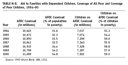
66. See 1993 Green Book, 266.
67. In Restoring the Dream, 133—40, the Republican members of the House of Representatives describe how they will save Medicare from bankruptcy and offer senior citizens more choice than they now have while avoiding coercing Medicare beneficiaries “into mandatory health alliances such as those proposed in Clinton’s 1994 health-care proposal.” They do this without proposing any comprehensive health care reform, and in fact they imply that such a reform is unnecessary because “Market-based reforms have reduced the inflation rate in private-sector spending to 4.7 percent” (139). Republicans and Democrats did cooperate in passing a very modest health reform bill, the Kennedy-Kassebaum Act of 1996.
68. Robert Pear, “$24 Billion Would Be Set Aside for Medical Care for Children,” New York Times, July 30, 1997, A17. This change would permit states to extend insurance to over 2 million previously uncovered children and retain coverage to over 1 million who would have lost Medicaid coverage as a result of the welfare law changes. See O’Neill, letter to Raines, 48–50.
69. 1993 Green Book, 491.
70. Blinder, Hard Head, Soft Hearts, 103.
71. Ibid., 221n. 41.
72. Blinder claims that this occurred because of “accounting gimmicks and budget trickery that gave the appearance of compliance with Gramm-Rudman without the reality” (ibid., 104).
73. Automatic reductions occurred only if the budget as adopted projected a deficit $10 billion above the target set by the law during the first two weeks. An incorrect projection does not trigger the automatic cuts when it is proven wrong later in the fiscal year (ERP 1990, 70; see also Blinder, Hard Heads, Soft Hearts, 104).
74. “[I]f the projected deficit exceeds the target by more than [$10 billion] the Administration calculates automatic spending cuts (or sequester) needed in each program to meet the . . . deficit target. If legislation does not achieve this reduction by the end of the second week of the fiscal year, the President orders a sequester” (ERP 1990, 71).
75. Whereas the 1990 report of the president’s Council of Economic Advisers described the workings of the Gramm-Rudman-Hollings Act (pp. 69–73), the 1991 report doesn’t even mention it, focusing instead on the OBRA of November, 1990 (ERP 1991, 46–49).
76. It is important to note, however, that the Reagan administration made no moves toward a more competitive international trade stance. Despite the rhetoric of conservative economics in favor of “free trade,” the administration supported the profitability of the top American industries, particularly the automobile industry, “presid[ing] over the greatest swing toward protectionism since the 1930s” (Shafiqul Islam, “Capitalism in Conflict,” Foreign Affairs 69 (1990): 174). This judgment, which is echoed by the work of Patrick Low in Trading Free (New York: Twentieth Century Fund, 1993), 271, 270ff., is consistent with the view that the real role for government in our kind of society is to rig the market in favor of those who already have an advantage and that the “principles” of conservative economics that we identified in chapter 3 and that we have used as yardsticks for the Reagan administration’s policy initiatives are routinely ignored whenever it serves the higher purpose of increasing the wealth and power of the already wealthy and powerful. Though I find significant evidence for this general point of view, I reiterate that the analysis of this book reaches a different conclusion. Whatever the motivations of policymakers and their intellectual supporters, the changes identified in the previous two chapters do constitute a qualitative shift in the role of government in the American economy. In addition, as we will see in the following chapters, despite the increase in protectionism, U.S. industry was subjected to increased international competitive pressure throughout the two Reagan terms.
Chapter 7
1. “The Real Reagan Record,” National Review, August 31, 1992, 25–62.
2. Bartley, The Seven Fat Years, 141–42.
3. Jeffrey Davis and Kenneth Lehn, “Securities Regulation during the Reagan Administration: Corporate Takeovers and the 1987 Stock Market Crash,” in Sahu and Tracy, Economic Legacy of Reagan, 8.
4. “Who Business Bosses Hate Most,” Fortune, December 4, 1989, 107, qtd. in Bartley, The Seven Fat Years, 140.
5. Bartley, The Seven Fat Years, 140.
6. ERP 1985, 187–89. There remains a significant debate as to the long-run consequences for the actual productivity of firms that are successfully targeted for takeover. Compare Davis and Lehn, “Securities Regulation,” 131–34, with Robert T. Kleiman, “‘Securities Regulation during the Reagan Administration’: Comment,” in Sahu and Tracy, Economic Legacy of Reagan, 141–42. See also William F. Long and David J. Ravenscraft, “Lessons from LBOs in the 1980s,” in The Deal Decade: What Takeovers and Leveraged Buyouts Mean for Corporate Governance, ed. Margaret M. Blair (Washington, DC: Brookings Institution, 1993), 222–24.
7. ERP 1989, 39. Note again the reference to gross national product rather than GDP.
8. ERP 1989, 56–57.
9. ERP 1989, 62.
10. Note this differs from the depreciation businesses are permitted to deduct from taxable income. The government-measured capital consumption allowance is based on fixed service lives for each type of capital equipment in use and is measured by deducting the total value of the investment divided by that service life every year.
11. The unemployment rate fell from 9.4 percent in the third quarter of 1983 to 7.5 percent in the second quarter of 1984 (U.S. Department of Labor, Bureau of Labor Statistics, Current Population Survey). Real GDP per capita grew at the rates of 7.9 percent, 6.1 percent, 6.3 percent, 8.1 percent, and 5.2 percent from the second quarter of 1983 through the second quarter of 1984. Investment as a percentage of GDP rose from 14.3 percent in the first quarter of 1983 to 16.6 percent in the third quarter of 1984 (U.S. Department of Commerce, Bureau of Economic Analysis). For all the quarterly numbers, see table W-4 at the web site, <mars.wnec.edu/~econ/surrender>.
12. ERP 1997, 390.
13. For the quarterly Federal Funds rate, see table W-1 on the web site. Monthly rates available from the Federal Reserve Board, FFR, effective rate averages of daily figures, October 4, 1994, table J1–1 (monthly values of FFR 1964–September 1994). For the capacity utilization rate and unemployment rate, see table W-4 on the web site.
14. ERP 1989, 109.
15. ERP 1996, 280–81. It is also important to note that during this period, the macroeconomic policies pursued by our major trading partners, particularly West Germany and Japan, were much less expansionary. For details, see Robert Blecker, Beyond the Twin Deficits: A Trade Strategy for the 1990s (Armonk, NY: M. E. Sharpe, 1992), 37–40, especially the table on p. 39.
16. As Benjamin Friedman writes,
The chief counterpart of our overconsumption in the 1980s has been underinvestment. On average during the prior three decades, we invested 3.3 percent of our total income in net additions to the stock of business plant and equipment. . . . Thus far [1987] during the 1980s, the average has been just 2.3 percent. (Day of Reckoning: The Consequences of Economic Policy under Reagan and After [New York: Random House, 1988], 28–29).
Note, however, that this decline in net investment is not matched completely by a decline in gross investment. See table 12.
17. ERP 1990, 70–71.
18. Friedman, Day of Reckoning, 174.
19. See table 11 for evidence as to whether or not this was in fact true.
20. “This idea of permanent or irreversible effects of a temporary exchange rate changes has become known as “hysteresis” . . . temporary but large appreciation of a nation’s currency induces foreign firms to enter the domestic market as long as they can still make a profit over their operating costs in their own currency in spite of the home currency’s depreciation. Thus the market structure of the home country is permanently altered” (Blecker, Beyond the Twin Deficits, 48). For a detailed model see Richard E. Baldwin, “Hysteresis in Import Prices: The Beachhead Effect,” American Economic Review 78 (September 1988): 773–85.
21. Blecker, Beyond the Twin Deficits, 49.
22. See Friedman, Day of Reckoning; Peter Peterson, “The Morning After,” Atlantic Monthly, 260 (October 1987): 43–69; Alice Rivlin, ed., Economic Choices, 1984 (Washington, DC: Brookings Institution, 1984); and Henry J. Aaron et al., Economic Choices, 1987 (Washington, DC: Brookings Institution, 1986).
23. The Federal Funds rate averaged below 7 percent in 1986 and 1987; the rate of growth of M1 went from a low of 5.7 percent in 1984 to 12.4 percent and 17 percent in 1985 and 1986 respectively before falling back to 3.5 percent in 1987. For the Federal Funds rate see Federal Reserve Board, table J1–1, available from the Federal Reserve Board. For the rate of growth of M1 see ERP 1989, 385. The real Federal Funds rate, though remaining at a historically high rate, did fall below 3 percent for two quarters in 1986 and the first quarter of 1987.
24. ERP 1994, 241.
25. In 1980, the merchandise trade deficit was 0.9 percent of GDP, while the 1992 deficit was 1.5 percent of GDP (ERP 1996, 392, 280). The full balance on current account (which is the usual statistic reported in the press as the “trade deficit”) went from surplus in 1980 to a deficit of close to 1 percent of GDP.
26. Economists say you are “receiving” an “implicit income”—the rent you do not have to pay because you own your own home. It is not as outrageous as it sounds. When you live in a house or apartment you are “consuming” the services of that structure, whether you pay rent or not.
27. Friedman, Day of Reckoning, 151.
28. ERP 1996, 280.
29. Friedman, Day of Reckoning, 64–67. Some examples from Friedman: “In 1984 Nestle . . . paid $3 billion to buy Carnation. In 1986 Unilever . . . paid $3 billion for Chesebrough-Pond’s, and Hoechst . . . paid $2.8 billion for Celanese. In 1988 Bridgestone . . . paid $2.6 billion for Firestone” (66).
30. Robert Reich, The Work of Nations: Preparing Ourselves for 21st Century Capitalism (New York: Knopf, 1991), 136–68.
31. An exception is the serious but critical study of modern radical analyses of imperialism by Benjamin J. Cohen, The Question of Imperialism (New York: Basic Books, 1973). For his discussion of whether poor countries are exploited by foreign domination, see pp. 145–227.
32. Friedman, Day of Reckoning, 76.
33. Ibid., 79–80.
34. Bowles, Gordon, and Weisskopf, After the Wasteland, 123–31.
35. Ibid., 159.
36. Robert Pollin, “Budget Deficits and the US Economy: Considerations in a Heilbronerian Mode,” in Economics as Worldly Philosophy: Essays in Political and Historical Economics in Honour of Robert L. Heilbroner, ed. Chatha Blackwell and Nell Blackwell (New York: St. Martin’s, 1993), 128.
37. Ibid. This is what Pollin calls “necessitous” demand for credit. See Robert Pollin, “The Growth of US Household Debt: Demand-Side Influences,” Journal of Macroeconomics (spring 1988): 231–48.
38. Pollin, “Budget Deficits,” 130.
39. “In earlier historical phases, the rise of private debt financing was checked and reversed when credit bubbles were burst by severe debt deflations and widespread defaults, which in turn forced the economy’s aggregate rate of debt financing sharply downward. In the contemporary period, cyclical deficits counteract the debt deflation process by increasing the level of aggregate income in the short run” (ibid., 133).
40. Michael Perelman, The Pathology of the American Economy (London: Macmillan, 1993), 6–7.
41. Ibid., 9.
42. Pollin, “Budget Deficits,” 133.
43. See pp. 70–72.
44. See pp. 138–39.
45. This structure is termed the “underlying power of capital” and developed and measured in Samuel Bowles, David M. Gordon, and Thomas Weisskopf, “Business Ascendancy and Economic Impasse: A Structural Retrospective on Conservative Economics, 1979–1987,” Journal of Economic Perspectives 1989 (winter): 107–33. See especially the table on p. 117 and pp. 122–30.
46. The job satisfaction index is derived from polls conducted by the Opinion Research Corporation. Bowles, Gordon, and Weisskopf counted the percentage of employees who answered the question “How do you like your job—the kind of work you do?” with either “Very much” or “A good deal” (Bowles, Gordon, and Weisskopf, After the Wasteland, 102).
47. This is a measure that takes the gross hourly wage of nonsupervisory workers, adds the fringe benefit of medical insurance, and subtracts Social Security and personal income taxes. See Thomas Weisskopf, “Use of Hourly Earnings Proposed to Revive Spendable Earnings Series,” Monthly Labor Review, November 1984, 38–43.
48. Bowles, Gordon, and Weisskopf, After the Wasteland, 102.
49. F. W. Taylor developed a system he called “scientific management” in the early years of the twentieth century. He urged business leaders to recognize that initially the workers monopolized the knowledge of the production process and, following their obvious self-interest, attempted to make the job as easy as possible for themselves. Taylor started by studying the processes and then attempted to force the workers to work harder. He had an extraordinarily difficult time but ultimately succeeded in the experiments he carried out. This whole process is described in great detail in Taylor’s autobiographical works. See, for example, F. M. Taylor, The Principles of Scientific Management (New York: Harper and Brothers, 1916), 42–52.
50. See p. 67.
51. See Bowles, Gordon, and Weisskopf, After the Wasteland, 126, for a particularly dramatic illustration. Union membership was above 20 percent of the workforce and had fallen to 15 percent by the end of the decade.
52. The point is, I would fear being fired from a job that paid me what I considered a good wage more than I would fear being fired from a job that paid me what I considered a very low wage. If I were in a job in which I got no raise over a five-year period during which inflation had eroded some of my real purchasing power, my attitude toward my job would undoubtedly decline.
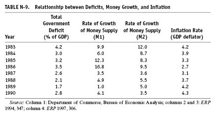
53. Milton Friedman and Rose Friedman, Inflation: Causes and Consequences (New York: Asia Publishing House, 1963), 17.
54. Table N-9 gives annual information on deficits, money supply growth, and inflation. As deficits fell as a percentage of GDP, the rate of growth of money (both the broader and the narrower measure) tended downward as well. In the two years when the trend was reversed (1985 and 1986) the rate of growth of money increased as well. But the rate of inflation continued to trend downward during those two years of rising deficits and rising rate of money growth, and when the deficit increase and money growth reversed themselves between 1986 and 1989, the rate of growth of inflation began to increase.
Chapter 8
1. The profit rate in the nonfarm business sector averaged 4.1 percent between 1980 and 1988, reaching 4.6 percent in 1988. This is in contrast to the 1974–79 period, when the profit rate averaged 2.42 percent and reached 2.94 percent in 1979. See Baker, “Trends in Corporate Profitability,” tables 6 and 7. The after-tax profit rate of nonfinancial corporations rose from 4.26 percent in 1974–79 to 4.75 percent in 1980–88, reaching 5.82 percent in 1988 (see ibid., tables 1 and 2).
2. Tables W-4 and W-5 at the web site, <mars.wnec.edu/~econ/surrender>, provide the quarterly data from 1960 through 1991. The raw data for table W-4 is summarized in table 12, the appendix to this chapter.
3. We should remember that in this discussion we are using the term investment in the same way we introduced it in chapter 2: as a real, tangible, creation of a capital asset. In the National Income and Product Accounts of the United States it is called Gross Private Domestic Investment and includes all construction of new structures, all new business equipment, and net additions to business inventories. We will discuss the potential roles of purely financial investments (such as business merger activities, the buying and selling of corporate stocks and bonds) on pp. 156–57.
4. ERP 1986, 288; ERP 1994, 307.
5. Investment as a percentage of GDP actually averaged 17.1 percent for the six quarters following the peak in the first quarter of 1980. For the next six quarters (five of which constituted the recession of 1981–82), investment as a percentage of GDP averaged 15.6.
6. Steuerle, Taxes, Loans, and Inflation, 29.
7. Steuerle, The Tax Decade, 24–25.
8. Though the National Bureau of Economic Research identified the third quarter of 1973 as a peak and the third quarter of 1981 as a peak, the 1981 peak was the result of a very short and not very dynamic recovery from the equally short recession of 1980, which actually only lasted one quarter. The unemployment rate at the peak in 1973 was 4.8 percent and the capacity utilization rate 88.5 percent, while the unemployment rate at the 1981 peak was 7.4 percent and the capacity utilization rate 81.6 percent. These were hardly improvements over the trough values for 1980 of 7.7 percent unemployment and 80.0 percent of capacity utilization. Thus, a peak-to-peak comparison of 1973 to 1981 is very misleading. Either one should use the period from the peak of 1973 to the peak of 1980, or as we do in the text, take the longer periods from 1969 to 1980 or 1970 to 1982.
9. It is important at this point to recognize that these average rates of productivity growth are not the same as the compound rate of growth. Let me illustrate. If over a ten-year period, productivity grows 10 percent, the average is 1 percent per year. But the compound rate of growth is actually a bit less (0.96 percent). Thus, for any given change over a period of years, the cumulative compound rate is always lower than the average rate. If we try to compare productivity growth over different length periods of time, the longer the period, the lower the relationship between the compound rate and the average rate. So if productivity were to grow 20 percent over two years, the average would be the same as for a 10 percent growth over ten years, but the compound rate would be lower (0.92 percent). Thus, the appropriate comparison for productivity growth over different length periods of time is the average per period rather than the cumulative compound rate. This same principle applies to the rate of growth of per capita GDP.
10. See Robert Kuttner, Everything for Sale: The Virtues and Limits of Markets (New York: Knopf, 1996), 178–88, and especially his argument that
the claim that target firms are poorly managed underperformers is not borne out by the facts. . . . Many of the takeovers, in hindsight, turned out to be bad deals. . . . There is a long catalogue of cases in which the acquiring firm . . . knew less about what it was buying than the established management, and proved to be an even worse manager. Several recent studies confirm that hostile takeovers . . . tend to depress the performance of the raiding firm. (183–84)
11. Division of Productivity Research, Office of Productivity and Technology, Bureau of Labor Statistics, “Computer Printout of Industry Analytical Ratios for the Business Sector, All Persons” (available from Bureau of Labor Statistics).
12. Note the previously mentioned chapter (chap. 6) in ERP 1985. The $100 billion figure is from p. 193.
13. Office of Productivity and Technology, Bureau of Labor Statistics (BLS), “Industry Analytical Ratios for the Nonfarm Business Sector, All Persons,” December 4, 1997 (available from the BLS).
14. ERP 1989, 7. Actually, in the statistical tables in that same report, the total number of nonagricultural jobs at the end of 1988 was only 17 million above the nadir at the end of 1982. The growth in the total number of jobs was also only 17 million (ERP 1989, 345; ERP 1986, 288). The 19 million figure in the text was based on job growth through May 1990.
15. Compare the first three rows in table N-10 with any comparable rows from the NFC or VRB periods. The table compares the average rate of productivity growth in the various periods with the average nonagricultural jobs created per quarter. In some cases, total employment peaks and troughs do not correspond to the turning points in the business cycle, but I have used those business cycle turning points as the comparative benchmarks.
16. This point is emphasized in John E. Schwarz, America’s Hidden Success: A Reassessment of Public Policy from Kennedy to Reagan, rev. ed. (New York: Norton, 1993), 115–26. According to the Congressional Budget Office, the NAIRU, which approximates the minimum level of unemployment that is sustainable, rose from 5.9 percent in 1970 to 6.3 percent in 1973 before starting to fall in 1981 (Economic Outlook, 1998–2007, 105).
17. This is the consumer price index (ERP 1994, 339). The GDP deflator rose from 2.0 percent to 5.4 percent in the same period (ERP 1997, 306).
18. Unemployment fell below 6 percent in the fourth quarter of 1987 and kept falling through 1989. See table W-4 at the web site, <mars.wnec.edu/~econ/surrender>.
19. Recall in this context the quote from Barry Bosworth cited in chap. 4, n. 3.
20. The thirty-two-quarter expansion from 1962 to 1969 is longer than the Reagan-Bush expansion of 1983–90. Nevertheless, since at least three of the earlier years coincided with the heaviest American involvement in the war in Indochina (1966–69), it is correct to call the Reagan-Bush years the longest peacetime expansion since World War II. The view that it is so important to avoid the acceleration of inflation that 5.5 percent unemployment is about the lowest the economy can sustain now permeates virtually the entire policymaking establishment. When President Clinton nominated Alan Blinder to be a governor of the Federal Reserve System, the financial markets demonstrated unease because Blinder is known as a Keynesian who sees reducing unemployment as a major priority, at least until inflation appears immanent. Meanwhile, the policy of the Federal Reserve System beginning in 1984 has been to engage in “preemptive strikes” of tight monetary policy in order to keep inflationary pressures from even appearing on the horizon. The result has been the remarkable specter of the Federal Reserve reacting to the first really prosperous year of the recovery, 1994, by attempting to stifle that recovery with seven increases in the interest rate. See Robert D. Hershey Jr., “Federal Reserve Raises Its Rates Seventh Time in a Year,” New York Times, February 2, 1995, A1, D4.
21. From the depths of the 1982 recession to the peak in 1990, the economy averaged a 2.77 percent annual growth rate per quarter in per capita GDP. This compares favorably with the period from 1971 to the peak in 1980, when the average was 2.50 percent. The 1962–69 period and 1975–80 period each had higher rates.

22. ERP 1996, 281.
23. See p. 134. Blecker, Beyond the Twin Deficits, claims three types of evidence for this conclusion.
[T]he real value (purchasing power) of the dollar which would enable the United States to balance its trade has decreased steadily over time. . . . the response of U.S. exports to foreign income growth is much smaller than the response of U.S. imports to domestic income growth. . . . U.S. nonoil imports have grown by roughly $98 billion more in the past ten years [1980–90] (measured in constant 1982 dollars) than can be accounted for by changes in import prices, exchange rates, and national income. (58)
The details are provided on pp. 58–70.
24. See table W-5 at the web site, <mars.wnec.edu/~econ/surrender>.
25. For evidence that the percentage of personal income saved did not rise as a result of the alleged incentive changes in the early 1980s, see ERP 1997, 332.
26. In a study for the Economic Policy Institute, Robert Blecker decomposed the increase in consumption into a number of sources and found that 60 percent of the increase in consumption was explained by increases in interest income, wealth, cash receipts from successful business takeovers, and the rise in transfer payments. Except for the rise in transfer payments, virtually all of the rest of the increases accrue to high-income individuals. See Are Americans on a Consumption Binge? The Evidence Reconsidered (Washington, DC: Economic Policy Institute, 1990), 27.
27. See table W-1 at the web site, <mars.wnec.edu/~econ/surrender>; column 2 gives the total government deficit beginning in 1970. For the federal deficit in fiscal years, see ERP 1997, 390.
28. This is another form of the mainstream argument against supply-side or “incentive-based” economics. The key to the incentive of private investors is to be found in overall aggregate demand and growth in the economy, not in the tax rate on profits or the burden of government regulation. See pp. 51–52.
29. See ERP 1997, 382, for annual values for both the prime rate and the Federal Funds rate.
30. In column 2 we measure the real rate after the fact by subtracting the prime rate from that year’s rate of increase in the GDP deflator. In column 3 we follow convention by taking each year’s expected rate of increase in the GDP deflator as an average of the three previous year’s rate of increase in that variable.
31. In a detailed summary article of many of the issues related to the crowding-out controversy, economists from the Treasury Department and the Congressional Budget Office analyzed forty-two separate studies of the relationship between federal deficits and interest rates. Seventeen showed that federal deficits caused interest rates to rise, nineteen showed that they either had no statistically discernible impact or caused interest rates to fall, while six produced “mixed” results (James R. Barth, George Iden, Frank S. Russek and Mark Wohar, “The Effects of Federal Budget Deficits on Interest Rates and the Composition of Domestic Output,” in The Great Fiscal Experiment, ed. Rudolph G. Penner [Washington, DC: Urban Institute Press, 1991], 71–141; for the table see pp. 98–102). Note, however, that the appropriate crowding-out impact can only be measured against the total government deficit because if state surpluses counteract federal deficits, the credit markets are not drained as much as a focus on the federal deficit would indicate.
32. See, for example, Bartley:
With the Federal Reserve tied up keeping money tight to fight inflation, wouldn’t it [the budget deficit] ‘crowd out’ investment? How could it be financed?
[Robert] Mundell, . . . brushed away the issue, ‘The Saudis will finance that.’ . . . [T]hey did. (The Seven Fat Years, 59)
Bartley was, of course, referring to the great increase in dollar balances controlled not just by Saudi Arabia but by a number of oil-rich nations who had received giant windfalls throughout the 1970s as a result of the rise in the relative price of oil. This point is actually a bit flip, because in the mid-1980s, Saudi Arabia and other oil-rich nations were facing declining revenues due to a near free-fall in oil prices. Most of the net foreign investment during the middle 1980s came from Japan.
33. Table N-11 shows the rising importance of foreign savings between 1983 and 1990.
34. See table N-12. Total private-sector borrowing averaged 88.6 percent of GDP between 1962 and 1969, 96.5 percent of GDP between 1971 and 1973, and 99.5 percent of GDP between 1976 and 1979. Beginning in 1983, total private-sector borrowing averaged 118.9 percent of GDP through 1989. The average was even higher after 1984 (123.7 percent).

35. As did Benjamin Friedman, for example. (see p. 133). Yet Friedman, himself, acknowledged that business was able to borrow record amounts, which is evidence against the role of budget deficits in making borrowing more difficult. See Friedman, Day of Reckoning, 264–65.
36. Bowles, Gordon, and Weisskopf tried to document this in “Hearts and Minds: A Social Model of U.S. Productivity Growth,” Brookings Papers on Economic Activity 1983, no. 2:381–441. See also their After the Wasteland, chap. 7.
37. For the productivity data, see Bureau of Labor Statistics, “Industry Analytical Ratios for the Nonfarm Business Sector,” January 4, 1998. The quarterly unemployment data from the BLS averages 3.5 percent. The yearly figure in the ERP 1997, 355, is 3.4 percent.
38. Bureau of the Census, Current Population Reports, Series P 60, “Year-Round, Full-Time Workers—Median and Mean Earnings.”
Chapter 9
1. Mondale asserted, “Let’s tell the truth. Mr. Reagan will raise taxes, and so will I. He won’t tell you. I just did” (Washington Post, July 20, 1984, 18).
2. ERP 1985, 65. Note the use of GNP rather than GDP. The trend of the debt/GDP ratio is exactly the same as that described by the council. The absolute value of the ratio might vary slightly.
3. Perot, United We Stand, 8. In terms of the burden on taxpayers to service the debt with interest payments, the only really meaningful measure of the national debt is the amount held by the public. A fairly substantial proportion of the total national debt is held within the United States government by various trust funds, including the Social Security trust funds and by Federal Reserve banks.
Table N-13 measures the national debt held by the public and the total national debt both in absolute figures and as a percentage of gross domestic product. The data is for fiscal years, and thus the GDP measures will not correspond to calendar years. In 1977, the fiscal year changed from beginning on July 1 to beginning on October 1. Thus for fiscal 1976, the GDP departed much more from calendar year GDP ($1,819 billion, as opposed to the number in table N-13) than in 1977 ($2,026.9 billion, as opposed to the number in table N-13).

4. Table N-14 shows the increased interest payments of the federal government over the last three decades.
5. When I was told this over the phone, I was actually surprised. I had always assumed the Treasury had paid off the Civil War debt in its entirety sometime in the late nineteenth century. Not true, according to the Bureau of the Public Debt. In a 1979 Report of the Secretary of the Treasury (table 19), available on the Web at <www.publicdebt.treas.gov>, the total gross public debt, which stood at $75.5 million at the end of 1790, fell to a negligible $37,513 (less than one penny per person) in 1835. It was above $10 million from 1841 to the Civil War and above $1 billion from 1863 to World War I (with 1892 and 1893 as exceptions—it dipped just below $1 billion in those years). At the end of World War I it stood at $24 billion. At the eve of World War II it was $40 billion. At the end of World War II it was $269 billion, which exceeded the GDP.

6. When then-governor Clinton ran for president, he tried to argue that government spending for investment purposes (education, infrastructure) would be extremely important. President Bush ridiculed that idea, claiming that “they call it investment, but it’s the same old government spending.” In short, it’s the same old wasteful government spending.

7. In fiscal 1948, before rearmament, defense purchases as a percentage of GDP fell to 3.6 percent. They rose to 4.9 percent in fiscal 1949 and 14.2 percent at the height of the Korean War (in fiscal 1953). Despite the end of the war, military purchases remained over 10 percent of GDP for the rest of the 1950s (ERP 1997, 389, 391).
8. These numbers are for fiscal years and refer to total federal debt. Federal debt held by the public as opposed to other government agencies fell from 29.3 percent in 1969 to 25.7 percent in 1979 (ERP 1997, 390).
9. Recall from chapter 6 that the Bureau of Economic Analysis calculated the structural deficit as the deficit that would exist if unemployment were 6 percent and expressed that deficit as a percentage of that potential level of gross national product. The switch to GDP as a measurement of total output occurred after these structural-deficit numbers were calculated. As mentioned above, the difference between GDP and gross national product is quantitatively quite small. The Congressional Budget Office has calculated a different measure of potential GDP for those years based on the view that 6.2 percent is the appropriate measure of the NAIRU. By their measure, the increase in the structural deficit is not as dramatic, from 1.2 percent in fiscal 1974 to 2.4 percent in fiscal 1975 (but recall that the tax cut was passed in early 1975, fully halfway through that fiscal year—the full effect of the tax cut was felt in fiscal 1976 when the structural deficit was 3.1 percent of GDP). See Congressional Budget Office, Economic Outlook, 1998–2007, 105.
10. The Congressional Budget Office measure rose from 1.8 percent of potential GDP (NAIRU of 6.2 percent) in fiscal 1981 to 2.0 percent in fiscal 1982 to 3.7 percent in fiscal 1983. (In the latter year, the NAIRU was estimated to have fallen to 6.1 percent). See Congressional Budget Office, Economic Outlook, 1998–2007, 105.
11. See table W-1 at the web site <mars.wnec.edu/~econ/surrender>. The federal deficit as a percentage of GDP went from 2.6 percent in fiscal 1981 to 4.0 percent in fiscal 1982 to 6.1 percent in fiscal 1983 (ERP 1997, 390).
12. See table W-1 at the web site. Note that the structural federal deficit was larger than the total government deficit in the mid-to-late 1980s and the early 1990s because unemployment was actually below the 6 percent benchmark, and state and local governments were once again counteracting some of the federal deficit with surpluses. Because the 1990 tax increases were phased in over time and because fiscal 1990 actually ended before the tax increase went into effect, the Congressional Budget Office’s measure of the structural deficit actually rose from 2.8 percent of GDP in fiscal 1989 to 3.1 percent in fiscal 1990 to 3.3 percent in fiscal 1991. This is a far cry, however, from the changes between 1974 and 1976 and from 1981 to 1983. See notes 9 and 11 to this chapter.
13. Pollin, “Budget Deficits,” 109.
14. In 1950, the United States National Security Council drafted a document, NSC 68, that argued that a large-scale military buildup was necessary to fight international communism and that such a buildup could also prop up domestic aggregate demand. Washington resident Gore Vidal remembers hearing Secretary of State John Foster Dulles “predict that this policy would lead to an arms race that the Soviets were certain to lose because they were so much poorer. As a result, the Soviet economy would suffer irreparable harm” (qtd. in Perelman, Pathology of American Economy, 62).
15. Seymour Melman, Pentagon Capitalism (New York: McGraw-Hill, 1970), and The Permanent War Economy: American Capitalism in Decline (New York: Touchtone, 1974). See also Perelman, Pathology of American Economy, chap. 4.
16. Between 1973 and 1984, employee compensation fell from 49.8 percent of total defense spending to 35.2 percent (Rebecca Blank and Emma Rothschild, “The Effect of United States Defense Spending on Employment and Output,” International Labour Review 124 [November–December 1985]: 679).
17. Congressional Budget Office, Defense Spending and Economy, 42–44. While $10 billion in additional defense spending and government nondefense spending (exclusive of transfer payments) were both calculated to create approximately 250,000 new jobs, if all of the $10 billion were devoted to defense purchases, the job creation would have been 20 percent less.
18. Judith Reppy estimated in 1985 that 42 percent of the scientific personnel in the United States were employed in defense-related work (“Military R & D and the Civilian Economy,” Bulletin of the Atomic Scientists 41 [October 1985]: 11). This is probably an important place to acknowledge that there is a counterargument to the position articulated in this section. That argument is given by James Cypher in “Military Spending, Technical Change, and Economic Growth: A Disguised Form of Industrial Policy?” Journal of Economic Issues 21 (March 1987): 33–59. Cypher argues that the military has always been a important prop to technological progress. He supports this argument with aggregate data (pp. 40–43) as well as references to case studies (pp. 43–47). He approvingly quotes Robert Reich:
Large-scale defense and aerospace contracts provided emerging industries in the United States with a ready market that let them quickly expand production and thus gain scale economies and valuable experience. The Pentagon’s willingness to pay a high premium for quality and reliability, moreover, helped emerging industries bear the cost of refining and “debugging” their products. (Reich, The Next American Frontier [New York: Times Books, 1983], 102, qtd. in Cypher, 44)
Cypher continues by citing “the military’s role in promoting the U.S. semi-conductor and aircraft industries—both of which exhibited world leadership through the mid-1970s” (44). He approvingly quotes Merritt Roe Smith:
The military has been an important agent of technological and managerial innovation. By linking national defense with national welfare, it has sponsored all types of research and development and has served as an important disseminator of new technologies. Just as it helped to inaugurate the industrial revolution in America, it continues to alter the structure of industrial society today. (Smith, Military Enterprise and Technological Change [Cambridge: MIT Press, 1985], 36, qtd. in Cypher, 45)
Cypher asserts that military programs played significant roles in numerous technological advances, including standardization, metalworking, steel modernization, the spread of Taylorism, and the Ford-style mass production technology (p. 45).
The point Cypher and others make in response to the analysis in the text is that the huge military spending of the United States government has been the conduit through which the funds necessary to drive the incentives of the private sector toward technological advancement have come. To assert as Melman and others have that military spending has sapped productivity growth is to miss that fact that absent military spending, American private enterprise would have had less incentive to produce the technological progress that has occurred. Note, by the way, that this point of view fits with the argument raised very early in this book (see chap. 1, n. 17) that the role of government has been to subsidize particular enterprises and to make sure the low-risk profits flow to those already powerfully situated. As we mentioned then, this is an intriguing position, made stronger by the historical studies that have backed it up. (Reich’s and Smith’s examples in the works cited by Cypher are two cases in point.) Nevertheless, this writer believes on balance that in the most recent period, the expansion of military spending has probably done more harm than good to American productivity growth. In any event, a dispute over what has caused productivity growth to be so slow in the 1980s does not change the fact that despite the changes instituted by the supply-siders, productivity growth did not revive.
19. See pp. 136–37.
20. Reich, The Work of Nations, 266.
21. The federal nonmilitary structures include industrial, educational, and hospital buildings plus an overall category (“other”) that includes office buildings, courthouses, auditoriums, garages, and airline terminals. Other structures are highways and streets, conservation and development structures (like dams), and electric and gas facilities, transit systems, and (civilian) airfields. The state and local structures are divided among educational and hospital and “other” buildings. The “other” category includes the same types as under the federal rubric plus police and fire stations. Nonbuilding structures include those already mentioned under the federal government plus sewer systems and water supply facilities. See Bureau of Economic Analysis, Department of Commerce, Fixed Reproducible Tangible Wealth in the United States, 1925–89 (Washington, DC: Government Printing Office, 1993), 421, 423.
22. We begin in 1961 since that is the starting point for KJN in the previous chapter. However, we end the period with the data from the Department of Commerce through 1989 because that is the final year in which Reagan administration decisions had an impact. I have summarized this information in table W-6 at the web site, <mars.wnec.edu/~econ/surrender>.
23. These calculations are based on 1961–69 for KJN, 1970–80 for NFC, and 1981–89 for VRB. Changing NFC to 1970–81 changes the ratio of infrastructure spending to GDP to 2.47 percent. VRB changes to 1.99 when we shorten the period to 1982–89. Since this analysis deals only with the spending priorities of different administrations, it seems appropriate to begin VRB with the first budget in which Reagan priorities had an impact. As is clear from chapter 5, there was an effort in the early months of the administration to reverse some of the budget decisions already made for fiscal 1981. There was no such activity on the part of the Nixon administration, and thus it is appropriate to begin NFC with the year 1970. For details see tables W-7 and W-8 at the web site <mars.wnec.edu/~econ/surrender>. A less precise estimate has been available from the Bureau of Economic Analysis since 1996. They give figures for expenditures on nondefense equipment and structures by the federal government and on equipment and structures by state and local governments (ERP 1997, 321). The ratios are 3.38 percent for KJN, 2.47 percent for NFC, and 2.04 percent for the Reagan years. The data is collected in table W-9 at the web site.
24. The percentages of GDP devoted to this area of infrastructure investment fell from 0.70 in KJN to 0.53 in NFC to 0.25 in VRB.
25. David A. Aschauer, “Is Public Expenditure Productive?” Journal of Monetary Economics 23 (1989): 177–200. See also Alicia Munnell, “How Does Public Infrastructure Affect Regional Economic Performance?” New England Economic Review (September–October 1990): 11–32.
26. National Commission on Excellence in Education, A Nation at Risk (Washington, DC: Government Printing Office, 1983), iii.
27. Ibid., 5.
28. Ibid., 8–9. For more details, see pp. 18–23.
29. Ibid., 24. This is spelled out in detail on pp. 24–25.
30. Ibid., 28.
31. The four major recommendations with numerous implementing recommendations are in ibid., 24–31.
32. Ibid., 33.
33. Table N-15 shows the data from 1960 through 1988.
34. The Congressional Budget Office estimated total national health expenditures at $247 billion in 1980 and $697 billion in 1990. This represented an increase from 8.9 percent to 12.1 percent of GDP (Economic Outlook, 1998–2007, 126).
35. The information in table N-16 has been collected by the Employee Benefit Research Institute (web address <www.ebri.org>). Unfortunately, there are significantly different numbers for employer spending on health insurance premiums and employer spending on private health insurance. I have included both data sets in the table. It is conceivable that the difference between the ratios has to do with the fact that column 3 was updated more recently. The important point is that both ratios rise significantly over the decade.
36. Karen Davis, Gerard Anderson, Diane Rowland, and Earl Steinberg, Health Care Cost Containment (Baltimore: Johns Hopkins University Press, 1990), 134.
37. Health expenditures as a percentage of GDP rose from 9.2 percent in 1980 to 13.2 percent in 1991. By 1989, 14 percent of the population was not covered by any health insurance (Mishel and Bernstein, State of Working America, 1994–95, 298, 305).
38.1993. Green Book, 307, 305.
39. Mishel and Bernstein, State of Working America, 1994–95, 312. The data is from a study by Jack Hadley, Earl Steinberg, and Judith Feder, “Comparison of Uninsured and Privately Insured Hospital Patients: Condition on Admission, Resource Use, and Outcome,” Journal of the American Medical Association 265 (1991): 374–79.
40. See pp. 75–78.
41. “[I]n 1980 . . . thrifts earned an average yield of 9¼ percent on outstanding mortgages, while the prevailing rate on newly issued mortgages was about 12½ percent. Since the market value, or price, of a fixed-rate asset falls as the interest rate rises, the sharp increase in mortgage interest rates slashed the value of the outstanding mortgages held by S & Ls” (Economic Report of the President, 1991, 168).
42. “By 1980, the net worth of the entire industry measured at market value was actually negative” (John B. Shoven, Scott B. Smart, and Joel Waldfogel, “Real Interest Rates and the Savings and Loan Crisis: The Moral Hazard Premium,” Journal of Economic Perspectives 6 [1992]: 159).
43. ERP 1991, 170.
44. ERP 1991, 172.
45. Shoven, Smart, and Waldfogel, “Real Interest Rates,” 165.

46. Ibid., 161, 165–66.
47. “By the end of 1990, the Department of Justice had obtained nearly 400 convictions in major fraud cases in connection with the S & L crisis” (ERP 1991, 173).
48. The 1992 report of the Council of Economic Advisers noted, “The expansion of deposit insurance that did not account for the riskiness of an institution’s investments enabled weak banks and S & Ls to stay open and to overinvest in risky assets without losing depositor confidence” (ERP 1992, 25).
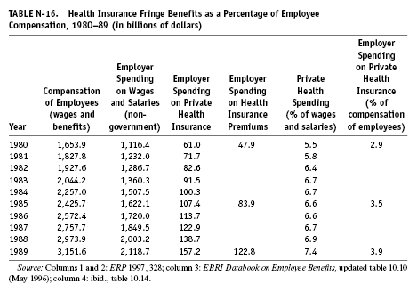
49. In support of the first set of numbers as the more accurate, the Council of Economic Advisers argues, “The [larger] estimates are obtained by adding up all the future repayments. . . . Such an estimate would be akin to claiming that a 10-percent 30-year, $100,000 home mortgage costs $315,925, which in fact is the undiscounted sum of the repayments required by that mortgage” (ERP 1991, 173). The word “undiscounted” is key, here. Income you receive in the future is worth less than the same amount of money received today—that’s why lenders demand, and borrowers are willing to pay, interest. Repayments in the future cost less in today’s dollars than they will when they have to be paid because, in anticipation of having to make that payment, one could invest a smaller sum and watch it grow to the amount needing to be paid out.
50. ERP 1991, 174.
51. ERP 1992, 26.
52. The wide range of estimates is based both on the wide range of possible impacts on the rate of interest (anywhere from 0.5 percent to 2.5 percent) paid by the government on its outstanding debt as well as the time rate of discount used to collapse the cost into present value terms. See Shoven, Smart and Waldfogel, “Real Interest Rates,” 266.
53. ERP 1991, 177.
54. This argument has been facetiously taken to its logical conclusion with the suggestion that the way to guarantee safe driving is to mandate that every steering wheel come equipped with a permanent harpoon aimed at the chest of the driver to guarantee that the driver will not collide with anything!
55. 1993 Green Book, 1525.
56. That’s real income, calculated in 1993 dollars. See Bureau of the Census, Current Population Reports, Series P 60, table H-1.
57. 1993 Green Book, 1530–31. For median income, see U.S. Bureau of the Census, table H-1.
58. 1993 Green Book, 1530–31.
59. 1993 Green Book, 1531. Interest, dividend, and rental income for the top 1 percent went from 24.6 percent of their total income to 21.8 percent in 1985, not so much because their received less interest, dividend, and rental income but because their ability to receive income in capital gains increased so dramatically.
60. Edward N. Wolff, “The Rich Get Increasingly Richer: Latest Data on Household Wealth during the 1980s,” Briefing Paper, Economic Policy Institute, 1992, 1.
61. Ibid.
62. Wolff calculates that between 1922 and 1989 (with twenty separate observations), three-fifths of wealth inequality can be attributed to income inequality and two-fifths to relative increases in stock prices to home prices (ibid., 12–13).
63. With such ownership concentrated heavily in the top 5 percent of the population. For the years 1980, 1985, and 1990 the income from capital for the top 5 percent and 1 percent of the population is detailed in table N-17.
64. Lawrence Mishel and Jared Bernstein, The State of Working America, 1992–93 (Armonk, NY: M. E. Sharpe, 1993), 140.
65. Ibid., 146.
66. 1993 Green Book, 1326.
67. Paul Krugman, “The Right, the Rich, and the Facts,” American Prospect 11 (fall 1992): 23–24. Note that the base year is 1977, not 1979, because the data set he used was a Congressional Budget Office study that did not collect information for 1979.
68. Ibid., 25.
69. Kevin Phillips, The Politics of Rich and Poor (New York: Random House, 1990).
70. Lindsey, The Growth Experiment, 82.
71. In 1990, both ratios began to fall, dominated by the decline in nominal interest rates that actually reduced total personal interest income in absolute terms between that year and 1993 (ERP 1997, 330).
72. See Bartley, The Seven Fat Years, 272–73.
73. Ibid., 278.
74. Alan Reynolds, “Upstarts and Downstarts,” National Review, August 31, 1992, 26.
75. Isabel V. Sawhill and Mark Condon, “Is U.S. Income Inequality Really Growing? Sorting Out the Fairness Question,” Policy Bites (Urban Institute), June 1992, 3–4. Tables N-18 and N-19 include the information referred to in their article.
76. Ibid., 4.
77. This battle still raged three years later. See, for example, “Dick Armey’s Research” letters from U.S. Representative Dick Armey (R.-TX) and a response by Michael Lind, New York Times Book Review, August 20, 1995, 27.
78. “The lower and upper boundaries are $18,500 and $55,000, respectively, in 1987 dollars and are applied to all years using the CPI-UXI price index” (Timothy Smeeding, Greg Duncan, and Willard Rodgers, “W[h]ither the Middle Class?” Policy Studies Paper No. 1, Metropolitan Studies Program, Income Security Policy Series, Maxwell School of Citizenship and Public Affairs, Syracuse University, February 1992, 5). The specifics of the index used need not concern us here. The important point is that once they have established an absolute standard of what constitutes the “middle class” the authors adjust that standard to take account of inflation for all the other years in the survey. This permits them to see if people who were in the absolutely defined middle class in 1967 stayed there over the next twenty-one years. Note that it is essential to have an absolute standard because if we merely identified the same ratio (between the lowest 20 percent and the top 10 percent) we would have the same number of households (70 percent of them) each year! Smeeding, Duncan, and Rodgers use another measure of the middle class that adjusts for family size. In this case, the middle class consists of families with incomes from two times to six times the family’s “poverty threshold,” which varies according to family size (in 1990 it was thirteen thousand dollars for a family of four). Their results show similar patterns for this measure and the original one. (I am indebted to Professor Smeeding for sending me this paper.)


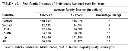
79. Smeeding, Duncan, and Rodgers, in “W(h)ither the Middle Class?” created table N-20, which they title “Percent of Adults Making Key Income Transitions.” The high-income transitions involve either a middle-income individual moving above the high-group threshold of income, or someone from that group “falling out” into the middle class. The low-income transitions involve either a middle-income person falling below the middle-class threshold or a person from that low-income group “climbing out” into the middle class. One should not be misled by the high percentages of high-income people “falling out” compared to the seemingly low percentage of middle-income people “climbing out” because, remember, the middle-income group represents close to 70 percent of the population, while the high-income group to begin with represents only 10 percent of the population, while the lower-income group is only 20 percent. In absolute numbers 6.7 percent of 70 percent of the population is much higher than 29.1 percent of 10 percent of the population. (If there were one thousand people in the population, 6.7 percent of 70 percent would be about forty-seven people, while 29.1 percent of 10 percent would be twenty-nine people!) Instead, the most important numbers above are the differences between the probabilities of social mobility before 1980 and after 1980.