1
Electromobility and the Environment

“My first customer was a lunatic. My second had a death wish.” Karl Friedrich Benz (1844–1929) is generally credited with pioneering the modern vehicle.

“Practically no one had the remotest notion of the future of the internal‐combustion engine, while we were just on the edge of the great electrical development. As with every comparatively new idea, electricity was expected to do much more than we even now have any indication that it can do. I did not see the use of experimenting with electricity for my purposes. A road car could not run on a trolley even if trolley wires had been less expensive; no storage battery was in sight of a weight that was practical … That is not to say that I held or now hold electricity cheaply; we have not yet begun to use electricity. But it has its place, and the internal‐combustion engine has its place. Neither can substitute for the other – which is exceedingly fortunate.” Henry Ford in 1923, reflecting on 1899.

“Any customer can have a car painted any color that he wants so long as it is black.” Henry Ford (1863–1947) was influenced by slaughterhouse practices when he developed his assembly line for the mass production of the automobile.

“The world hates change, yet it is the only thing that has brought progress.” Charles Kettering (1876–1958) invented the electric starter and effectively killed the electric car of that era.

“The spread of civilization may be likened to a fire: first, a feeble spark, next a flickering flame, then a mighty blaze, ever increasing in speed and power.” Nikola Tesla (1856–1943).

“Dum spiro, spero.” (Latin for “As long as I breathe, I hope.”) Marcus Cicero (106–43 BC). A noble aspiration from ancient times … but what if we can’t breathe the air?

“It was during that period that I made public my findings on the nature of the eye‐irritating, plant‐damaging smog. I attributed it to the petrochemical oxidation of organic materials originating with the petroleum industry and automobiles.” Aries Jan Haagen‐Smit (1900–1977), a pioneer of air‐quality control, reflecting in 1970 on his pioneering work from 1952 to explain the Los Angeles smog.

“Tesla’s mission is to accelerate the world’s transition to sustainable energy.” The 2016 mission statement of Tesla, Inc.

In this chapter, the reader is introduced to the factors motivating the development of the electric powertrain. The chapter begins with a brief history of the automobile from an electric vehicle perspective, the various energy sources, and the resulting emissions. Standardized vehicle drive cycles are discussed as drive cycles are used to provide a uniform testing approach to measure the emissions and the fuel economy of a vehicle, both of which are related to the efficiency of the energy conversion from the stored energy to kinetic energy. Government regulations and the marketplace have resulted in strong global trends to reduce these potentially harmful emissions and to increase the fuel economy. These factors of reduced emissions and improved efficiency combine with a greater consumer market appreciation for green technology to motivate the development of the electric powertrain. The competing automotive powertrains are briefly reviewed and discussed in terms of efficiency. The chapter concludes with a brief look at heavy‐duty commercial vehicles and other modes of transport.

1.1 A Brief History of the Electric Powertrain

There are three evolutionary eras of electric cars, and we shall now discuss the bigger historical picture.

1.1.1 Part I – The Birth of the Electric Car

The first self‐propelled vehicles were powered by steam. Steam vehicles were fueled by coal and wood and took a relatively long time to generate the steam to power the pistons by heating the furnace of an external combustion engine. The modern vehicle, first developed by Karl Benz in the 1880s, is based on the internal‐combustion (IC) engine. The early vehicles were unreliable, noisy, polluting, and difficult to start. Meanwhile, modern electrical technologies were being invented as Nikola Tesla, partnering with George Westinghouse, and Thomas Edison battled to invent and establish supremacy for their respective alternating‐current (ac) and direct‐current (dc) power systems. Battery electric vehicles (BEVs), energized by lead‐acid batteries and using a dc power system, competed with IC engine vehicles in the 1890s. Electric vehicles (EVs) did not have the starting problems of the IC engine and had no tailpipe emissions. The low range of the BEVs was not necessarily a problem at the time as the road system was not developed, and so comfortable roads were not available for long driving. In 1900, the sales of gasoline vehicles and EVs in the United States were comparable in quantity, but EV sales were to collapse over the next decade [1–4]. Interestingly, EV sales were poor in the Europe of this period as the French and German auto manufacturers, such as Renault, Peugeot, Daimler, and Benz, were leading the world in the development of the IC engine.

The dominance of the IC engine was to be established with two major developments. First, Henry Ford mass‐produced the Model T and drove down the sales price of the gasoline vehicle to significantly below that of both his competitors and of the EVs [5]. However, the gasoline vehicle still needed a manual crank in order to start the engine.

The second major development was the elimination of the manual crank by Charles Kettering’s invention of the electric ignition and start. These electric technologies were introduced by Cadillac in 1912 and, ironically, effectively consigned the BEV to history. As the electrically started gasoline cars proliferated, so did road systems. The mobility delivered by the car fostered the development of modern society as it stimulated individualized transportation and suburbanization. California became the poster child for these trends, which have spread globally. Given their low range and high costs, BEVs could no longer compete and the market died, expect for niche applications such as delivery trucks.

1.1.2 Part II – The Resurgent Electric Powertrain

The diesel engine was introduced for vehicles in 1922, 32 years after it was invented by Rudolf Diesel in 1890 as a more efficient compression‐ignition (CI) IC engine compared to the spark‐ignition (SI) IC engine fueled by gasoline. The first commercial diesel engines were actually developed by a spin‐off company of the US brewer Anheuser Busch. The high‐torque‐at‐low‐speed characteristic has made the diesel engine the engine of choice for medium and heavy‐duty vehicles worldwide. In recent times, the diesel engine became a choice for light vehicles, especially in Europe, due to its reduced carbon emissions compared to gasoline.

Of course, burning fossil fuels in the engine does not come without an environmental cost. A Dutch scientist, Aries Jan Haagen‐Smit, had moved to California and was perplexed by the pollution and smog in rapidly urbanizing Southern California. Smog is a portmanteau word combining smoke and fog to describe the hazy air pollution common in urban areas. London‐type smog is a term commonly used to describe the smog due to coal, while Los Angeles–type smog is used to describe the smog due to vehicle emissions. Haagen‐Smit demonstrated that California smog is the product of a photochemical reaction between IC engine emissions and sunlight to create ozone [6,7]. He is now known as the father of air pollution control and mitigation. The geography of Southern California features valleys, which tend to trap the pollutants for much of the year until the winds from the desert blow through the valleys in the fall. Similar geographic issues worsen the smog situations in other cities, such as Beijing – where the Gobi winds bring dust from the desert to combine with the city’s smog.

In the late 1980s, General Motors (GM) decided to develop an all‐electric car. The motivations were many. For example, urban pollution in American cities, especially Los Angeles, was severe. An additional significant motivating factor was the success of the solar‐powered Sunraycer electric car in the Solar Challenge, a 3000 km race across Australia in 1987. The Sunraycer was engineered by AeroVironment, General Motors‚ and Hughes Aircraft, who pushed the boundaries to develop the lightweight, low‐drag, solar‐powered electric car.

The initial GM prototype BEV, known as the Impact, was developed in Southern California, and GM committed to mass‐producing the car. The production vehicle, which was to become known as the GM EV1, was developed and produced at GM facilities in Michigan and Southern California, and made its debut in 1996. The vehicle was revolutionary as it featured many of the technologies which we regard as commonplace today. The improved traction motor was a high‐power ac induction motor based on the inventions of Nikola Tesla. The car body was built of aluminum in order to reduce vehicle weight. The vehicle aerodynamics were lower than any production vehicle of the day. The vehicle featured advanced silicon technology to control all the electronics in the vehicle and the new IGBT silicon switch to ensure efficient and fast control of the motor. This vehicle introduced electric steering, braking, and cabin heating and cooling. The EV1 featured extensive diagnostics, a feature that is now commonly employed in most vehicles to improve fuel economy and handling. Heavy‐duty vehicle prototypes for transit and school buses were also electrified and deployed in public by GM at this time. It is worth noting that electric powertrains have been commonly deployed by the railroad industry for many decades due to the inherent advantages of fuel economy and performance.

However, the GM EV1 went to market powered by lead‐acid batteries, a technology which had limited progress over the previous century. The second‐generation GM EV1 featured a nickel‐metal hydride (NiMH) battery which almost doubled the range of the first‐generation vehicle. However, a number of realities were to doom this particular effort – the inadequacy of battery technology, a collapse in the price of gasoline, a lack of consumer demand for energy‐efficient and green technologies, a lack of government support, and the advent of the hybrid electric car.

In the early 1990s, Toyota Motor Company was looking ahead at the challenges of the new century and also concluded that transportation had to become more efficient, more electric, and less polluting. Toyota first marketed the Toyota Prius in 1997 in Japan. The vehicle featured an extremely efficient gasoline engine based on the Atkinson cycle. While the efficient Atkinson‐cycle engine is not suitable as the engine in a conventional gasoline vehicle, Toyota overcame the engine limitations by hybridizing the powertrain to create a highly fuel‐efficient vehicle. The Toyota Prius featured a NiMH battery pack, the efficient IGBT silicon switch, and an ac motor featuring permanent magnets. The interior permanent‐magnet (IPM) motor features advanced rare‐earth permanent magnets to make the machine more efficient and power dense than its cousin, the induction motor. The Toyota Prius also eliminated the conventional transmission and developed the continuously variable transmission, commonly termed CVT. Toyota realized early on that the hybrid technology enabled a decoupling of the traffic condition from the engine use, such that the overall fuel economy could be maximized. The vehicle introduced technologies such as electric stop‐start and idle control, which have become common.

The gasoline‐sipping Toyota Prius and its siblings went on to become the mass‐market leaders for energy‐efficient and green technologies, and effectively ended the brief BEV flurry of the 1990s, while opening the world’s eyes to the value of the electric powertrain.

1.1.3 Part III – Success at Last for the Electric Powertrain

The basic limitation for electric cars in the industrial age has been the battery. Significant battery development efforts in the 1970s focused on the lithium battery. John Goodenough was credited with developing the first workable lithium‐ion (Li‐ion) cell in 1979. This technology was to be commercialized by Sony Corporation in 1991, and Li‐ion technology went on to become the battery of choice for mobile phones and laptop computers due to its high voltage and high energy density. The energy density of the Li‐ion cell could be three to five times higher than that for a lead‐acid cell, albeit at a higher price.

Pioneers of the GM Impact, Alan Cocconi and Wally Rippel, formed a company known as AC Propulsion and continued to work in the EV field with a focus on drive systems and chargers. AC Propulsion developed a prototype BEV, known as the tzero, shown in Figure 1.1, in the early 2000s. The unique attribute of these prototype vehicles was that they featured a very high number of computer laptop Li‐ion cells for the main storage battery. This development produced a very workable EV range whilst demonstrating both high efficiency and high performance.

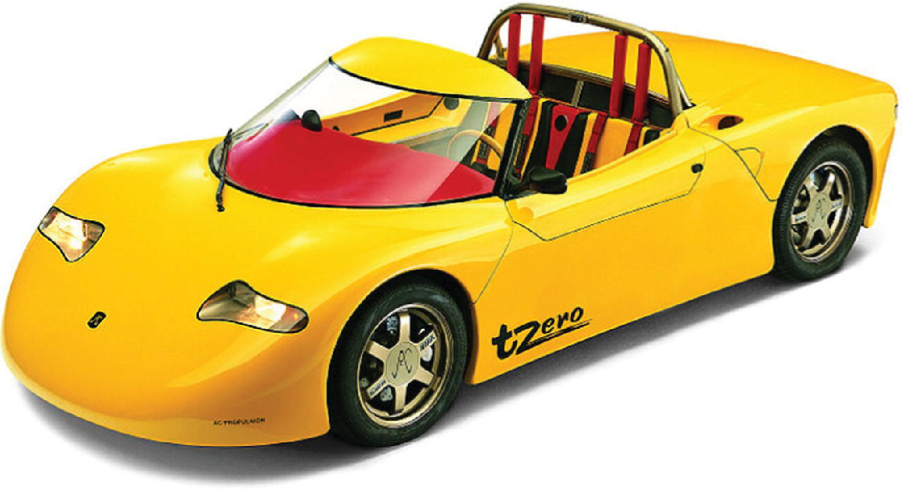
Figure 1.1 AC Propulsion tzero.

(Courtesy of AC Propulsion.)

These prototypes were to be test‐driven by Silicon Valley entrepreneurs, who urged commercialization of the technology. Tesla Motors was founded in Silicon Valley, and the first vehicle from Tesla was the Tesla Roadster in 2007. The Tesla Roadster was the first mass‐market EV featuring Li‐ion cells. It had a very high number of cells, 6,831 Panasonic cells in total.

Tesla built on the Roadster success with the subsequent introduction of the Tesla Model S luxury sedan in 2012, the Tesla Model X in 2015, and the Model 3 in 2017. The company, led by CEO Elon Musk, has very successfully competed in the automotive marketplace, and has attracted buyers globally to EVs. Long‐range batteries, high performance, autonomous driving, a more digital driver interface, direct sales, and photovoltaic solar power have all played a part in the Tesla vision for the vehicle [8].

The Nissan Leaf was introduced in 2011 and Nissan became the largest volume seller of EVs. The Nissan Leaf had a much lower price than the Tesla, making the car financially attractive for the mass‐market consumer, albeit with a much lower range.

The Tesla and Nissan vehicles were launched in a different era in California from that of the GM EV1. Critical market support was now available from the government. Using a system of credits, the EV manufacturers would effectively receive financial transfers from the other automotive manufacturers in order to subsidize the business model while the market developed. As the price of batteries continued to drop, more battery EVs came onto the market. In 2016, GM introduced the midrange Chevy Bolt, shown in Figures 1.2 and 1.3, while Tesla introduced the Model 3 in 2017, both vehicles with approximately 200 miles of range.

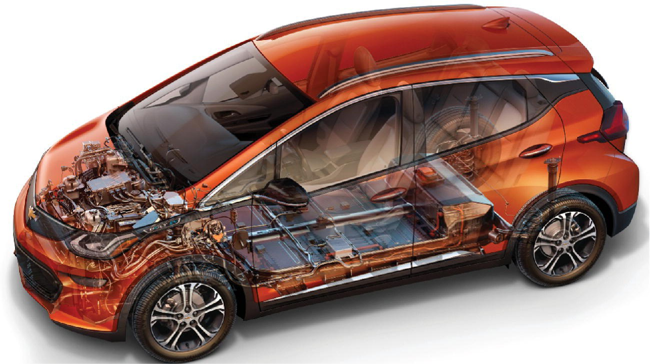
Figure 1.2 Chevy Bolt.

(Courtesy of General Motors.)

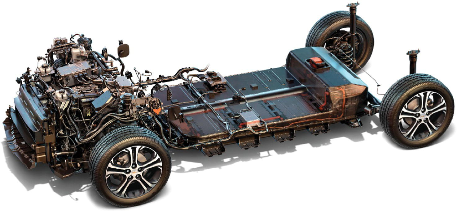
Figure 1.3 Battery and propulsion system of a stripped‐down Chevy Bolt.

(Courtesy of General Motors.)

Hybrid electric vehicles (HEVs) continue to dominate the EV market with multiple products from Toyota, Ford, Honda, Hyundai, BMW, Volkswagen, and others. A number of manufacturers are following General Motors’ Chevy Volt, a variant on a plug‐in hybrid electric vehicle (PHEV). The PHEV has a large enough Li‐ion battery to satisfy most drivers’ daily commutes, but it can run an on‐board gasoline engine efficiently to recharge the battery and provide propulsion power efficiently when needed.

Fuel cell vehicles with electric powertrains have also been introduced. Fuel cells have been around for a long time. For example, fuel cells have been used on spacecraft for decades. The automotive fuel cell converts stored hydrogen and oxygen from the air into electricity. The hydrogen must be highly compressed to obtain adequate storage on the vehicle. Advances in technology have reduced the size and cost of the fuel cell and the required balance of plant (a term used to describe the additional equipment required to generate the power). The attraction of the fuel cell electric vehicle (FCEV) is that it combines the electric powertrain with energy‐dense hydrogen and only emits water at the point of use. Thus, like the battery EV, the FCEV is zero emissions at the point of use. The fuel cell is an attractive option for vehicles as it can increase energy storage compared to the battery. Key challenges for the technology are the generation of hydrogen using low‐carbon methods and the development of a distribution and refueling system. Hyundai introduced the Tucson FCEV for lease in California in 2014. Toyota brought the Toyota Mirai FCEV to the market in 2015. Honda introduced the Clarity for limited lease in 2017 (following an earlier version released in 2008).

A major scandal erupted in the car industry in 2015 when it was established that Volkswagen had in effect been cheating in the Environmental Protection Agency (EPA) emissions testing [9]. During an emissions test, the Volkswagen car software would detect that the car was being tested and cause the vehicle to reduce various emissions in order to meet the EPA limits. Once the vehicle software decided that the vehicle was no longer being tested, the emission levels would increase.

Thus, one of the best diesel engine manufacturers in the world had struggled to meet the emission standards, and had done so by manipulating and circumventing the engine controller so as to meet the standards at the specified points, while exceeding the standards during ordinary driving. This case resulted in a multibillion dollar settlement with the US federal government and the state of California to fund the commercialization of zero‐emission vehicles, with significant investment in batteries and fuel cells.

In conclusion, the electric car has been well and truly revived in the twenty‐first century. There are many variations available ranging from battery electric to hybrid electric to fuel cell electric – hence the content of this book.

Finally, it must be noted that the world changed in the decades following the introduction of the GM EV1 in 1996. Significant consumer interest and a resulting market developed for green technologies. Local, state, and federal governments, the public, and industry awoke to the need to foster, and in some cases to subsidize, greener technologies. The motivations were many: minimize pollution to have tolerable air quality; reduce global warming to minimize climate change; develop local or greener energy sources to reduce energy dependence on more volatile parts of the world; and develop related businesses and industries.

History has burdened many of the oil‐producing countries with despotic regimes, wars, volatility‚ and instability. Many of the energy diversification and efficiency initiatives have been launched as a result of national security considerations due to supply‐chain volatility caused by war: the First Gulf War in 1991, the Second Gulf War in 2003, and so on. Together with the changing perceptions on pollution and climate change, these are all significant motivating factors to improve energy efficiency.

Wind and photovoltaic energy sources are commonly used in many countries around the globe. Efficiencies have improved due to regulations and consumer expectations. Compressed natural gas has become the fossil fuel of choice for electricity generation. The fracking of shale gas and oil has caused an energy revolution in the United States, and a shift away from “dirtier” fuels, such as coal. China has heavily industrialized using coal and now has very severe pollution problems. Nuclear power is once more viewed as problematic after a tsunami hit the Fukushima power plant in 2011 – with Germany deciding to abandon nuclear power as a result. There is increased usage of biofuels in transportation – based on sugarcane in Brazil and corn in the United States. Diesel fuel is viewed as problematic due to the significant NO_x emissions and the high cost per vehicle of treating the NO_x and particulate matter emissions.

Of course, there are many contradictions as countries adopt energy policies. Nuclear power can be perceived negatively due to associated risk factors but does result in low carbon emissions. The use of land for biofuels impacts food output and can raise food prices. Renewable sources can be intermittent and require problematic energy storage. There are many difficult choices, and we are limited by the laws of physics. The first law of thermodynamics is the law of conservation of energy. This law states that energy cannot be created or destroyed, but only changed from one form into another or transferred from one object to another.

Thus, much has changed since 1996 and will continue to change, as countries around the world adjust their energy sources and usage based on economic, environmental‚ and security factors … and the associated politics.

We next investigate some of the characteristics of these energy fuels.

1.2 Energy Sources for Propulsion and Emissions

In this section, we briefly consider the energy sources mentioned above. Characteristics of various fuels are shown in Table 1.1. The first four fuels are all fossil fuels. Gasoline is the most common ground‐transportation fuel, followed by diesel. Some related characteristics of gasoline, diesel, and compressed natural gas (CNG) are shown in Table 1.1. The main reference for the specific energy and density is the Bosch Automotive Handbook [10]. Coal is also included for reference and has many varieties, of which anthracite is one. There can be minor variations in the actual energy content of a fuel as the fuel is often a blend of slightly different varieties of fuel – and likely also including some biofuel, such as ethanol, in the mix. A formula is presented for a representative compound in the mixture.

Table 1.1 Energy and carbon content of various fuels.

Fuel	Representative formula	Specific energy		Density (kg/L)	Energy density (kWh/L)	CO2 emissions
		(kWh/kg)	(kJ/g)			(kgCO2/kg fuel)	(gCO2 /kWh)
Gasoline	C8H18 (iso‐octane)	11.1–11.6	40.1–41.9 [10]	0.72–0.775 [10]	8.0–9.0	3.09	266
Diesel	C12H23	11.9–12.0	42.9–43.1 [10]	0.82–0.845 [10]	9.8–10.1	3.16	268
Gas	C H4 (methane)	13.9	50 [10]	0.2	2.8	2.75	198
	Natural (mostly CH4)	11.2–13.0	40.2–46.7 [10]
Coal	C240H90O4NS (anthracite)	8	28.8	0.85	6.8	2.8	350
Hydrogen	H2	33.3	120 [10]	0.42 (at 700 bar)	14	0	0
Li‐ion		0.15	0.54	2.5	0.375	0	0

Gasoline and diesel have similar energy content per unit weight. Since diesel is a denser fluid than gasoline, it has a higher energy content by volume compared to gasoline. This higher energy content per unit volume, for example, per gallon, accounts for a significant portion of the fuel economy advantage that diesel has over gasoline. The combustion process is additionally more efficient for diesel than for gasoline.

In general, CNG has higher energy densities by mass compared to the liquid fuels, but has significantly lower energy density when measured by volume.

Hydrogen is the fuel of choice for fuel cell vehicles, and its characteristics are included here for comparison. Hydrogen has to be highly compressed. The 2016 Toyota Mirai uses 700 bar or 70.7 MPa pressure for the 5 kg of hydrogen on board. Significant additional vehicle volume is required for the storage components and required ancillaries.

Some approximate numbers are included for the Li‐ion battery pack. The specific energy and the energy density of the Li‐ion battery pack are approximately 76 times and 23 times lower than gasoline, respectively. Thus, battery packs have to be relatively large and heavy in order to store sufficient energy for EVs to compete with IC engine vehicles.

Note that the carbon content is calculated based on the formulae presented in column 2 of the table and by using the analysis presented in the next section. The energy content is based on approximate figures for the lower heating value (LHV) which is commonly referenced for the energy content of a fuel.

1.2.1 Carbon Emissions from Fuels

The IC engine works on the principle that the fuel injected into the cylinder can be combined with air and ignited by a spark or pressure. The resulting expansion of the gases due to the heat of the combustion within the cylinder results in a movement of the pistons which is converted into a motive force for the vehicle. The spontaneous thermochemical reaction within the IC engine cylinder has the following formula:

(1.1)

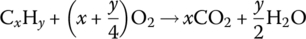
where the inputs to the reaction are C_xH_y, the generic chemical formula for the fossil fuel, as presented in Table 1.1, and O₂, the oxygen in the injected air [11]. The outputs from the reaction are heat, carbon dioxide (CO₂), and water (H₂O). The indices x and y are governed by the chemical composition of the fuel. Of course, it is air rather than pure oxygen which is input to the engine. As discussed in the next section, the 78% nitrogen content of the air can be a major culprit for emissions.

The engine can operate with various fuel‐to‐air ratios, and the particular mix can affect the emissions and fuel economy. A low fuel‐to‐air ratio is termed lean, and a high fuel‐to‐air is termed rich. For example, a rich mix can have less molecular oxygen in the combustion reaction, resulting in increased output of carbon monoxide and soot.

The chemical formula for the combustion of iso‐octane, part of the gasoline mixture, is

(1.2)

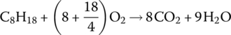
and for diesel combustion is

(1.3)

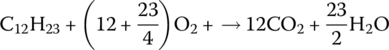
We can relate the carbon dioxide output from the combustion directly to the carbon content of the fuel and run some simple calculations to determine emissions.

1.2.1.1 Example: Carbon Dioxide Emissions from the Combustion of Gasoline

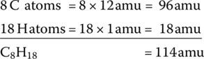
We can see that the x index of C₈H₁₈ results in eight CO₂ molecules for every C₈H₁₈ molecule. We next note that the molecular weights of the elements are different. The atomic mass unit of carbon, hydrogen, and oxygen are 12, 1, and 16, respectively. Thus, the atomic weight of C₈H₁₈ is 114 atomic mass units (amu), calculated as follows:

(1.4)

The atomic weight of the resulting CO₂ is

(1.5)

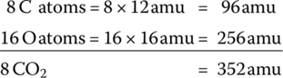
The relative difference of the molecular weights means that for every 1 kg of C₈H₁₆ fuel consumed in a thermochemical reaction, of carbon dioxide is produced. In other units, for every liter of gasoline consumed, about 2.39 kg of CO₂ is emitted. For every US gallon of gasoline consumed, about 9 kg (20 lb) of CO₂ are emitted.

1.2.2 Greenhouse Gases and Pollutants

There are a number of additional emissions from the combustion process – some causing ground‐level pollution and others contributing to the greenhouse effect. After‐treatment is a generic term used to describe the processing of the IC engine emissions on the vehicle, for example, by using a catalytic converter or particulate filter, in order to meet the vehicle emission requirements.

• Particulate matter (PM) is a complex mix of extremely small particles that are a product of the combustion cycle. The particles are too small to be filtered by the human throat and nose and can adversely affect the heart, lungs, and brain. They are also regarded as carcinogenic (cancer causing) in humans. A diesel engine can emit significantly more PM than the gasoline engine. The PM emissions can be mitigated by the after‐treatment, but at a significant financial cost. These particles are extremely small. In general, particles less than 10 µm in diameter (PM₁₀) are dangerous to inhale. PM_2.5 particles, which are less than 2.5 µm in diameter, can result from the combustion process and are a significant component of air pollution and a major contributor to cancers.
• Carbon monoxide (CO) is a colorless odorless gas that is a product of the combustion cycle. The gas can cause poisoning and even death in humans. Diesel engines produce lower levels of CO than spark‐ignition gasoline engines.
• A greenhouse gas (GHG) is any gas in the earth’s atmosphere which increases the trapping of infrared radiation, contributing to a greenhouse effect.
• Carbon dioxide (CO₂) is a greenhouse gas as it adds to the concentration of naturally occurring CO₂ in the atmosphere and contributes to the greenhouse effect. It is estimated that approximately 37 billion metric tons of CO₂ are released into the atmosphere every year due to the burning of fossil fuels by human activities [12].
• Nitrous oxide (N₂O) and methane (CH₄) are additional products of the combustion process which also contribute to the greenhouse effect. Methane, as a GHG, is often a product of the fossil fuel industry but can also result from livestock flatulence and other natural sources.
• Nitrogen oxide (NO), nitrogen dioxide (NO₂), and volatile organic compounds (VOCs) are emissions from the combustion process which result in ground‐level ozone and other pollutants. They are discussed in the next section.
• Total hydrocarbons (THCs) are hydrocarbon‐based emissions which contain unburnt hydrocarbons and VOCs. VOCs include alcohols, ketones, aldehydes, and more. THCs also contribute to greenhouse gases.

1.2.2.1 The Impact of NO_x

The air is composed of approximately 78% nitrogen, almost 21% oxygen, about 0.9% argon, about 0.04% CO_2, and minor quantities of other noble gases and water molecules. Although the nitrogen atoms are more tightly bonded together than the oxygen atoms, the elements can react under heat within the cylinders of the IC engine to make nitrogen oxide and nitrogen dioxide:

(1.6)

Compounds NO and NO₂ are commonly described as NO_x.

The nitrogen dioxide can then react in the sunlight to create atomic oxygen O and nitrogen oxide NO:

(1.7)

The atomic oxygen O can then react with molecular oxygen O₂ in the air to form ozone O₃:

(1.8)

Hydrocarbons are also produced by the combustion process. Included within the overall hydrocarbons are VOCs, which are essential for the buildup of ozone and smog at ground level. If VOCs were not present, then the ozone would react with the NO to create oxygen and remove the buildup of ozone. However, the VOC reacts with the hydroxide in the air and with the NO of Equation (1.7) to form NO₂.

The net effect of the overall reaction sequence involving the VOCs is that the ozone continues to build up in the atmosphere. The ground‐level ozone is inhaled by humans and other animals. The ozone reacts with the lining of the lung to cause respiratory illnesses such as asthma and lung inflammation. Note that atmospheric ozone is necessary in the upper atmosphere, known as the troposphere, in order to filter the sun’s harmful ultraviolet rays.

Another reaction of VOCs and NO_x results in peroxyacyl nitrates (also known as PANs), which can irritate the respiratory system and the eyes. PANs can damage vegetation and are a factor in skin cancer.

Diesel combustion engines are the major source of NO_x in urban environments. Cities such as London have experienced severe pollution in recent times due to the proliferation of diesel engines for light and heavy‐duty vehicles. It is projected that 23,500 people die each year in the United Kingdom due to the effects of NO_x [13]. Diesel has been seen by various governments as an important solution to carbon emissions, but the associated NO_x emissions have resulted in a significant degradation of the local air quality.

Many diesel vehicles use urea for emissions control. Urea CO(NH₂)₂ is a natural component of animal urine, and the compound is particularly useful in reducing NO_x. Industrially produced urea is stored in a tank on the vehicle and is injected into the exhaust system, where it is converted to ammonia. The ammonia reacts in the catalytic converter to reduce the NO_x. The overall reaction is as follows:

(1.9)

Undersized on‐board urea tanks contributed to the 2015 Volkswagen diesel emissions scandal [9].

A catalytic converter is an emissions‐control device installed on a vehicle to reduce the emissions of CO, THCs, and NO_x. Lead, also a pollutant, was eliminated from gasoline in order to facilitate the use of catalytic converters because lead coats the surface and disables the converter.

The catalytic converter has two main functions. First, it converts carbon monoxide and unburnt hydrocarbons to carbon dioxide and water:

(1.10)

Second, it converts the nitrogen oxides to nitrogen and oxygen:

(1.11)

Automotive emissions can impact on public health in many ways, and it is an area of active research (see the Further Reading section of this chapter). Hence, there is a serious movement toward the adoption of electric, hybrid, and fuel cell vehicles as the solution set to mitigate local pollution and carbon emissions.

1.3 The Advent of Regulations

The necessity for reduced vehicle emissions and associated emissions regulation by the government is evidenced here by California, which is only one part of a global problem. A brief outline of related events is presented in Table 1.2. This table is a modified version of the one presented on the web site of the Air Resources Board (ARB) of the California Environmental Protection Agency [14].

Table 1.2 Timeline of vehicle‐related developments in California.

1940	California’s population reached 7 million people with 2.8 million vehicles and 24 billion miles driven.
1943	First recognized episodes of smog occur in Los Angeles in the summer of 1943. Visibility is only three blocks, and people suffer from smarting eyes, respiratory discomfort, nausea, and vomiting. The phenomenon is termed a “gas attack” and blamed on a nearby butadiene plant. The situation does not improve when the plant is shut down.
1952	Over 4,000 deaths attributed to “Killer Fog” in London, England. This was London‐type smog.
	Jan Aries Haagen‐Smit discovered the nature and causes of photochemical smog. He determined that nitrogen oxides and hydrocarbons in the presence of ultraviolet radiation from the sun form smog (a key component of which is ozone). This was Los Angeles–type smog.
1960	California’s population reached 16 million people with 8 million vehicles and 71 billion miles driven.
1966	Auto tailpipe emission standards for HC and CO were adopted by the California Motor Vehicle Pollution Control Board, the first of their kind in the United States.
1968	Jan Aries Haagen‐Smit was appointed chairman of the recently formed Air Resources Board by Governor Ronald Reagan. (He was later fired by Reagan in 1973 over policy disagreements.)
	Federal Air Quality Act of 1967 was enacted. It allowed the State of California a waiver to set and enforce its own emissions standards for new vehicles.
1970	US EPA was created to protect all aspects of the environment.
1975	The first two‐way catalytic converters came into use as part of the ARB’s Motor Vehicle Emission Control Program. CAFE standards introduced by US Congress.
1980	California’s population reached 24 million people with 17 million vehicles and 155 billion miles driven.
1996	Big seven automakers commit to manufacture and sell zero‐emission vehicles. Debut of GM EV1.
1997	Toyota Prius debuts in Japan.
2000	California’s population grows to 34 million with 23.4 million vehicles and 280 billion miles driven.
	A long‐term children’s health study funded by the ARB revealed that exposure to high air pollution levels can slow down the lung function growth rate of children by up to 10%.
2007	Debut of Tesla Roadster.
2008	ARB adopts two critical regulations aimed at cleaning up harmful emissions from the estimated one million heavy‐duty diesel trucks. One requires the installation of diesel exhaust filters or engine replacement, and the other requires installation of fuel‐efficient tires and aerodynamic devices.
2010	California adopts the Renewable Energy Standard. One‐third of the electricity sold in the state in 2020 to come from clean, green sources of energy.
2011	ARB determines that 9,000 people die annually due to the amount of fine particle pollution in California’s air. Debut of Nissan Leaf.
2014	Hyundai fuel cell vehicle debuts in California.
2015	Volkswagen diesel emissions scandal becomes a big news story.

As the timeline in the table illustrates, expanding populations in developed countries embracing use of the automobile, and other technological advances, can generate significant pollution and greenhouse gases. The 280 billion miles driven in California in 2000 would have generated about 0.5 kg of CO₂ per mile or 140 billion kg of CO₂. However, this amounts to only a small fraction of the close to 37 billion metric tons of annual CO₂ emissions emitted globally by 2015 [12]. While smog was the original motivating factor, the public interest in controlling CO₂ emissions is significant as the emissions are directly related to fuel economy.

In 1975 the United States Congress introduced the Corporate Average Fuel Economy (CAFE) standards. These standards are resulting in a significant improvement in average fuel economy for cars and light trucks, with the projected fuel economy in 2025 being 54.5 mpg. The standard fuel economy was 18 mpg in 1978.

1.3.1 Regulatory Considerations and Emissions Trends

As discussed earlier, vehicles can significantly impact the global and local environments due to the emissions of greenhouse gases and associated urban smog and pollution. In addition, the use of gasoline and diesel as fuels raises considerations related to the security of the supply and the economics of such a critical commodity. Thus, there has been greater regulation of vehicle emissions and fuel economy in recent decades. Global historical and projected trends in CO₂ emissions and fuel consumption are shown in Figure 1.4, as compiled by the International Council on Clean Transportation (ICCT). The horizontal axis represents time, whereas the primary vertical axis represents the carbon emissions in gCO₂ per km normalized to the New European Drive Cycle (NEDC), a commonly referenced drive cycle standard. Globally, there has been a significant reduction in new‐vehicle emissions, and these trends are projected to continue to 2025 and beyond. For example, passenger car emissions in the United States are projected to decrease from 205 gCO₂ per km in 2002 to 98 gCO₂ per km in 2025. As fuel consumption is closely related to the carbon emissions, the same plots correlate to the fuel consumption in liters of fuel per 100 km plotted against the secondary vertical axis. Fuel consumption in the United States is projected to decrease from 8.7 L/100 km in 2002 to 4.1 L/100 km in 2025. Clearly, similar trends are happening globally.

Figure 1.4 Global trends in gCO₂/km (left axis) and L/100 km (right axis) normalized to NEDC.

(Courtesy of ICCT.)

1.3.2 Heavy‐Duty Vehicle Regulations

As with light‐duty vehicles, heavy‐duty vehicles are subject to greater emission controls. Light‐duty vehicles have a maximum gross vehicle weight of less than 3,855 kg (8,500 lb) in the United States, whereas heavy‐duty vehicles typically are up to 36,280 kg (80,000 lb).

European standards are widely referenced. Euro I was introduced for trucks and buses in 1993. The Euro VI standard was introduced for trucks and buses in 2014. As shown in Figure 1.5, the permitted emissions levels for NO_x and PM have been reduced significantly. This pattern of reduction can be credited to costly on‐board after‐treatment of diesel emissions. The emissions have been reduced from 8 g/kWh and 0.6 g/kWh in Euro I for NO_x and PM, respectively, to 0.4 g/kWh and 0.01 g/kWh in Euro VI.

Figure 1.5 Euro III to VI for heavy‐duty diesel engines.

Commercial vehicles such as freight trucks and passenger buses can be – and are being – hybridized for a number of commercial reasons, which do not necessarily apply to light‐duty vehicles:

• These vehicles often have defined drive cycles with defined routes, and locations with available trained user and service personnel.
• There can be significant maintenance and service costs, and so the vehicles can benefit from the lower failure rates and lower service costs associated with electrification.
• Municipal constraints on emissions, especially NO_x and PM, make it more difficult to drive non‐zero‐emission vehicles in urban areas.
• The heavy‐duty vehicles tend to have higher continuous power levels and lower relative peak power levels than the light‐duty vehicle.
• After‐treatment has been used to reduce the NO_x and PM emissions from diesel engines. However, after‐treatment is not cheap and can add several thousand dollars to the cost of a heavy‐duty diesel vehicle. While after‐treatment has been the main tool for mitigating the effects of NO_x and PM emissions, it provides no direct benefit to GHG or CO₂ reduction. The reductions in GHG and CO₂ are mostly due to power plant optimization by utilizing hybrid configurations, or the hydrogen fuel cell, and by downsizing the engines to run more efficiently.

All these factors are resulting in increased electrification of the heavy‐duty vehicle.

1.4 Drive Cycles

A drive cycle is a standardized drive profile which can be used to benchmark and compare fuel economy and emissions. Tests are conducted by operating vehicles using a professional driver driving on a flat treadmill‐type device called a dynamometer.

There are many types of standardized drive cycles in use around the world. The Worldwide Harmonized Light Vehicles Test Procedures (WLTP) has been developed for adoption in a number of countries. JC08 is a commonly referenced standard in Japan. Drive cycles created and managed by the EPA are commonly referenced in the United States.

This section focuses on the EPA drive cycles as they are widely referenced in the literature and media. The NEDC is commonly referenced in Europe. However, the NEDC is not as representative of real‐world driving considerations or as rigorous as the EPA tests, and it can significantly overpredict fuel economy and underestimate fuel consumption and emissions, as will be noted later.

1.4.1 EPA Drive Cycles

The standard US EPA fuel economy estimates are based on testing from five different drive cycles [15–18]. The vehicle exhaust emissions during a test are gathered in bags for analysis. There are four basic cycles used by the EPA, as shown in Table 1.3: FTP, HFET, US06, and SC03. The fifth test is a cold‐ambient FTP, termed FTP (cold).

Table 1.3 Drive cycle parameters.

Drive cycle	Distance (km)	Time (s)	Average speed (km/h)	Maximum speed (km/h)	HVAC
FTP	17.66	1874	33.76	90
FTP (cold)	17.66	1874	33.76	90	Heat
HFET	16.42	765	77.28	95
USO6	12.82	596	77.39	127
SCO3	5.73	596	34.48	88	AC
UDDS (LA4)	11.92	1369	31.34	90
NEDC	11.02	1180	33.6	120

The Federal Test Procedure FTP drive cycle is for city driving and is as shown in Figure 1.6(a). The FTP cycle is based on the earlier LA4 cycle, which is also known as the Urban Dynamometer Drive Schedule or UDDS, and was originally created based on Los Angeles driving. The initial 1400 s of the FTP cycle is the same as that of the full LA4 cycle. The first 450 s of the LA4 cycle is included after the full LA4 cycle to create the full FTP drive cycle. The Highway Fuel Economy Driving Schedule or HFET drive cycle, as shown in Figure 1.6(b), simulates highway driving. A higher‐acceleration, more aggressive cycle is based on the USO6 drive cycle, as shown in Figure 1.6(c). The use of air‐conditioning in city driving is introduced in the SCO3 drive cycle, as shown in Figure 1.6(d), and the testing is conducted at a hot ambient of 95 °F. The tests factor in varying temperature conditions and the effects of cold and hot starts. The contributions of the various tests are based on driving profiles of the typical American driver, as compiled by the EPA, and the results of the tests are compiled and adjusted in order to generate a realistic estimate of fuel economy, consumption, emissions, and range.

Figure 1.6 EPA drive cycles.

For comparison purposes, all the drive cycles shown in Figure 1.6 are plotted with 140 km/h on the speed axis. Some key parameters for the various tests are noted in Figure 1.6 and Table 1.3. Clearly, HFET and US06 are the highest speed tests. Note that the parameters for the LA4 and NEDC drive cycles are also included in Table 1.3.

The five‐cycle tests are based on the IC engine. The tests measure various emissions and fuel economy for given conditions. There can be significant variations in emissions and fuel economy depending on whether a vehicle is starting cold or is already warmed up, or if the vehicle requires heating, ventilation, or air‐conditioning (HVAC), as shown in the final column of Table 1.3. The various tests capture the significant conditions.

The testing is conducted by the manufacturer or the EPA, and the data are summarized and published annually by the EPA [16].

Table 1.4 shows EPA test data on the 2017 Toyota Prius Eco. The commonly referenced carbon dioxide emissions (CO₂) are shown in the second column. The emissions in grams per mile (g/mile) related to the THCs, carbon monoxide (CO), the oxides of nitrogen (NO_x), PM, methane (CH₄), and nitrous oxide (N₂O) are shown in the next several columns of the table. The final column presents the fuel economy in miles per US gallon (mpg) for the drive cycle.

Table 1.4 EPA data on 2017 Toyota Prius Eco emissions and fuel economy.

Drive cycle	CO2 (g/mile)	THC (g/mile)	CO (g/mile)	NOx (g/mile)	PM (g/mile)	CH4 (g/mile)	N2O (g/mile)	Unadj. fuel economy (mpg)
FTP	105	0.0117	0.0644	0.0029		0.0019	0.0013	84.1
FTP (cold)	153	0.1906	1.0590	0.0229				56.6
HFET	115	0.0004	0.0156	0.0001		0.0003		76.9
USO6	176	0.0249	0.201	0.0052				50.1
SCO3	152	0.0406	0.2768	0.0036				58

From Figure 1.6, it can be seen that the FTP, FTP (cold), and SC03 have similar average and maximum speeds, as they are all for city driving. However, because the vehicle is using additional fuel for heat for FTP (cold) and for air‐conditioning for SC03, the emissions and fuel economy can vary relatively significantly. The fuel economy decreases by 33% from FTP at 84.1 mpg to 56.6 mpg for FTP (cold), and by 31% to 58 mpg for SC03. The aggressive driving pattern of US06 results in the lowest fuel economy of 50.1 mpg. The HFET cycle has a relatively high fuel economy of 76.9 mpg.

The results of the various tests are combined to generate overall fuel economy numbers for consumer education and vehicle labeling [19]. The fuel economies from the five tests are combined in order to generate fuel economy estimates based on real‐world considerations for city, highway, and combined. The fuel economy estimates for various vehicles are as shown later in Table 1.8. The estimates for the 2017 Toyota Prius Eco are 58 mpg for city, 53 mpg for highway, and 56 mpg combined.

While the Toyota Prius Eco is one of the most efficient gasoline‐fueled vehicles on the road, diesel engines are generally used for heavy‐duty vehicles, and are also very popular in Europe for light vehicles due to increased fuel economy. The data for the 2015 Mercedes‐Benz ML250 Bluetec 4MATIC diesel vehicle are shown in Table 1.5. Obviously, given the relative size and enhanced performance of the vehicle compared to the 2017 Toyota Prius Eco, the fuel economy is significantly lower for the ML250. The NO_x and PM columns are significant factors when assessing the diesel engine.

Table 1.5 EPA data on 2015 Mercedes‐Benz ML250 BlueTEC 4MATIC emissions and fuel economy.

Drive cycle	CO2 (g/mile)	THC (g/mile)	CO (g/mile)	NOx (g/mile)	PM (g/mile)	CH4 (g/mile)	N2O (g/mile)	Unadj. fuel economy (mpg)
FTP	345	0.0185	0.09	0.025	0.0015	0.0130	0.01	29.5
FTP (cold)	471	0.0136	0.2069	0.4839	0.0043			21.6
HFET	233	0.0002	0.0049	0.0001	0.0011	0.0011	0.01	43.7
USO6	388	0	0.0053	0.1276	0.0004			26.2
SCO3	446	0.0017	0.0033	0.0950	0.0026			22.8

It is worth comparing the emissions for gasoline and diesel options from the same manufacturer, a HEV from Toyota, and the Tesla Model X 90D BEV, as shown in Table 1.6. The gasoline 2015 Mercedes‐Benz ML350 4MATIC is compared with its diesel sibling just discussed above for the city (FTP) and highway (HFET) drive cycles. As the diesel engine is larger and heavier than the gasoline engine, the diesel vehicle mass is heavier, as shown in column 4 of the table. The CO₂, THC, and CO emissions are higher for the gasoline engine compared to the diesel engine for city FTP driving, while NO_x and CH₄ drop comparatively for the diesel engine in highway HFET driving. There are significant emissions of PM and NO_x from the diesel vehicle during the city driving.

Table 1.6 Comparison of conventional gasoline, diesel, hybrid‐electric and battery‐electric vehicles.

Drive cycle	Model	Fuel	Power (kW)	Mass (kg)	CO2 (g/mile)	THC (g/mile)	CO (g/mile)	NOx (g/mile)	PM (g/mile)	CH4 (g/mile)	N2O (g/mile)	Unadj. fuel economy (mpge)
FTP	ML250	Diesel	150	2495	345	0.0185	0.09	0.0250	0.0015	0.0130	0.01	29.5
	ML350	Gasoline	225	2381	404	0.0365	0.7445	0.0054		0.0095		21.9
	RX450h	Gas. HEV	183	2268	215	0.0072	0.0756	0.0048				41.2
	Model X 90D	BEV	310	2495								124.2
HFET	ML250	Diesel	150	2495	233	0.0002	0.0049	0.0001	0.0011	0.00112	0.01	43.7
	ML350	Gasoline	225	2381	285	0.019	0.2948	0.0028		0.00728		31.1
	RX450h	Gas. HEV	183	2268	229	0.0003	0.0400	0.0017				38.7
	Model X 90D	BEV	310	2495								135.8

When the Lexus RX 450 h HEV from Toyota is considered, then the emissions decrease significantly for the HEV compared to the non‐hybrid vehicles, and the fuel economy increases significantly.

The advantage of hybridization now becomes clear. The HEV can achieve an efficiency for highway driving that is comparable with diesel, but the HEV can deliver similar fuel economy for stop‐and‐go city driving, unlike the diesel vehicle. While the carbon emissions are comparable for the HEV and diesel on the highway, the diesel fuel economy of 43.7 mpg is higher than that of the HEV at 38.7 mpg only because diesel fuel contains more energy per unit of volume.

The final option in the table is the Tesla SUV BEV. The advantages of the BEV become clear in this comparison. The equivalent mpg is significantly higher for the BEV than for all the other options, and without tailpipe emissions, albeit at the expense of reduced range.

1.5 BEV Fuel Consumption, Range, and mpge

Similarly, BEVs are characterized for fuel economy and consumption – vehicle tailpipe emissions do not need to be considered as there are no emissions from the vehicle.

The fuel economy of a BEV is actually specified using mpg equivalent, or mpge. A US gallon of gasoline nominally contains 33.705 kWh of energy, and so this value is used to determine mpge. Thus, the 90 kWh Tesla Model X 90D contains the equivalent energy of 2.67 US gallons. The BEV powertrain is far more efficient than the IC engine powertrain, and so the mpge of the BEV can be quite high, although the stored energy is low.

There are a number of ways of calculating fuel consumption and emissions. Typically, the BEV fuel economy is calculated using a two‐cycle test, as defined by the EPA [18,20]. Basically, the vehicle performance is measured for city and highway driving. The combined fuel economy is based on 55% city driving and 45% highway driving.

As the testing is conducted on a dynamometer, the combined fuel consumption is adjusted by dividing by 0.7 in order to factor in a realistic adjustment for real‐world driving and the use of HVAC.

Thus, the adjusted combined fuel consumption (FC) is given by

(1.12)

where cityFC is the fuel consumption measured for the city drive cycle (FTP) and hwyFC is the fuel consumption measured for the highway (HFET) drive cycle.

The manufacturer data on fuel consumption, measured as electrical kWh/100 miles from the charging plug, is published by the EPA and is shown in column 2 of Table 1.7. For example, the 2015 Nissan Leaf consumes 18.65 kWh and 23.28 kWh from the electrical grid in order to complete 100 miles of the city and highway drive cycles, respectively. These numbers are converted to units of Wh/km in column 3. The adjusted combined fuel consumption is calculated as 29.62 kWh/100 miles or 184.1 Wh/km based on Equation (1.12).

Table 1.7 2015 Nissan Leaf test results.

	(kWh/100 mile)	(Wh/km)	mpge
City FC	18.65	115.8	180.7
Hwy FC	23.28	144.7	144.8
Combined FC	20.73	128.8	162.6
Adj. City FC	26.64	165.6	126.5
Adj. Hwy FC	33.26	206.7	101.3
Adj. Combined FC	29.62	184.1	113.8
Range @ BOL	153 km (95 miles)
Range @ EOL	123 km (76 miles)
Range @ Midpoint	138 km (86 miles)

We can go further and estimate the vehicle range. If a charging efficiency of 85% is assumed, then the energy consumption from the battery is 85% of 184.1 Wh/km, or 156.5 Wh/km. Dividing this fuel consumption into the battery capacity of 24 kWh at the battery beginning of life (BOL) provides a range estimate of 153 km (95 miles).

As the battery capacity can decay with a number of factors, we note that the range drops proportionately to 122 km (76 miles) if the battery end‐of‐life (EOL) capacity is 80% of the BOL capacity. The EPA rating is the midpoint at 90% of BOL for an estimated range of 138 km (86 miles). The actual EPA range for the 24 kWh Nissan Leaf is 137 km, which compares well to the 138 km just estimated. The minor error between the two values can be related to the storage capacity or the charging efficiency assumption.

The NEDC range for the same vehicle is 200 km. The NEDC number is an unadjusted number based on dynamometer testing only. Following on the example above, it is clear that a reduction of at least 30% is needed in order to take into account real‐world driving scenarios, and would produce a more useful range estimate for the consumer.

The mpge can be easily calculated using the FC values. The mpge is related to the fuel consumption by the following formula:

(1.13)

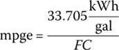
where FC is the fuel consumption in kWh/mile. The published EPA mpge values for adjusted city, highway, and combined driving are 126, 101, and 114 mpge, respectively, and these values are the same as those based on the calculations above, when rounded.

1.6 Carbon Emissions for Conventional and Electric Powertrains

It is useful to compare the overall emissions of a vehicle when considering the overall energy efficiency and environmental impact. In this section, we briefly review the carbon emissions related to the various powertrains. The EPA presents estimated carbon emissions for the various powertrains on its web site [19]. The EPA estimates consider the vehicle tailpipe emissions and the upstream emissions due to the production, transportation, and distribution of the various energy sources.

Note that these numbers are based on EPA data available in early 2017. At the time of publication the upstream emissions figures are not available for fuel cell vehicles, such as the Toyota Mirai. In general, it is expected that vehicle and grid emissions will continue to decrease as both vehicles and the grid become less polluting and more efficient.

EPA data on energy consumption and carbon emissions are presented in Table 1.8 for various midsize and large BEV, HEV, diesel, and gasoline vehicles. The 2017 Nissan Leaf consumes 30 kWh from the electrical grid per 100 miles driven, and this translates in a combined fuel economy of 112 mpge.

Table 1.8 Fuel economy, upstream carbon emissions, and range for various 2015–2017 vehicles (based on 2017 data).

Vehicle	Type	Size	Fuel economy			gCO2e Emissions total (tailpipe)	Range
			City	Highway	Combined
			(mpge)	(mpge)	(mpge)	(gCO2e/mile)	(miles)
2017 Nissan Leaf	BEV	Midsize	124	101	112	100 (Los Angeles)	107
						180 (United States)
						240 (Detroit)
2017 Hyundai Ioniq	BEV	Midsize	150	122	136	90 (Los Angeles)	124
						150 (United States)
						200 (Detroit)
2017 Chevy Volt	PHEV	Compact			106	140 (Los Angeles)	53 (electricity) 420 (total)
						200 (United States)
						250 (Detroit)
2017 Toyota Prius Eco	HEV	Midsize	58	53	56	190 (158)	633
2017 BMW 328d Auto	Diesel	Compact	31	43	36	346 (285)	540
2017 BMW 320i Auto	Gasoline	Compact	23	35	28	381 (323)	422
2017 Toyota Mirai	Hydrogen	Midsize	67	67	67	Not available	312
2017 Tesla Model X AWD 90D	BEV	SUV	90	94	92	130 (Los Angeles)	257
						220 (United States)
						300 (Detroit)
2017 Lexus RX 450 h AWD	HEV	SUV	31	28	30	356 (297)	516
2015 Mercedes‐Benz ML250 Bluetec 4MATIC	Diesel	SUV	22	29	25	499 (413)	615
2015 Mercedes‐Benz ML350 4MATIC	Gasoline	SUV	18	22	19	561 (456)	467
2015 Honda Civic	CNG	Compact	27	38	31	309 (218)	193
2015 Honda Civic	HEV	Compact	43	45	44	242 (202)	581
2015 Honda Civic HF	Gasoline	Compact	31	40	34	314 (259)	449

The EPA web site provides the option of estimating grid emissions on the basis of the local ZIP or postal code, as well as the national average. Let us compare two contrasting cities. The city of Los Angeles in California, with ZIP code 90013, has a relatively low‐emissions electrical grid. The city of Detroit in Michigan, with ZIP code 48201, has relatively high emissions due to the use of coal.

Thus, while the carbon emissions at the point of use for the 2017 30 kWh Nissan Leaf are zero, the upstream carbon emissions from the electric power stations can result in emissions ranging from 100 gCO₂/mile (62 gCO₂/km) in Los Angeles to 240 gCO₂/mile (149 gCO₂/km) for Detroit, with a national average of 180 gCO₂/mile (112 gCO₂/km).

The 2017 Hyundai Ioniq BEV has a 28 kWh battery pack and a longer range and higher efficiency than the 2017 Nissan Leaf. The EPA range for the vehicle is 124 miles, and the emissions are as low as 150 gCO₂/mile nationally in the United States.

The Chevy Volt PHEV can run 53 miles on battery only and 420 miles in total. The vehicle’s carbon emissions are estimated at 140 gCO₂/mile in Los Angeles and up to 250 gCO₂/mile in Detroit. The EPA assumes that the car is driven using the battery for 76.1% of the time and the balance using the gasoline engine.

The Toyota Prius Eco model has a combined fuel economy of 56 mpg with total carbon emissions, including upstream, of 190 gCO₂/mile, or 158 gCO₂/mile from the tailpipe. The BMW 320 series is presented for examples of the midsize diesel and gasoline vehicles. The total emissions are 346 and 381 gCO₂/mile for the diesel 328d and gasoline 320i vehicles, respectively.

EPA data on the 2016 Toyota Mirai fuel cell EV are included. The published fuel economy is 66 miles per kg of hydrogen, or 67 mpge, with a range of 312 miles.

Electric, hybrid, diesel, and gasoline SUV models are next considered. The all‐electric high‐performance Tesla Model X has a fraction of the upstream emissions compared to its competitors from Lexus and Mercedes‐Benz, with the conventional Mercedes vehicles having far higher emissions than the hybrid Lexus.

Finally, CNG is a competitive fuel for use in the spark‐ignition IC engine. As discussed earlier, CNG produces less gCO₂ than gasoline per kg of fuel. Even though CNG is less efficient than gasoline when combusted in the engine, a reduced value of the gCO₂/mile is expected overall. Honda Motor Company sold three versions of the Honda Civic in 2015: CNG, gasoline, and gasoline hybrid. A comparison of the vehicles illustrates the advantages and disadvantages of CNG. The tailpipe emissions of the CNG vehicle at 218 gCO₂/mile is an improvement on the conventional gasoline vehicle at 259 gCO₂/mile, but higher than the hybrid gasoline vehicle at 202 gCO₂/mile. The range of the CNG vehicle is less than half of the range of the other vehicles due to the larger storage required for the CNG. The upstream emissions for the CNG vehicle are disproportionately higher than those of the gasoline vehicles. Equivalent CO₂ or CO₂e is the concentration of CO₂ which would cause the equivalent effect with time as the emitted greenhouse gases, especially methane. Leakage of methane during production, transmission, and distribution of CNG has a significantly greater impact as a greenhouse gas over time than CO₂, resulting in increased gCO₂ equivalent emissions for CNG. Thus, the total emissions for the CNG vehicle at 309 gCO₂/mile are only a little lower than those of the gasoline vehicle at 314 gCO₂/mile, and significantly higher than those of the hybrid vehicles at 242 gCO₂/mile.

1.6.1 Well‐to‐Wheel and Cradle‐to‐Grave Emissions

Well to wheel is the term used to describe the overall energy flow from the oil or gas well when the fossil fuel comes out of the ground to the ultimate usage in the vehicle to spin the wheels. It is an area of active research and application. For example, Argonne National Laboratory in the United States has developed the widely referenced GREET (Greenhouse gases, Regulated Emissions, and Energy use in Transportation) model for use in this area [21–23]. The GREET model is used to estimate emissions in the EPA models.

There are significant energy and carbon costs incurred during the production of a vehicle. Reference [24] provides a comprehensive study into the equivalent carbon required for the cradle‐to‐grave emissions assessment of the conventional Ford Focus IC engine vehicles compared to the battery electric version of the Ford Focus. The BEV version incurred about 10.3 metric tons of CO₂e compared to about 7.5 metric tons of CO₂e for the Ford Focus IC engine vehicle. The emissions of CO₂e for the 24 kWh Li‐ion battery alone were 3.4 metric tons, or 140 kg per kWh. Reference Problem 1.3.

1.6.2 Emissions due to the Electrical Grid

All EVs have the advantage of zero carbon emissions from the vehicle itself. Clearly, there are emissions at some point in the energy conversion process if fossil fuels are used to generate the electricity for BEVs or compressed hydrogen for FCEVs. Coal is used as the base load in many electricity grids as it is abundant and cheap. The carbon emissions from coal are relatively high compared to the other fossil fuels. It also outputs significant amounts of sulfur dioxide (SO₂) in addition to the nitrogen oxides. Sulfur dioxide is a significant component of urban smog. Atmospheric sulfur dioxide can react with oxygen and then water to create sulfuric acid, the main component of harmful acid rain. Coal fuel has resulted in major problems for populous countries such as China, India, and the United States. Low‐sulfur coal can mitigate the problem and is available in abundance in various regions of the world.

Many electrical grids employ coal for the base load and gas as a more flexible and cleaner fuel. The balance of energy is typically provided by nuclear, hydroelectric, and renewable sources. It is useful to estimate the carbon emissions due to the production of electricity. Typical power plant efficiencies range from about 38% for coal to around 50% for gas [25].

1.6.2.1 Example: Determining Electrical Grid Emissions

Determine the carbon emissions from the electrical grid in gCO₂/kWh(electrical) if 35% of the electricity comes from coal and 40% comes from gas, with the balance being carbon‐free nuclear, hydroelectric, and renewables. Adjust your answer higher by 20% to allow for fuel production and distribution, and electricity transmission and distribution.

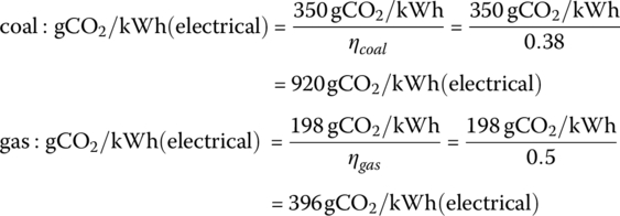
Representative power plant efficiency values are η_coal = 38% for coal and η_gas =50% for gas. Carbon emissions for coal and gas are presented in Table 1.1.

Solution:

The carbon emissions are 198 gCO₂/kWh for gas and 350 gCO₂/kWh for coal from Table 1.1. These emission values are based on the primary (or embedded) energy of the fuel. The carbon emissions for the energy output as electricity is lower due to the efficiencies of the power plants.

These emissions numbers must be divided by the power plant efficiencies in order to determine the emissions for each unit of output electrical energy:

The emissions are then prorated according to their grid usage:

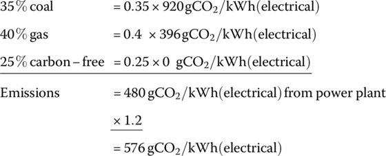
Thus, the overall emissions are 576 gCO₂/kWh(electrical) for this representative example.

1.7 An Overview of Conventional, Battery, Hybrid, and Fuel Cell Electric Systems

Seven vehicle architectures are considered in this section and over the next four chapters:

1. Conventional vehicles with IC engine:
   1. CI IC engine using diesel
   2. SI IC engine using gasoline or CNG
2. Battery electric
3. Hybrid electric:
   1. Series
   2. Parallel
   3. Series‐parallel
4. Fuel cell electric

Simplified vehicle configurations are discussed next. The vehicle and overall well‐to‐wheel efficiencies are briefly considered. While vehicle efficiencies obviously depend on driving patterns and other factors, representative figures are used in this section to illustrate the differences.

1.7.1 Conventional IC engine Vehicle

The IC engine is coupled via a clutch and gearing through the transmission to the drive axle. The elementary figure of Figure 1.7 simply represents the conventional powertrain. This basic architecture is the basis for the modern vehicle.

Figure 1.7 Conventional vehicle architecture and energy flow.

The percentage engine efficiency η_eng can range from very low values to the mid‐to‐high 30s for gasoline to the 40s for diesel. An overall tank‐to‐wheel vehicle efficiency η_T‐W of 20% is representative for a conventional diesel vehicle, with lower values for gasoline (17%) and CNG (16%). These relatively low engine efficiencies over the speed range are compensated by the high energy density of the fuel, thus enabling long‐range and comfortable driving with fast and easy refueling. A representative efficiency for the production, refining, and distribution of the fuel from the well to the tank η_W‐T is 84% [26]. Thus, the overall well‐to‐wheel efficiency η_W‐W is the product of the two efficiencies:

(1.14)

The overall well‐to‐wheel efficiencies range from 17% for diesel to 14% for gasoline.

1.7.2 BEVs

The BEV transforms the chemical energy of the battery into mechanical energy using an electric drive, as shown in Figure 1.8. The electric drive features an inverter, electric motor, and controls. The inverter converts the dc of the battery to the ac waveforms required to optimally power the electric motor. While the BEV is very efficient in on‐board energy conversion, the battery range may be limited due to the low battery energy density. A battery‐to‐wheel powertrain efficiency η_B‐W of about 80% is a reasonable number for the BEV. The vehicle is refueled by charging the battery with power from the electrical grid. An efficiency for the generation, transmission, and distribution of the electricity from the public grid η_grid of about 40% is a reasonable estimate as many grids are primarily dependent on fossil fuels but supplemented by nuclear power and renewables. Notable exceptions exist such as Norway with hydroelectric and France with nuclear as the main electricity sources. A charging efficiency η_C of 85% is a reasonable estimate of efficiency from the plug to the battery.

Figure 1.8 BEV architecture and energy flow.

Thus, the overall well‐to‐wheel efficiency η_W‐W is the product of the three efficiencies:

(1.15)

The overall well‐to‐wheel efficiency for the BEV is about 27%.

1.7.3 HEVs

HEVs improve the fuel economy of the conventional fossil‐fuel‐powered vehicles by addressing a number of critical factors which impact fuel economy:

1. Vehicle idling is eliminated as significant fuel can be consumed by the engine as it idles.
2. Regenerative braking energy is recovered and stored in the battery. In a conventional vehicle, the braking energy is dissipated as heat by the braking system and lost to the vehicle.
3. The stop‐start, low‐speed, low‐torque nature of city driving is inefficient for the conventional vehicle, whereas the hybrid vehicle decouples the driving condition from efficient operation of the engine by storing and using battery energy when it is efficient to do so.
4. The engine size can be smaller in a hybrid vehicle compared to the conventional vehicle, and can run more efficiently.
5. Significant low‐speed torque can be available in HEVs and BEVs due to the electric traction motor.

The hybrid vehicle has an additional advantage over the BEV:

1. The battery lifetime can be extended and the battery cost reduced as shallower battery discharges can be implemented in a hybrid system compared to a battery electric car.

A PHEV is a hybrid electric vehicle with a battery pack which can be recharged from the grid. The PHEV can be designed to run in BEV mode for a significant distance. A PHEV running as a BEV is operating in charge depleting (CD) mode. A PHEV running as a HEV and maintaining the battery at an average state of charge is operating in charge‐sustaining (CS) mode.

There are a number of different hybrid systems: series, parallel, and series‐parallel, and these are discussed next.

1.7.3.1 Series HEV

The series HEV combines the best attributes of the IC engine and the BEV. It combines the powertrain efficiency of the BEV with the high‐energy‐density fuel of the IC engine, as shown in Figure 1.9. The well‐designed series HEV runs the IC engine in a high‐efficiency mode, and the engine output is converted via two electric drives in series in order to supply mechanical energy to the drivetrain. However, placing two electric drives in series means that the energy processing can be more inefficient than desired. The engine can be operated with efficiencies in the range of 30% to 40%,while the efficiencies for the electrical generating and motoring stages are estimated at 80% to 90% each.

Figure 1.9 Series HEV architecture and energy flow.

As with the BEV, a battery‐to‐wheel powertrain efficiency η_B‐W of about 80% is a reasonable assumption. The battery is charged using the IC engine as a generator. A charging efficiency η_C of 90% is a reasonable estimate of efficiency from the engine to the battery. The engine efficiency η_eng is high as it is run in a high‐efficiency mode.

Thus, the overall well‐to‐wheel efficiency η_W‐W is the product of four efficiencies:

(1.16)

The overall well‐to‐wheel efficiency for the series HEV is about 21%.

1.7.3.2 Parallel HEV

The parallel HEV architecture has been implemented using a dual‐clutch transmission (DCT) on vehicles such as the Honda Fit and the Hyundai Ioniq. The vehicle runs the engine when it is efficient to do so. The engine or the electric motor can be directly coupled to the drive axle, and the engine can be coupled to the drive motor to recharge the battery. A simple architecture is shown in Figure 1.10. If the vehicle is operating with the engine only, then the motoring efficiency can be high if the engine is operated at peak efficiency. The overall efficiency can drop as the energy is run through the electric system due to the inefficiencies in each direction as the battery is charged and discharged, similar to the series hybrid. The efficiency of the powertrain to wheel η_pt−W is assumed to be about 80%.

Figure 1.10 Parallel HEV architecture and energy flow.

Thus, the overall well‐to‐wheel efficiency η_W−W is the product of three efficiencies:

(1.17)

The overall well‐to‐wheel efficiency for the parallel HEV is about 24%:

1.7.3.3 Series‐Parallel HEV

The series‐parallel HEV typically uses a sun‐and‐planetary gearing, known as a CVT, to split the engine power such that the vehicle can be optimally controlled to direct the engine output to either the drivetrain for direct propulsion of the vehicle or to the battery for the electric drive, as shown in Figure 1.11. This reduces the inefficiency introduced in the series HEV by having the two electrical stages in series. The series‐parallel HEV also has two stages in series but only needs to do so when it is inefficient to drive directly from the IC engine, similar to the parallel hybrid just discussed.

Figure 1.11 Series‐parallel HEV architecture and energy flow.

Variants on this architecture are used on the Toyota, Ford, and General Motors hybrids.

The representative well‐to‐wheel efficiency is the same as in the parallel HEV just discussed, and is about 24%.

1.7.4 FCEV

Similar to the HEV, the fuel cell vehicle, as shown in Figure 1.12, features a battery which is used to absorb the transient power demands and regenerative power. Power cannot be regenerated into the fuel cell, and so the battery system is required for regeneration. A unidirectional boost dc‐dc converter interfaces the fuel cell to the high‐voltage dc link powering the electric drive. The efficiency of the boost converter is very high, 98% being assumed.

Figure 1.12 FCEV architecture and energy flow.

Representational numbers for the production of CNG, and the production, transmission, and supply of hydrogen to the vehicle is about 60%, based on the steam reforming of CNG [21]. A fuel cell system efficiency of about 58% is reasonable for a fuel cell operated in optimum power mode, and buffered by the battery for transients.

The efficiency of the powertrain to the wheel is about 78%, a little lower than the value used in the other vehicles due to the boost converter.

Thus, the overall well‐to‐wheel efficiency η_W‐W is the product of three efficiencies:

(1.18)

The overall well‐to‐wheel efficiency for the FCEV is about 27%.

1.7.5 A Comparison by Efficiency of Conventional, Hybrid, Battery, and Fuel Cell Vehicles

The overall on‐board powertrain and well‐to‐wheel efficiencies for the various vehicles are summarized in Table 1.9.

Table 1.9 Drivetrain efficiency comparison.

Fuel	Powertrain efficiency (%)	Well‐to‐wheel efficiency (%)
Gasoline SI	17	14
Diesel CI	20	17
BEV	80	27
Gasoline Series HEV	25	21
Gasoline Parallel HEV	28	24
Hydrogen FCEV	45	27

The BEV and FCEV have the highest overall well‐to‐wheel efficiency at 27%, and are followed by the parallel HEV at 24%. The conventional gasoline vehicle has an efficiency of 14%. Thus, electrification can significantly improve the overall well‐to‐wheel efficiency. Broader adoption of renewables and nuclear power can reduce and improve the related carbon emissions for the BEV, FCEV, and the PHEV.

1.7.6 A Case Study Comparison of Conventional, Hybrid, Battery, and Fuel Cell Vehicles

A case study is conducted over the next four chapters which generates values for the carbon emissions, powertrain efficiency, and fuel economy for a test vehicle on a simple drive cycle. The following configurations are investigated: gasoline, diesel, battery electric, series hybrid electric, series‐parallel hybrid electric, and fuel cell electric. The results are summarized in Table 1.10. The vehicles powered by diesel and gasoline have 40 liter fuel tanks. The BEV has a 60 kWh battery, while the FCEV vehicle has 5 kg of hydrogen. The estimated powertrain efficiencies are as shown, with the BEV being most efficient. followed by the FCEV. The conventional gasoline vehicle is the least efficient at 20.4%. Similar results are reflected for the fuel consumption in Wh/km and liters/100 km, and fuel economy in mpge. The carbon emissions are all below 100 gCO₂/km for the BEV, FCEV, and series‐parallel HEV, as these are the most efficient architectures. The nominal BEV emissions are 73 gCO₂/km in the United States and as low at 1.5 gCO₂/km in Norway. These two figures illustrate the challenges and opportunities for the BEV. The electrical grid emissions in the United States, and in much of the world, are close to 500 gCO₂/kWh (electrical), and this figure is used to calculate the 73 gCO₂/km value. Nature has endowed Norway with an abundance of renewable hydroelectric power, and the Norwegian emissions are closer to 10 gCO₂/kWh (electrical), resulting in vehicle emissions of 1.5 gCO₂/km. Thus, challenges and opportunities exist for other countries to clean up the power grid and reduce carbon emissions from the grid by increased use of renewables, such as wind, photovoltaics, and hydroelectric. In the final column, we can see the challenges for the BEV. The nominal range of 485 km is significantly lower than those of the other technologies.

Table 1.10 Drivetrain case study comparison.

	Fuel	Storage	ηpt (%)	FCin		mpge (US) (mpg)	CO2 (gCO2/km)	Range (km)
				(Wh/km)	(L/100 km)
SI	Gasoline	40 L	20.4	512	5.78	40.7	134	692
CI	Diesel	40 L	24.1	434	4.32	54.4	115	926
BEV	Electricity	60 kWh	84.6	146		144	73/1.5	485
Series HEV	Gasoline	40 L	26.4	396	4.47	52.7	103	895
Series‐Parallel HEV	Gasoline	40 L	32.7	320	3.6	65.2	84	1108
FCEV	Hydrogen	5 kg	47.1	222		94	69	750

1.8 A Comparison of Automotive and Other Transportation Technologies

The focus of this chapter, and the book in general, is on light‐duty vehicles, although heavy‐duty vehicles are discussed with fuel cells in Chapter 4. However, it is worth noting the relative performance of heavier transportation modes. The technologies discussed in this book are being applied to these other transportation options on land, in the sea, and in the air, as powertrains are increasingly electrified and hybridized. The fuel consumption per kilometer per metric ton for various modes of transport is presented in Figure 1.13. The jetliner is relatively competitive with the light‐duty vehicles on a relative basis. The shipping, trucking, and train options can be significantly more efficient. Similar plots would result if we were to consider the fuel economy per passenger over distance.

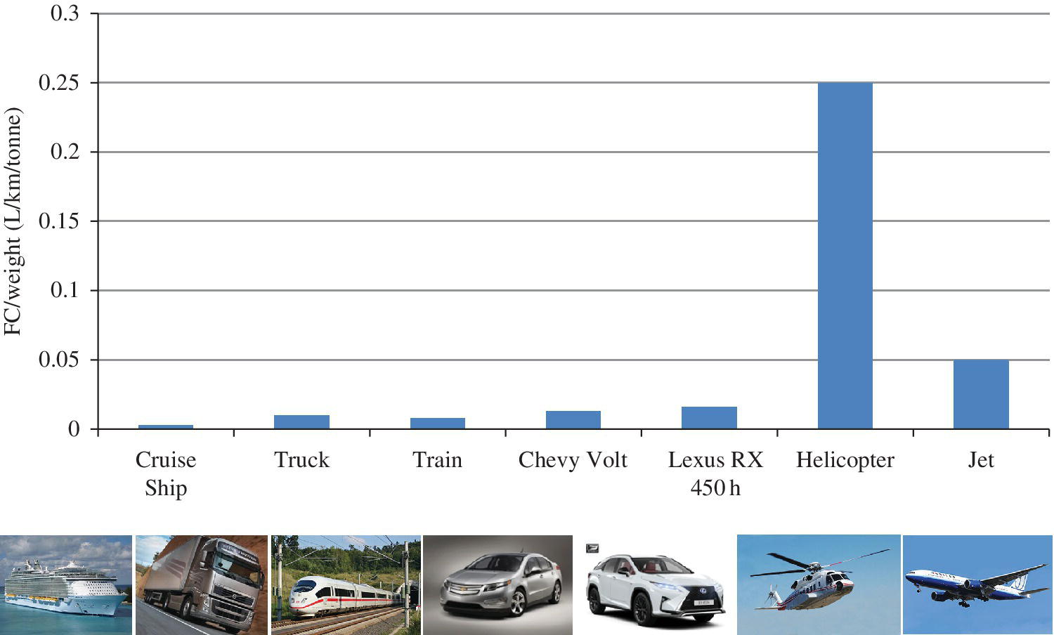
Figure 1.13 Fuel consumption per kilometer per tonne [liter/km/tonne].

The peak power‐to‐weight ratios for the various technologies are as shown in Figure 1.14. It can be seen that the commercial truck has a significantly lower power‐to‐weight ratio compared to the light‐duty sedan and SUV. This is also true for commercial buses.

Figure 1.14 Power‐to‐weight ratio for various transportation options in kW/tonne.

References

1. 1 M. Schnayerson, The Car That Could, Random House, 1996, ISBN 0‐679‐42105‐X.
2. 2 R. H. Schallenberg, “Prospects for the electric vehicle: A historical perspective,” IEEE Transactions on Education, vol. E‐23, No. 3, August 1980.
3. 3 D. Yergin, The Quest: Energy, Security, and the Remaking of the Modern World, Penguin Books, 2012, ISBN 978‐0‐241‐95777‐6.
4. 4 L. Tillemann, The Great Race: The Global Quest for the Car of the Future, Simon & Schuster, 2015.
5. 5 H. Ford (with Samuel Crowther), My Life and Work, 1923.
6. 6 A. J. Haagen‐Smit “A lesson from the Smog Capital of the World,” Proceedings of the National Academy of Sciences, October 1970.
7. 7 A. J. Haagen‐Smit, E. F. Darley, M. Zaitlin, H. Hull, and W. Noble, “Investigation on injury to plants from air pollution in the Los Angeles area,” Plant Physiology, 27 (18), 1952.
8. 8 A. Vance, Elon Musk Tesla, SpaceX, and the Quest for a Fantastic Future, HarperCollins Publishers, 2015.
9. 9 Press release, EPA's notice of violation of the Clean Air Act to Volkswagen, International Council on Clean Transportation (ICCT), Sept. 18, 2015.
10. 10 Bosch Automotive Handbook, 9th edition, Bentley Publishers, 2014.
11. 11 T. L. Brown, H. E. LeMay, B. E. Bursten, C. J. Murphy, and P. M. Woodward, Chemistry: The Central Science, 12th edition, Prentice Hall (Pearson Education).
12. 12 P. Miller, “The pulse of the planet,” National Geographic, 228 (5), November 2015.
13. 13 Department for Environment, Food and Rural Affairs, Draft Plan to Improve Air Quality in the UK, Tackling Nitrogen Dioxide in our Towns and Cities, UK overview document, September 2015.
14. 14 Website of Air Resources Board: http://www.arb.ca.gov
15. 15 Dynamometer Drive Schedules webpage of USA EPA: http://www3.epa.gov/nvfel/testing/dynamometer.htm
16. 16 Test car list data files webpage of USA EPA: https://www.epa.gov/compliance‐and‐fuel‐economy‐data/data‐cars‐used‐testing‐fuel‐economy
17. 17 US EPA, “Fuel Economy of Motor Vehicle Revisions to Improve Calculation of Fuel Economy Estimates,” December 2006.
18. 18 US EPA, “EPA Test Procedures for Electric Vehicles and Plug‐in Hybrids,” January 2015.
19. 19 Fuel economy labeling by USA EPA: http://www.fueleconomy.gov
20. 20 Fuel Economy Guide data at https://www.fueleconomy.gov/feg/download.shtml
21. 21 Natural Gas for Cars, US Department of Energy, December 2015.
22. 22 M. Wang and A. Elgowainy, Well‐to‐Wheels GHG Emissions of Natural Gas Use in Transportation: CNGVs, LNGVs, EVs, and FCVs, Argonne National Laboratory, 2014.
23. 23 GREET at http://greet.es.anl.gov
24. 24 H. C. Kim, T. J. Wallington, R. Arsenault, C. Bae, S. Ahn, and J. Lee, “Cradle‐to‐Gate Emissions from a Commercial Electric Vehicle Li‐Ion Battery: A comparative analysis,” Environmental Science and Technology, 2016, 50 (14), pp 7715–7722, doi: 10.1021/acs.est.6b00830, June 2016.
25. 25 J. Koornneef, S. Nierop, H. Saehr, and F. Wigand, “International comparison of fossil fuel efficiency and CO₂ intensity – Update 2015 Final Report,” Ecofys, 2015.
26. 26 Toyota Motor Company, Toyota’s Fuel Cell Vehicle Achievements and Pathway to Commercialization, 2010.

Further Reading

1. 1 Sony Pictures, Who Killed the Electric Car, 2006.
2. 2 N. Cawthorne, Tesla vs. Edison: The Life‐long Feud that Electrified the World, Chartwell Books, 2016.
3. 3 T. Barboza and J. Schleuss, “L.A. keeps building near freeways, even though living there makes people sick,” Los Angeles Times, March 2, 2017.
4. 4 Website of University of Southern California (USC) Environmental Health Centers, www.envhealthcenters.usc.edu.
5. 5 H. Chen, J. C. Kwong, R. Copes, K. Tu, P. J. Villeneuve, A. van Donkelaar, P. Hystad, R. V. Martin, B. J. Murray, B. Jessiman, A. S. Wilton, A. Kopp, and R. T. Burnett, “Living near major roads and the incidence of dementia, Parkinson’s disease, and multiple sclerosis: A population‐based cohort study,” The Lancet, Online January 4, 2017.

Problems

1. 1.1 Balance the following equation for the combustion of methane:
   
2. 1.2 Calculate the CO₂ emissions from the combustion of a kilogram of (a) methane and (b) diesel to verify the numbers presented in Table 1.1.
3. 1.3 The 2014 Ford Focus BEV with a 24 kWh battery pack has upstream emissions of 68 gCO₂/km (110 gCO₂/mile) in Los Angeles, 162 gCO₂/km (260 gCO₂/mile) in Detroit, and 118 gCO₂/km (190 gCO₂/mile) as an average in the United States. The gasoline 2.0 L automatic 2014 Ford Focus has total emissions of 221 gCO₂/km (356 gCO₂/mile).
   1. How many kilometers must be driven for an electric Ford Focus to result in lower carbon emissions than the gasoline Ford Focus in (a) Los Angeles, (b) Detroit, and (c) the United States, if the cradle‐to‐grave emissions of CO₂ for the electric car and gasoline car are 10,300 kg and 7,500 kg, respectively.
   2. If each car is driven for the US annual average of 21,700 km per year over eight years, determine the combined total for the cradle‐to‐grave and tailpipe and upstream emissions for the three locations using electric and gasoline.
   3. Norway has electricity emissions of about 50 times less than the United States, or about 2.5 gCO₂/km. What are the combined cradle‐grave and upstream emissions if the BEV is driven in Norway for 21,700 km per year over eight years?
   4. A representative HEV has cradle-to-grave emissions of 7,500 kg and total emissions of 118 gCO₂/km. Determine the combined total for the cradle-to-grave and tailpipe and upstream emissions for the various locations using the electric, hybrid and gasoline vehicles when driving 12,000 km per year over eight years.
   • [Ans. (i) (a) 18,300 km, (b) 47,460 km, (c) 27,180 km, (ii) LA 22,100 kg, Detroit 38,400 kg, United States 30,800 kg, gasoline 45,900 kg, (iii) Norway 10,734 kg, (iv) LA 16,828 kg, Detroit 25,852 kg, USA 21,628 kg, Norway, 10,540 kg, gasoline 28716 kg, HEV 18,828 kg]

Assignments

1. 1.1 Research the issues driving transportation emissions and fuel economy in the region where you live. What do you think are the motivating factors: security of supply, environment (GHG or pollution), and or economics?
2. 1.2 Research the well‐to‐wheel efficiencies in your region. What is the optimum mode of transport if you are to minimize carbon emissions in the overall cycle?
3. 1.3 Research the energy requirements of your home and the options for energy supply and conversion. How do these options differ from each other in terms of performance, efficiency, carbon footprint, and cost?
4. 1.4 Research the provision of electricity in your region. What are the sources? Estimate the carbon emissions in gCO₂/kWh (electrical). Reference Example 1.6.2.1.
5. 1.5 Which vehicle in the EPA database is closest to your vehicle? Which drive cycle most closely represents your driving patterns?
6. 1.6 Research the health issues affecting your community due to automotive pollution.