6
Membrane Behavior of a Laminated Composite Plate
6.1. Generalities and notations
We call laminate the superposition of a number of UD plies linked together by interfaces.
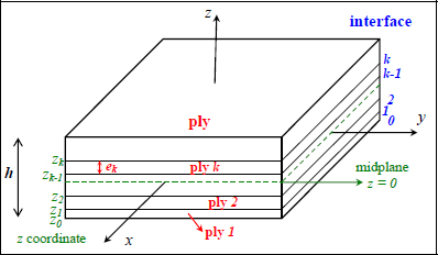
Figure 6.1. Notation of the plies within a laminate. For a color version of this figure, see www.iste.co.uk/bouvet/aeronautical2.zip
The plies are numbered from the bottom up. We note ek as the thickness of the ply k, and zk-1 and zk as the z coordinates of its lower and upper interfaces. The midplane is taken at midthickness of the laminate, and the thickness is noted as h. And for example, the draping sequence:

will be written in the following form:

Where the subscript number expresses the number of plies and S the eventual symmetry.
We will suppose that the laminate is thin, and therefore that the stress state is plane; thus, for example, the stress and strain in ply k:
which in most cases will depend on z.
Before entering into the detail of calculating a laminated plate in membrane and bending behavior, it is useful to restate what a plate model is and why is it useful. A plate model serves to transform the real 3D problem to a 2D problem (and thus makes it simpler than the initial problem).
The objective of a plate model is to regroup all the necessary information in the midplane in order to perform the required calculations using nothing but this information. Once the calculation has been done in the midplane, we can use these data to evaluate the stress and strain fields everywhere within the plate (in sum, depending on the thickness).
In practice, we will see that, knowing resultant forces, resultant moments, membrane strains and plate curvatures within the midplane, we can evaluate the stress and strain fields throughout the thickness of the plate (and, for example, apply fracture criteria). The entire constitution of the plate will then be grouped into a stiffness matrix which will link the forces (in the sense of generalized forces, in this case, resultant forces and moments) to strains (in the sense of generalized strains, in this case, membrane strains and plate curvatures). Thus, we can perform all the calculations simply using these three values (forces, strains and stiffness matrix), and once these three values have been established, we can return to the distribution of stress and strain throughout the thickness of the plate. This is evidently a similar procedure to the beam theory, where we simplify a 3D problem into a 1D problem along the neutral fiber of the beam.
6.2. Membrane behavior, bending behavior and mirror symmetry
We consider that a plate works as a membrane when all the external loadings are forces within its midplane, and its midplane does not suffer out-of-plane deformation.
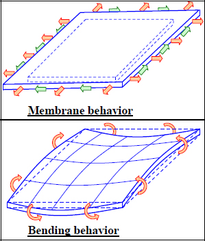
Figure 6.2. Diagram of membrane and bending behavior. For a color version of this figure, see www.iste.co.uk/bouvet/aeronautical2.zip
And conversely, a plate works under bending if the external loadings deform its midplane with out-of-plane displacements, for example, through the intermediary of moments or out-of-plane forces in this midplane.
For a laminate plate, we can demonstrate that the plate will deform with membrane displacements if the external loadings are forces (and not moments) in its midplane, and that it presents mirror symmetry.
A laminate plate presents mirror symmetry if its midplane is the symmetry plane of the draping sequence, for example:

In practice, mirror symmetry is respected for most laminates because it avoids twisting of the plate during cooldown. Indeed, laminates tend to be polymerized at high temperature, typically 120 °C for an epoxy resin, and therefore the cooldown will induce twisting if the plate does not present mirror symmetry.
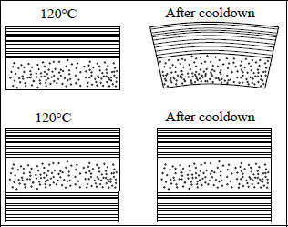
Figure 6.3. Effect of mirror symmetry during cooldown after manufacturing of the laminate
There are, nonetheless, cases where this mirror symmetry is not respected, for example, if the plate is curved (and we will then call it a shell rather than a plate), because the very shape of the structure avoids twisting. For example, for a rear propeller blade on a helicopter, the draping sequence is typically composed of two fabric plies [0/90°, 45/–45°], and the shape of the blade box and presence of foam avoids twisting during cooldown.
Mirror symmetry also allows us to avoid the coupling of membrane and bending behaviors, keeping in mind that:
- – external force loadings in the midplane only cause in-plane displacements of the midplane;
- – external moment loadings in the midplane only cause out-of-plane displacements of the midplane (in first approximation).
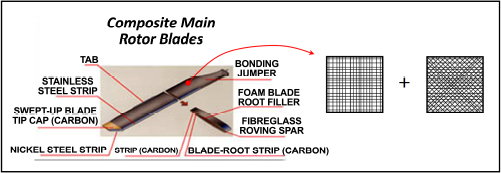
Figure 6.4. Diagram and draping sequence of a rear helicopter rotor blade [BIZ 09]. For a color version of this figure, see www.iste.co.uk/bouvet/aeronautical2.zip
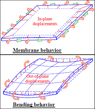
Figure 6.5. Displacements during membrane and bending loadings. For a color version of this figure, see www.iste.co.uk/bouvet/aeronautical2.zip
In the following section, we will limit ourselves to studying membrane behavior of plates with mirror symmetry, and then in the next chapter, we will look at the most common cases.
6.3. Resultant forces
Let us take a look at the stresses on a face of normal vector y:
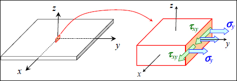
Figure 6.6. Stresses on a face of normal vector y. For a color version of this figure, see www.iste.co.uk/bouvet/aeronautical2.zip
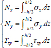
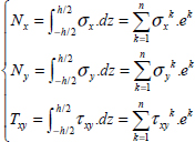
This face is subject to stresses σy along y-direction and τxy along x-direction. These stresses will, in general, depend on z, and we can sum them along z-direction in order to define a generalized force characteristic of stresses throughout the thickness of the plate:
Similarly, for a face of normal vector x subject to stresses σx along x-direction and τxy along y-direction, we define:
We can therefore define the normal resultant force along x-direction, Nx, along y-direction, Ny, and the shear resultant force, Txy:

Figure 6.7. Resultant forces for membrane behavior. For a color version of this figure, see www.iste.co.uk/bouvet/aeronautical2.zip
It is important to pay attention to the units; these resultant forces are expressed in N/mm and represent the force supported by a square plate with a one unit side. In particular, a plate with sides dx and dy is subject to the following forces:
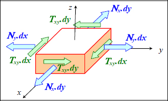
Figure 6.8. Forces on a square with sides dx and dy under membrane loading. For a color version of this figure, see www.iste.co.uk/bouvet/aeronautical2.zip
We can also demonstrate that this plate is in equilibrium no matter what the values of dx and dy are.
6.4. Displacement field, stress field and strain field
If a laminate plate presenting mirror symmetry is subject to external loading of resultant forces (Nx, Ny and Txy) in its midplane, then the displacements are planar and homogeneous along the thickness.
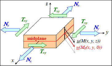
Figure 6.9. Displacement of a plate under membrane loading. For a color version of this figure, see www.iste.co.uk/bouvet/aeronautical2.zip
Where we note M(x, y, z) a random point of the plate; u(M) and v(M) its in-plane displacements; M0(x, y, 0) its projection in the midplane; and u0(M0) and v0(M0) its displacements.
We can then determine the strains, which are homogeneous through the thickness:
The strains being homogeneous throughout the thickness and the behavior being elastic and homogeneous within a single ply but different from one ply to the next, depending, among other things, on the orientation of the ply, the stresses will therefore be homogeneous within one ply, but different from one ply to the next (potentially with discontinuity among the interfaces). For instance, for ply k:
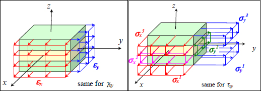
Figure 6.10. Strains and stresses in a laminate subject to membrane loading. For a color version of this figure, see www.iste.co.uk/bouvet/aeronautical2.zip
This will simplify the expression of resultant forces as follows:
With an elastic behavior law for ply k:
And therefore a relation between the resultant forces and the strains for the laminate:
With:
Again, note the units; the strains are unitless, the resultant forces are in N/mm and stiffness Aij is in N/mm.
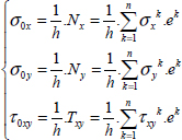
We also sometimes define the average stresses within the thickness:
Note that these stresses are just an average and do not apply to the material. Applying a fracture criterion with these average stresses would be particularly pointless.
We also define the average stiffness matrix of the laminate by:
where this time the component Aij/h represents the average stiffness in MPa.
6.5. Tension / shear coupling
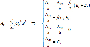
Because terms A16 and A26 are generally not 0, there is a coupling between the tension / compression behavior and the shearing behavior in the same way as for a UD subjected to stress off its orthotropic axes. However, these terms are null if the number of plies at +θ is equal to the number of plies at –θ. In practice, we often see plies at 0°, 90°, +45° and –45° and as many plies at +45° as at –45°; thus:
EXAMPLE (Laminate [0,90]S).– Consider a plate with a thickness of h = 1 mm, with a [0,90]S draping sequence (i.e. four plies of 0.25 mm thickness) made from T300/914:
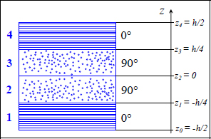
Figure 6.11. Laminate [0,90]S. For a color version of this figure, see www.iste.co.uk/bouvet/aeronautical2.zip
We then have:
And:
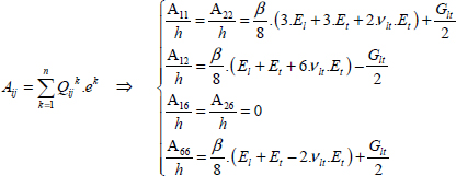
In the case where El >> Et and El >> Glt:
We obtain a material where the average modulus along x (y)-direction is due to the fibers along x (y)-direction and is equal to half the UD modulus. We also obtain a shear modulus equal to the original, which makes sense as the shear moduli of different plies are equal in (x, y). And we obtain a low Poisson’s ratio since, during tension along x (y)-direction, any shrinking along y (x)-direction will be impeded by the fibers along y (x)-direction.
Let us now study this laminate in the case of a simple tension:
then an average stress of:
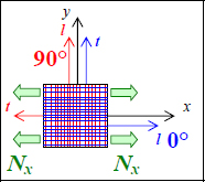
Figure 6.12. Tension of a laminate [0,90]S. For a color version of this figure, see www.iste.co.uk/bouvet/aeronautical2.zip
In order to determine the different stresses and strains in each ply, we begin by inverting the stiffness matrix  , and then multiplying it by the resultant forces to obtain the membrane strain (with Ny = Txy = 0 in this instance):
We can then determine the strains in the frame of the ply:
- – For plies 1 and 4 at 0°:
- – For plies 2 and 3 at 90°:
Use caution when using these notations; the frame (l, t) depends on the selected ply!
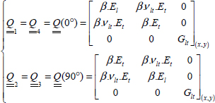
Then, by multiplying these strains with the stiffness matrix  expressed in (l, t)
(meaning it will be the same for all plies):
- – For plies 1 and 4 at 0°:
- – For plies 2 and 3 at 90°:
And, in all logic, the tension stress along x-direction is almost entirely supported by the fibers at 0°:

Figure 6.13. Strains and stresses in the plies of a laminate [0,90]S under tensile loading. For a color version of this figure, see www.iste.co.uk/bouvet/aeronautical2.zip
Note in the previous figure that we took care to present each notation in full form, specifying each time whether l and t is applied to ply at 0° or 90° (which is generally not the case, as it creates too many notations). We therefore observe that:
- – Strain εx is homogeneous throughout the thickness, as it is a membrane loading and is equal to the longitudinal strain of plies at 0°, εl0°, and to the transverse strain of plies at 90°, εt90°.
- – Strain εy is homogeneous throughout the thickness, as it is a membrane loading and is equal to the longitudinal strain of plies at 90°, εl90°, and to the transverse strain of plies at 0°, εt0°.
- – Stress σx is homogeneous for each ply (but varies from one ply to the next), as it is a membrane loading, and is equal, in plies at 0°, to longitudinal stress, σl0°, and in plies at 90°, to transverse stress σt90°. Also note that the average of σx is indeed equal to the average stress σ0x = 100 MPa, but that plies at 0° support almost twice as much loading than the average stress.
- – Stress σy is homogeneous for each ply (but varies from one ply to the next), as it is a membrane loading, and is equal, in plies at 90°, to longitudinal stress, σl90°, and in plies at 0°, to transverse stress, σt0°. Also note that the average of σy is null because the average stress along y-direction is null (σ0y = 0 MPa).
We can then trace the evolution of the moduli depending on the orientation of the laminate (Figure 6.14).
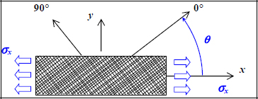
Figure 6.14. Off-axis tension of a laminate [0,90]S. For a color version of this figure, see www.iste.co.uk/bouvet/aeronautical2.zip
Where E0 = 70.7 GPa (Figure 6.15) is Young’s modulus along x-direction when θ = 0°. We obtain the maximum Young’s modulus at 0° and at 90°, and equal moduli Ex and Ey. The shear modulus has a value equal to Glt at 0° and 90° and reaches its maximum at 45°: indeed shearing induces tension / compression at ±45°. This phenomenon will be specified in the following example. The Poisson’s ratio is practically null at 0° and 90° as previously mentioned, and we can demonstrate that it is maximum and has a value of approximately 0.8 at 45°. As for the coupling coefficients, they are null at 0°, 45° and 90° thanks to the symmetries. In these three cases, the material is orthotropic (at least for its membrane behavior) and loaded along its orthotropic axes.
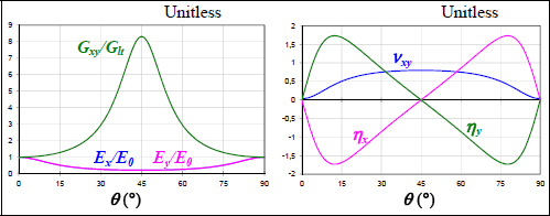
Figure 6.15. Elasticity characteristics of an off-axis laminate [0,90]S. For a color version of this figure, see www.iste.co.uk/bouvet/aeronautical2.zip
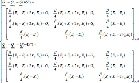
EXAMPLE (Laminate [45,–45]S).– Consider a plate with a thickness h and a [45,–45]S draping sequence.
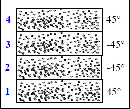
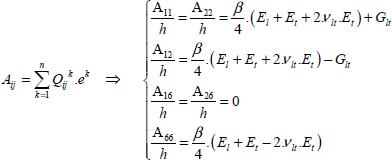
We then obtain:
And:
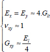
Or in the case where El >> Et and El >> Glt:
We therefore obtain a low average modulus along x (y)-direction facing the fiber modulus because loads along x (y)-direction mainly generate shear strain γlt.
Let us now study this laminate for a simple tensile loading:
Then an average stress of:
By then inverting the stiffness matrix  , we get:
Or in the coordinate systems of the plies:
- – For plies 1 and 4 at 45°:
- – For plies 2 and 3 at –45°:
Tension along x-direction will therefore be supported by tension in the fibers and shearing. Evidently, the shear stiffness is lower than the fiber stiffness, and this low stiffness will govern the stiffness of the laminate under tensile loading; stiffness that will therefore also be low and be governed by the shear modulus. This explains that Poisson’s ratio is in the order of 1, because this tension will mainly cause shear strain.
Finally, we obtain a shear modulus governed by the stiffness of the fibers and therefore far higher than the initial shear modulus. This is due to the fact that a shear stress in (x, y) will be decomposed into a tension at 45° and a compression at –45° and will therefore load the fibers at 45° and –45°.
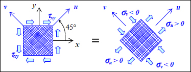
Figure 6.17. Shear stress of a 45° ply. For a color version of this figure, see www.iste.co.uk/bouvet/aeronautical2.zip
This fundamental point can be summed up as:
In order to obtain high shear stiffness, the fibers need to be placed at +45° and at –45°.
Finally, we can study the stiffness moduli of this laminate depending on the orientation of the laminate; this obviously gives us the same curves as for laminate [0,90]S offset by 45°. And we observe once again that the maximum shear modulus is at 45°.
EXAMPLE (Quasi-isotropic laminate).–
If we wish to realize a planar isotropic laminate, meaning that it presents the same behavior in all orientations (and since for manufacturing reasons, we only use plies at 0°, 90°, 45° and –45°) while respecting mirror symmetry, then we generally use the draping sequence:

We restate that using composite to realize an isotropic plate generally does not make sense as the point of composite is to adapt to the loading of the structure; this reflex to use an isotropic material is a habit that arises from metal design where plates are generally isotropic.
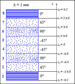
Figure 6.18. Quasi-isotropic laminate [0,45,90,–45]S. For a color version of this figure, see www.iste.co.uk/bouvet/aeronautical2.zip
We then obtain:
Then in the case where El >> Et and El >> Glt:
We will therefore have a modulus along x (y)-direction linked to the stiffness of the fibers, mainly to fibers at 0° (90°) and in part to fibers at ±45°. As for the shear modulus, it is entirely due to the fibers at ±45°. Note also that we observe the relation linking the shear modulus to Young’s modulus and Poisson’s ratio of an isotropic material:
In reality, Et and Glt are not really negligible compared to El, and these conclusions need to be nuanced.
For example, if we consider a T300/914 subject to a tensile resultant force:

Figure 6.19. Quasi-isotropic laminate [0,45,90,–45]S under tension. For a color version of this figure, see www.iste.co.uk/bouvet/aeronautical2.zip
We then obtain:
- – For plies 1 and 8 at 0°:
- – For plies 2 and 7 at 45°:
- – For plies 3 and 6 at 90°:
- – For plies 4 and 5 at –45°:
In this way, we observe that, when a quasi-isotropic laminate is loaded by an average tensile stress, the plies at 0° experience almost three times more stress (in the fiber direction), the plies at ±45° experience more or less the same stress (in the fiber direction), and the plies at 90° experience a compression stress almost equal (in absolute value). This illustrates in particular that we must always watch the notation of average stress since no plies feel it (some experience more and others less), and that it should never be used to apply a fracture criterion!
We can then trace the evolution of the moduli of a quasi-isotropic laminate depending on the orientation of the laminate:
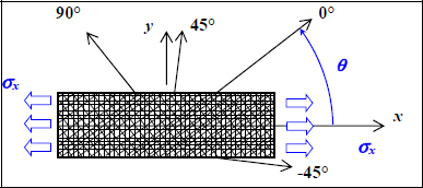
Figure 6.20. Quasi-isotropic laminate [0,45,90,–45]S under off-axis tensile loading. For a color version of this figure, see www.iste.co.uk/bouvet/aeronautical2.zip
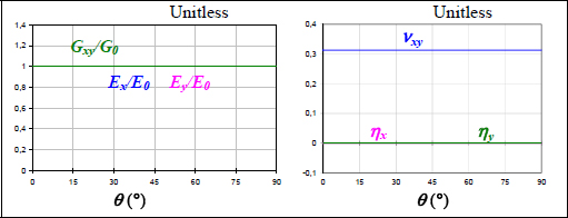
Figure 6.21. Elasticity characteristics of a quasi-isotropic laminate [0,45,90,–45]S under off-axis traction. For a color version of this figure, see www.iste.co.uk/bouvet/aeronautical2.zip
And we then get a lovely Lapalissade, i.e. that a quasi-isotropic laminate is actually isotropic. We can then wonder why we use the term quasi-isotropic and not isotropic: in the upcoming chapter, we will demonstrate that if the membrane stiffness is planar isotropic, this is not the case for the bending stiffness, and thus the use of “quasi”!


