7
Bending Behavior of a Laminated Composite Plate
7.1. Notations
The notations here will be the same as in the previous chapter:

Figure 7.1. Notation of the plies within a laminate. For a color version of this figure, see www.iste.co.uk/bouvet/aeronautical2.zip
7.2. Resultant moments
On top of resultant forces raised in the previous chapter:
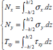
Stresses σx, σy and τxy will cause moments in the mid-plane:
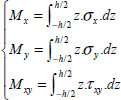

Figure 7.2. Laminate under membrane/bending loading (3D diagram). For a color version of this figure, see www.iste.co.uk/bouvet/aeronautical2.zip

Figure 7.3. Laminate under membrane and bending loading (in-plane diagram). For a color version of this figure, see www.iste.co.uk/bouvet/aeronautical2.zip
Note the units: these resultant moments are in N.mm/mm or in N and represent the moment supported by a plate with a single unit side.
Due to their definitions, Mx (My) represents the moment resulting from stress σx (σy) on a face of normal vector x (y) and is therefore directed along y (-x)-direction; Mxy is the resultant moment from stress τxy on a face of normal vector x and is therefore directed along -x-direction or by symmetry due to stress τxy on a face of normal vector y and therefore directed along y-direction.
Mx (My) represents the resultant moment of bending around y (x) and Txy the resultant moment of twisting :

Figure 7.4. The three bending/twisting resultant moments. For a color version of this figure, see www.iste.co.uk/bouvet/aeronautical2.zip
7.3. Displacement field, stress field and strain field
Consider a laminate plate presenting mirror symmetry and under external resultant moments (Mx, My and Mxy) in its mid-plane. We apply the Love–Kirschoff hypothesis: a normal vector in the mid-plane before deformation will remain a line segment perpendicular to the mid-plane after deformation.

Figure 7.5. Displacement field of a plate under bending loading. For a color version of this figure, see www.iste.co.uk/bouvet/aeronautical2.zip

Figure 7.6. Displacement field of a plate under bending loading. For a color version of this figure, see www.iste.co.uk/bouvet/aeronautical2.zip
And the displacement of any given point M(x,y,z) of the laminate can then be presented as follows:
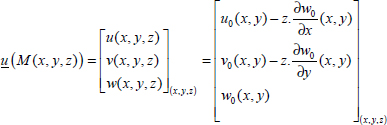
Where displacements u0(x,y) and v0(x,y) are (upon first glance) the results of the membrane loading as discussed in the previous chapter, displacement w0(x,y) is the displacement along z-direction of the mid-plane that results from bending and ∂w0/∂x (∂w0/∂y) represents the angle of rotation of the normal vector of the mid-plane along -y (x)-direction. We can then deduce the strains, which are not constant throughout the thickness as in the case of membrane loading but rather linear throughout the thickness:

Figure 7.7. Membrane and bending strains within a plate. For a color version of this figure, see www.iste.co.uk/bouvet/aeronautical2.zip
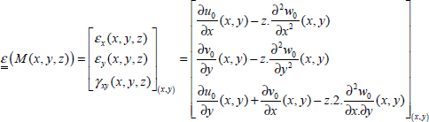
Or even:
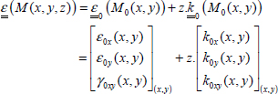
With:
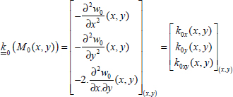
Where  0(M0(x,y)) represents the curvature of the plate defined in the mid-plane. Subsequently the information of the mid-plane, i.e. its in-plane strain and curvature, allows us to determine the strains of any given point of the plate (meaning we have successfully built a plate model).
As the strains are linear throughout the thickness and the behavior of the plies is evenly elastic within a single ply but different from one to the next, the strains are therefore linear throughout each ply with potential discontinuity in the interfaces:

Figure 7.8. Bending strain and stress within a laminate. For a color version of this figure, see www.iste.co.uk/bouvet/aeronautical2.zip
As in the case of the membrane, once we know the behavior law of a ply, we can determine the stress from the resulting strain:
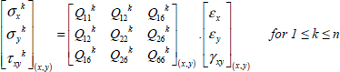
Which can be presented as follows:
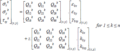
After integration according to the thickness, this allows us to determine the resultant forces and moments depending on the strain and curvature of the mid-plane:
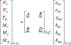
With:

Where  is the 3×3 membrane stiffness matrix that we discussed previously,
  is the 3×3 bending stiffness matrix and
  is the membrane/bending coupling matrix between the membrane behavior and the bending behavior.
Once again, note the units: the strain is unit-less, the curvature is in mm–1, the resultant force is in N/mm, the resultant moment is in N, meaning stiffness Aij is in N/mm, stiffness Bij is in N and stiffness Dij is in N.mm.
And of course:

The (membrane/bending) coupling matrix in particular implies that, when subject to loading within its mid-plane, the laminate will deform outside of its mid-plane or, subject to bending moment, it will be deformed as a membrane:

Figure 7.9. Illustration of membrane/bending coupling within a plate. For a color version of this figure, see www.iste.co.uk/bouvet/aeronautical2.zip
Coupling matrix in particular will be null for a laminate presenting mirror symmetry. Since this mirror symmetry avoids the twisting of the plate during the cooldown of the polymerization, a significant amount of laminates used in the industry present mirror symmetry.
We can also note that due to the expression of and , does not depend on the position of the plies, while depends on their respective positions. This is due to the fact that represents the in-plane stiffness of the plate and basically depends on the number of fibers in each direction, while represents the bending stiffness of the plate and depends both on the number of fibers in each direction and their position compared to the mid-plane (the further away they are, the higher the bending stiffness).
7.4. Bending/twisting coupling
As in general the terms D16 and D26 of the bending stiffness matrix are non-zero, there is a coupling between the behavior of pure bending and that of twisting. Unlike the case of the membrane, these terms are non-zero even when the number of plies at +θ is the same as the number of plies at –θ. Nonetheless, they will be null if there are only plies at 0° and at 90°, and will remain relatively low (but not null except in very specific cases) in the case where there are as many plies at +θ as there are at –θ and if these plies are bunched together in sets of two (1 at +θ and 1 at –θ).
EXAMPLE (Laminate [0,90]S).– Consider a plate with a thickness of h and a draping sequence of [0,90]S.

Figure 7.10. Laminate [0,90]S. For a color version of this figure, see www.iste.co.uk/bouvet/aeronautical2.zip
We then have:

And in the case where El>>Et and El>>Glt:

We obtain a far higher value for D11 than we do for D22, which is due to the fact that a bending moment Mx will load the 0° plies in the fiber direction, while My will load these plies in the transverse direction. The 0° plies are the furthest away from the mid-plane, meaning they are the most capable of providing bending stiffness D11. We obviously reach the same conclusion as for membrane behavior which is that to achieve a high level of stiffness, the fibers must be aligned with the loading.

Figure 7.11. Stress field within the plies of a laminate [0,90]S under bending moment Mx. For a color version of this figure, see www.iste.co.uk/bouvet/aeronautical2.zip

Figure 7.12. Stress field within the plies of a laminate [0,90]S under bending moment My. For a color version of this figure, see www.iste.co.uk/bouvet/aeronautical2.zip

Figure 7.13. Stress field within the plies of a laminate [0,90]S under twisting moment Mxy. For a color version of this figure, see www.iste.co.uk/bouvet/aeronautical2.zip
You should note that in the previous figure, the direction of stresses τxy should be along x (y)-direction for a face of normal vector y (x), which is not the case in the diagram as that would render it unreadable (thus the dotted lines).
The low value of D12 translates the coupling between directions x and y that exists thanks to the effect of the resin. Similarly, D66 is low and is only due to the shear stiffness and therefore the resin. Lastly, D16 and D26 are null as there are no plies at ±45°.
For example, if we consider a T300/914 subjected to:


Figure 7.14. Laminate [0,90]S. For a color version of this figure, see www.iste.co.uk/bouvet/aeronautical2.zip
We then have:

And we then calculate the strain field from:


Figure 7.15. Strain field within the plies of a laminate [0,90]S under bending moment Mx. For a color version of this figure, see www.iste.co.uk/bouvet/aeronautical2.zip
Thus:
- – For ply 1 at 0°, the value is maximum (in absolute value) in –h/2 and is:

- – For ply 2 at 90°, the value is maximum (in absolute value) in –h/4 and is:

- – For ply 3 at 90°, the value is maximum (in absolute value) in –h/4 and is:

- – For ply 4 at 0°, the value is maximum (in absolute value) in –h/2 and is:

EXAMPLE (Laminate [45,–45]S).– Consider a plate with a thickness of h and a draping sequence [45,–45]S.

Figure 7.16. Laminate [45,-45]S. For a color version of this figure, see www.iste.co.uk/bouvet/aeronautical2.zip
We then have:

In the case where El>>Et and El>>Glt:

Due to symmetry, D11 and D22 are equal and have relatively high values, as they are mainly due to the loading applied to 45° fibers. The values, however, remain below that of D11 for [0,90]S as the fibers are not aligned with the stress induced by bending. The twisting stiffness D66 is also relatively high since this loading (Mxy) will also load the fibers. Lastly, the coupling term between bending along x-direction and the one along y-direction, D12, as well as the terms for the coupling between bending and twisting will be relatively high for the same reasons.
EXAMPLE (Quasi-isotropic laminate).– Consider a plate with a thickness of h and a draping sequence [0,45,90,-45]S

Figure 7.17. Quasi-isotropic laminate [0,45,90,-45]S. For a color version of this figure, see www.iste.co.uk/bouvet/aeronautical2.zip
We then have:

In the case where El>>Et and El>>Glt:

We then have a high value for D11 thanks to the stiffness of the 0° fibers loaded along their direction by a moment Mx, a lower value D22 because the 90° plies are closer to the mid-plane, and a low value D12 as it is a result of the resin.
We can also question the isotropy of this laminate, indeed, in the previous chapter, we saw that the membrane behavior of this laminate was isotropic in the plane. If we trace, for instance, D11/h3 according to the θ-orientation by taking the characteristics of the aforementioned T300/914, we observe a considerable variation of D11:

Figure 7.18. Quasi-isotropic laminate [0,45,90,-45]S under off-axis loading. For a color version of this figure, see www.iste.co.uk/bouvet/aeronautical2.zip

Figure 7.19. Elastic bending characteristic D11 of a quasi-isotropic laminate [0,45,90,-45]S under off-axis loading
The maximum value of D11 is reached for a value close to 0° (or 180°, which is the same thing), meaning that the fibers of the furthest plies from the mid-plane, i.e. the ones at 0°, are directly loaded in their direction. Nonetheless, here the stiffness of the other plies, and in particular that of those at 45°, is obviously non-negligible. Similarly, the minimum value is obtained for a value close to 90° but not for 90°.
We can therefore once again conclude that in order to obtain a high bending stiffness, the fibers that are furthest from the mid-plane must be loaded along their direction.
Lastly, we note that the quasi-isotropic laminate is not completely isotropic, unlike the case of an aluminum plate:

The most common case in the aeronautical field, where a high bending stiffness is desired, is the case of buckling. Indeed, we can show (see Chapter 12) that the resistance to buckling of a plate is directly linked to its bending stiffness. It is important not to forget that the resistance to buckling of a laminate plate said to be “quasi-isotropic” is not isotropic! This isotropic designation comes from the membrane stiffness.