Chapter 3

Going the Distance with Speed and Acceleration

IN THIS CHAPTER

Getting up to speed on displacement

Examining different kinds of speed

Introducing acceleration

Linking acceleration, time, and displacement

Connecting speed, acceleration, and displacement

There you are in your Formula 1 racecar, speeding toward glory. You have the speed you need, and the pylons are whipping past on either side. You’re confident that you can win, and coming into the final turn, you’re far ahead. Or at least you think you are. It seems that another racer is also making a big effort, because you see a gleam of silver in your mirror. You get a better look and realize that you need to do something — last year’s winner is gaining on you fast.

It’s a good thing you know all about velocity and acceleration. With such knowledge, you know just what to do: You floor the gas pedal, accelerating out of trouble. Your knowledge of velocity lets you handle the final curve with ease. The checkered flag is a blur as you cross the finish line in record time. Not bad. You can thank your understanding of the issues in this chapter: displacement, speed, and acceleration.

You already have an intuitive feeling for what I discuss in this chapter, or you wouldn’t be able to drive or even ride a bike. Displacement is all about where you are, speed is all about how fast you’re going, and anyone who’s ever been in a car knows about acceleration. These forces concern people every day, and physics has made an organized study of them. Knowledge of these forces has allowed people to plan roads, build spacecraft, organize traffic patterns, fly, track the motion of planets, predict the weather, and even get mad in slow-moving traffic jams.

Understanding physics is all about understanding movement, and that’s the topic of this chapter. Time to move on.

From Here to There: Dissecting Displacement

When something moves from point A to point B, displacement takes place in physics terms. In plain English, displacement is a distance. Say, for example, that you have a fine new golf ball that’s prone to rolling around by itself, shown in Figure 3-1. This particular golf ball likes to roll around on top of a large measuring stick. You place the golf ball at the 0 position on the measuring stick, as you see in Figure 3-1, diagram A.

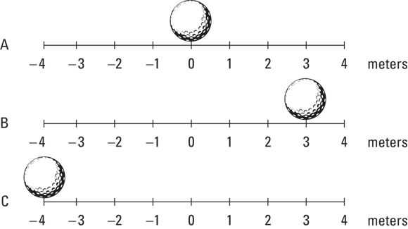
FIGURE 3-1: Examining displacement with a golf ball.

The golf ball rolls over to a new point, 3 meters to the right, as you see in Figure 3-1, diagram B. The golf ball has moved, so displacement has taken place. In this case, the displacement is just 3 meters to the right. Its initial position was 0 meters, and its final position is at meters.

In physics terms, you often see displacement referred to as the variable s (don’t ask me why). In this case, s equals 3 meters.

Scientists, being who they are, like to go into even more detail. You often see the term , which describes initial position (alternatively referred to as ; the i stands for initial). And you may see the term used to describe final position. In these terms, moving from diagram A to diagram B in Figure 3-1, is at the 0-meter mark and is at meters. The displacement, s, equals the final position minus the initial position:

Displacements don’t have to be positive; they can be zero or negative as well. Take a look at Figure 3-1, diagram C, where the restless golf ball has moved to a new location, measured as meters on the measuring stick. What’s the displacement here?

Examining axes

Motion that takes place in the world isn’t always linear, like the golf ball shown in Figure 3-1. Motion can take place in two or three dimensions. And if you want to examine motion in two dimensions, you need two intersecting meter sticks, called axes. You have a horizontal axis — the x-axis — and a vertical axis — the y-axis. (For three-dimensional problems, watch for a third axis — the z-axis — sticking straight up out of the paper.)

Take a look at Figure 3-2, where a golf ball moves around in two dimensions. It starts at the center of the graph and moves up to the right.

FIGURE 3-2: As you know from your golf game, objects don’t always move in a linear fashion.

In terms of the axes, the golf ball moves to meters on the x-axis and meters on the y-axis, which is represented as the point (4, 3); the x measurement comes first, followed by the y measurement: (x, y).

So what does this mean in terms of displacement? Well, it turns out that displacement is actually a vector (see Chapter 2 for details about vectors). To find the displacement vector, you need to find its components. The change in the x position, (, the Greek letter delta, means “change in”), is equal to the final x position minus the initial x position. If the golf ball starts at the center of the graph — the origin of the graph, location (0, 0) — you have a change in the x location of

The change in the y location is

So the displacement vector is:

Measuring speed

In the previous sections, you examine the motion of objects across one and two dimensions. But there’s more to the story of motion than just the actual movement. When displacement takes place, it happens in a certain amount of time, which means that it happens at a certain speed. How long does it take the ball in Figure 3-1, for example, to move from its initial to its final position? If it takes 12 years, that makes for a long time before the figure was ready for this book. Now, 12 seconds? Sounds more like it.

Measuring how fast displacement happens is what the rest of this chapter is all about. Just as you can measure displacement, you can measure the difference in time from the beginning to the end of the motion, and you usually see it written like this:

Here, is the final time, and is the initial time. The difference between these two is the amount of time it takes something to happen, such as a golf ball moving to its final destination. Scientists want to know all about how fast things happen, and that means measuring speed.

The Fast Track to Understanding Speed and Velocity

You may already have the conventional idea of speed down pat, assuming you speak like a scientist:

For example, if you travel distance s in a time t, your speed, v, is

The variable v really stands for velocity, but true velocity also has a direction associated with it, which speed does not. For that reason, velocity is a vector and you usually see it represented as v. Vectors have both a magnitude and a direction, so with velocity, you know not only how fast you’re going but also in what direction. Speed is only a magnitude (if you have a certain velocity vector, in fact, the speed is the magnitude of that vector), so you see it represented by the term v (not in bold).

Phew, that was easy enough, right? Technically speaking (physicists love to speak technically), speed is the change in position divided by the change in time, so you can also represent it like this, if, say, you’re moving along the x-axis:

Speed can take many forms, which you find out about in the following sections.

How fast am I right now? Instantaneous speed

You already have an idea of what speed is; it’s what you measure on your car’s speedometer, right? When you’re tooling along, all you have to do to see your speed is look down at the speedometer. There you have it: 75 miles per hour. Hmm, better slow it down a little — 65 miles per hour now. You’re looking at your speed at this particular moment. In other words, you see your instantaneous speed.

Instantaneous speed is an important term in understanding the physics of speed, so keep it in mind. If you’re going 65 mph right now, that’s your instantaneous speed. If you accelerate to 75 mph, that becomes your instantaneous speed. Instantaneous speed is your speed at a particular instant of time. Two seconds from now, your instantaneous speed may be totally different.

Staying steady: Uniform speed

What if you keep driving 65 miles per hour forever? You achieve uniform speed in physics (also called constant speed). Uniform motion is the simplest speed variation to describe, because the speed never changes.

Changing your speed: Nonuniform motion

Nonuniform motion varies over time; it’s the kind of speed you encounter more often in the real world. When you’re driving, for example, you change speed often, and your changes in speed come to life in an equation like this, where is your final speed and is your original speed:

The last part of this chapter is all about acceleration, which occurs in nonuniform motion.

Doing some calculations: Average speed

Say that you want to pound the pavement from New York to Los Angeles to visit your uncle’s family, a distance of about 2,781 miles. If the trip takes you four days, what was your speed?

Speed is the distance you travel divided by the time it takes, so your speed for the trip would be

Okay, you calculate 695.3, but 695.3 what?

This solution divides miles by days, so you come up with 695.3 miles per day. Not exactly a standard unit of measurement — what’s that in miles per hour? To find out, you want to cancel “days” out of the equation and put in “hours.” Because a day is 24 hours, you can multiply this way (note that “days” cancel out, leaving miles over hours, or miles per hour):

You go 28.97 miles per hour. That’s a better answer, although it seems pretty slow, because when you’re driving, you’re used to going 65 miles per hour. You’ve calculated an average speed over the whole trip, obtained by dividing the total distance by the total trip time, which includes nondriving time.

Contrasting average speed and instantaneous speed

Average speed differs from instantaneous speed (unless you’re traveling in uniform motion, in which case your speed never varies). In fact, because average speed is the total distance divided by the total time, it may be very different from your instantaneous speed.

During a trip from New York to L.A., you may stop at a hotel several nights. While you sleep, your instantaneous speed is 0 miles per hour; yet, even at that moment, your average speed is still 28.97 miles per hour (see the previous section for this calculation). That’s because you measure average speed by dividing the whole distance, 2,781 miles, by the time the trip takes, 4 days.

Average speed also depends on the start and end points. Say, for example, that while you’re driving in Ohio on your cross-country trip, you want to make a detour to visit your sister in Michigan after you drop off a hitchhiker in Indiana. Your travel path may look like the straight lines in Figure 3-3 — first 80 miles to Indiana and then 30 miles to Michigan.

FIGURE 3-3: Traveling detours provide variations in average speed.

If you drive 55 miles per hour, and you have to cover , it takes you 2 hours. But if you calculate the speed by taking the distance between the starting point and the ending point, 85.4 miles as the crow flies, you get

You’ve calculated your average speed along the dotted line between the start and end points of the trip, and if that’s what you really want to find, no problem. But if you’re interested in your average speed along either of the two legs of the trip, you have to measure the time it takes for a leg and divide by length of that leg to get the average speed for that part of the trip.

If you move at a uniform speed, your task becomes easier. You can look at the whole distance traveled, which is , not just 85.4 miles. And 110 miles divided by 2 hours is 55 miles per hour, which, because you travel at a constant speed, is your average speed along both legs of the trip. In fact, because your speed is constant, 55 miles per hour is also your instantaneous speed at any point on the trip.

When considering motion, speed is not the only thing that counts; direction matters too. That’s why velocity is important, because it lets you record an object’s speed and direction. Pairing speed with direction enables you to handle cases like cross-country travel, where the direction can change.

Speeding Up (or Slowing Down): Acceleration

As with speed, you already know the basics about acceleration. Acceleration is how fast your velocity changes. When you pass a parking lot’s exit and hear squealing tires, you know what’s coming next — someone is accelerating to cut you off. And sure enough, the jerk appears right in front of you, missing you by inches. After he passes, he slows down, or decelerates, right in front of you, forcing you to hit your brakes to decelerate yourself. Good thing you know all about physics.

Defining our terms

In physics terms, acceleration, a, is the amount by which your velocity changes in a given amount of time, or

Given the initial and final velocities, and , and initial and final times over which your velocity changes, and , you can also write the equation like this:

Recognizing positive and negative acceleration

Don’t let someone catch you on the wrong side of a numeric sign. Accelerations, like speeds, can be positive or negative, and you have to make sure you get the sign right. If you decelerate to a complete stop in a car, for example, your original speed was positive and your final speed is 0, so the acceleration is negative.

Acceleration, like speed, has a sign, as well as units.

Also, don’t get fooled into thinking that a negative acceleration (deceleration) always means slowing down or that a positive acceleration always means speeding up. For example, take a look at the ball in Figure 3-4, which is happily moving in the negative direction in diagram A. In diagram B, the ball is still moving in the negative direction, but at a slower speed.

FIGURE 3-4: The golf ball is traveling in the negative direction, but with a positive acceleration, so it slows down.

Because the ball’s negative speed has decreased, the acceleration is positive during the speed decrease. In other words, to slow its negative speed, you have to add a little positive speed, which means that the acceleration is positive.

The sign of the acceleration tells you how the speed is changing. A positive acceleration says that the speed is increasing in the positive direction, and a negative acceleration tells you that the speed is increasing in the negative direction.

Looking at average and instantaneous acceleration

Just as you can examine average and instantaneous speed, you can examine average and instantaneous acceleration. Average acceleration is the ratio of the change in velocity and the change in time. You calculate average acceleration, also written as , by taking the final velocity, subtracting the original velocity, and dividing the result by the total time (final time minus the original time):

This equation gives you an average acceleration, but the acceleration may not have been that average value all the time. At any given point, the acceleration you measure is the instantaneous acceleration, and that number can be different from the average acceleration. For example, when you first see red flashing police lights behind you, you may jam on the brakes, which gives you a big deceleration. But as you coast to a stop, you lighten up a little, so the deceleration is smaller; however, the average acceleration is a single value, derived by dividing the overall change in velocity by the overall time.

Accounting for uniform and nonuniform acceleration

Acceleration can be uniform or nonuniform. Nonuniform acceleration requires a change in acceleration. For example, when you’re driving, you encounter stop signs or stop lights often, and when you decelerate to a stop and then accelerate again, you take part in nonuniform acceleration.

Other accelerations are very uniform (in other words, unchanging), such as the acceleration due to gravity on the surface of the Earth. This acceleration is 9.8 meters per second² downward, toward the center of the earth, and it doesn’t change. (If it did, plenty of people would be pretty startled.)

Bringing Acceleration, Time, and Displacement Together

You deal with four quantities of motion in this chapter: acceleration, speed, time, and displacement. To relate displacement and time in order to get speed (in one dimension), you use this standard equation:

To find the acceleration in one dimension from speed and time, you use this equation:

But both equations go only one level deep, relating speed to displacement and time and acceleration to speed and time. What if you want to relate acceleration to displacement and time?

Say, for example, you give up your oval-racing career to become a drag racer in order to analyze your acceleration down the dragway. After a test race, you know the distance you went — 0.25 mile, or about 402 meters — and you know the time it took — 5.5 seconds. So, how hard was the kick you got — the acceleration — when you blasted down the track? Good question. You want to relate acceleration, time, and displacement; speed isn’t involved.

You can derive an equation relating acceleration, time, and displacement. To make this step simpler, this derivation doesn’t work in terms of . When you’re slinging around algebra, you may find it easier to work with single quantities like v rather than , if possible. You can usually turn v into later, if necessary.

Locating not-so-distant relations

You relate acceleration, distance, and time by messing around with the equations until you get what you want. Displacement equals average speed multiplied by time:

You have a starting point. But what’s the average speed during the drag race from the previous section? You started at 0 and ended up going pretty fast. Because your acceleration was constant, your speed increased in a straight line from 0 to its final value.

On average, your speed was half your final value, and you know this because there was constant acceleration. Your final speed was

Okay, you can find your final speed, which means your average speed (because it went up in a straight line) was

So far, so good. Now you can plug this average speed into the equation and get

And because you know that , you can get

And this becomes

You can also put in rather than just plain t:

Congrats! You’ve worked out one of the most important equations you need to know when you work with physics problems relating acceleration, displacement, time, and speed.

Equating more speedy scenarios

What if you don’t start off at zero speed, but you still want to relate acceleration, time, and displacement? What if you’re going 100 miles per hour? That initial speed would certainly add to the final distance you go. Because distance equals speed multiplied by time, the equation looks like this (don’t forget that this assumes the acceleration is constant):

Quite a mouthful. As with other long equations, I don’t recommend you memorize the extended forms of these equations unless you have a photographic memory. It’s tough enough to memorize

If you don’t start at 0 seconds, you have to subtract the starting time to get the total time the acceleration is in effect.

If you don’t start at rest, you have to add the distance that comes from the initial velocity into the result as well. If you can, it really helps to solve problems by using as much common sense as you can so you have control over everything rather than mechanically trying to apply formulas without knowing what the heck is going on, which is where errors come in.

So, what was your acceleration as you drove the drag racer I introduced in the last couple sections? Well, you know how to relate distance, acceleration, and time, and that’s what you want — you always work the algebra so that you end up relating all the quantities you know to the one quantity you don’t know. In this case, you have

You can rearrange this equation with a little algebra; just divide both sides by and multiply by 2 to get

Great. Plugging in the numbers, you get

Okay, . What’s that in more understandable terms? The acceleration due to gravity, g, is , so this is about 2.7 g.

Putting Speed, Acceleration, and Displacement Together

Impressive, says the crafty physics textbook, you’ve been solving problems pretty well so far. But I think I’ve got you now. Imagine you’re a drag racer for an example problem. I’m going to give you only the acceleration — 26.6 meters per second² — and your final speed — 146.3 meters per second. With this information, I want you to find the total distance traveled. Got you, huh? “Not at all,” you say, supremely confident. “Just let me get my calculator.”

You know the acceleration and the final speed, and you want to know the total distance it takes to get to that speed. This problem looks like a puzzler because the equations in this chapter have involved time up to this point. But if you need the time, you can always solve for it. You know the final speed, , and the initial speed, (which is zero), and you know the acceleration, a. Because

you know that

Now you have the time. You still need the distance, and you can get it this way:

The first term drops out, because , so all you have to do is plug in the numbers:

In other words, the total distance traveled is 402 meters, or a quarter mile. Must be a quarter-mile racetrack.

If you’re an equation junkie (and who isn’t?), you can make this step simpler on yourself with a new equation, the last one for this chapter. You want to relate distance, acceleration, and speed. Here’s how it works; first, you solve for the time:

Because , and when the acceleration is constant, you can get

Substituting for the time, you get

After doing the algebra, you get

Moving the 2a to the other side of the equation, you get an important equation of motion:

Whew. If you can memorize this one, you’re able to relate velocity, acceleration, and distance. You can now consider yourself a motion master.