FIGURE 8.1 GPS system satellite constellation.
In this chapter, I will discuss a GPS-based location system that is easily carried aloft by an Elev-8 or other quadcopters with similar lifting capacity. The system will transmit its data to a ground station where the quadcopter’s position, speed, course, and altitude will be visible on a small display. The coordinates could also be entered into a laptop in order to display the quadcopter’s position in the Google Earth application. This system, together with the First-Person Video system described in the next chapter will be used to accurately determine the quadcopter’s location and to view the environment in real time.
We will begin with a short history of the Global Positioning System (GPS), and follow that with a detailed explanation of how GPS systems generally function. Then I will focus on the quadcopter’s GPS receiver and the development of a real-time display.
The GPS is a satellite system that was initially deployed in the early 1970s by the U.S. Department of Defense (DoD) to provide military users with precise location and time synchronization services. Civilian users could also access the system, but its services to civilian users were purposefully degraded by the DoD to avoid any risk that it could be of help to the country’s enemies. This purposeful degradation was lifted by order of President Regan in the 1980s to allow civilians full and accurate GPS services.
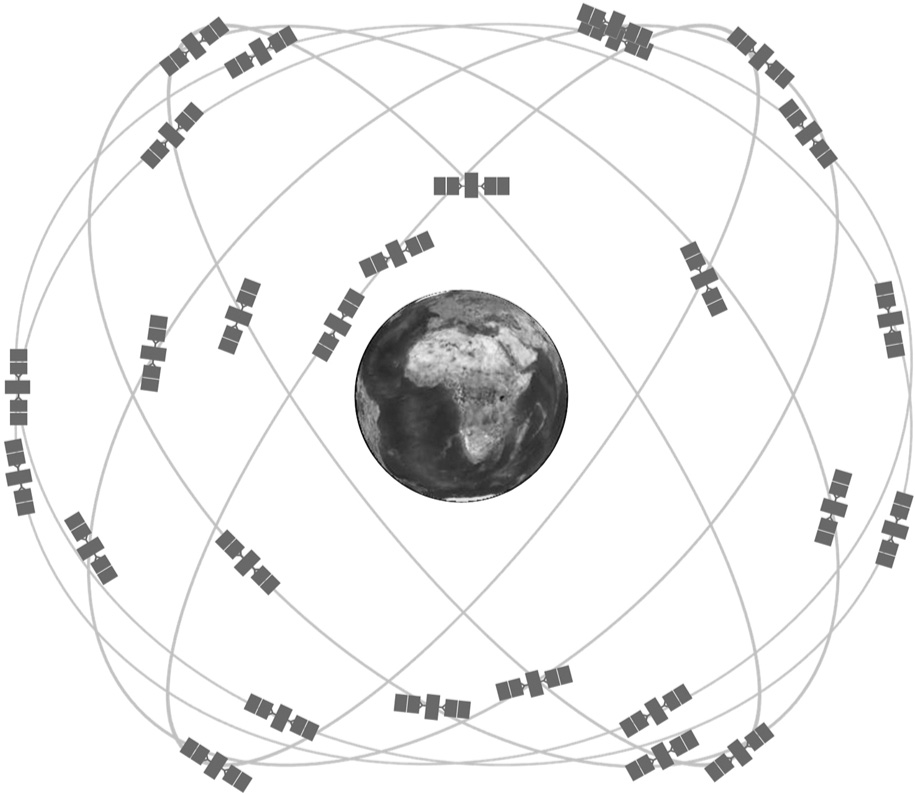
The current GPS system has 32 satellites in high orbits over the earth. Figure 8.1 shows a representative diagram of the satellite constellation. The satellite orbits have been carefully designed to allow for a minimum of six satellites to be in the instantaneous field of view of a GPS user who is located anywhere on the surface of the earth. A minimum of four satellites must be viewed in order to obtain a location fix, as you will learn in the GPS basics section.
Several other GPS systems are also deployed:
GLONASS—The Russian GPS
Galileo—The European GPS
Compass—The Chinese GPS
IRNSS—The Indian Regional Navigation Satellite System
I will be using the U.S. GPS system because vendors have made many inexpensive receivers for that system available for purchase. All receivers function essentially in the same way and conform to the National Marine Electronics Association (NMEA) standard discussed in a later section.
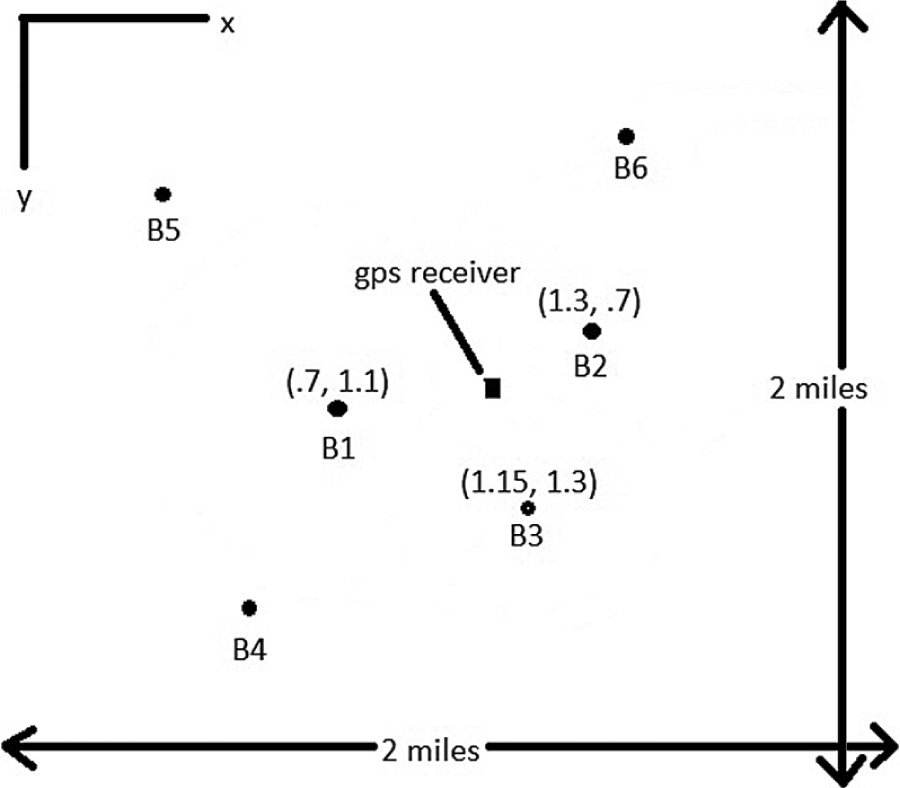
I made up an analogous, fictional, position-location system to help explain how the GPS system functions. First, imagine a two-mile by two-mile land area where this system is set up. The land terrain contains gently rolling hills, each no more than 30 feet in height. The subject, using a special GPS receiver, may be located anywhere within this area. Also located in this area are six 100-ft towers, each containing a beacon. The beacon atop each tower briefly flashes a light and simultaneously emits a loud burst of sound. Each beacon also emits the light and sound pulses once a minute but at a specific time within the minute. Beacon one (B1) emits at the start of the minute, beacon two (B2) at 10 seconds past the start of the minute, beacon three (B3) at 10 seconds later, and so on for the remaining beacons.
It is also critical that the GPS receiver have a line of sight to each beacon and also that the position of each beacon is recorded in an embedded database that is also constantly available to the receiver. The beacon positions B1 through B3 are recorded in x and y coordinates in terms of miles from the origin, which is located in the upper left hand corner of the test area, as shown in Figure 8.2.
The actual position determination happens in the following fashion:
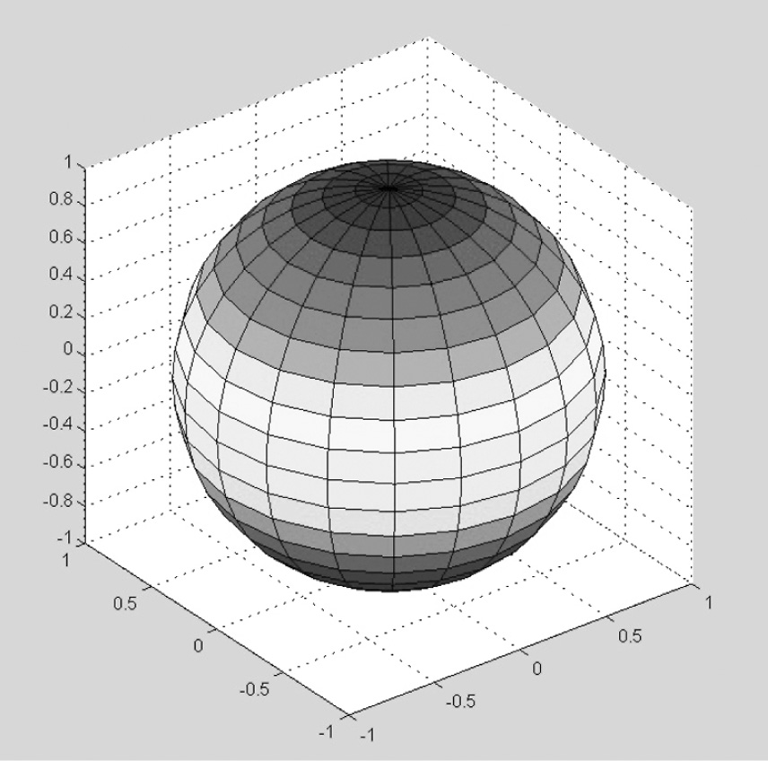
• At the start of the minute, B1 flashes, and the receiver starts a timer that stops when the sound pulse is received. Since the light flash is essentially instantaneous, the time interval is proportional to the distance from the beacon. Since sound travels nominally at 1100 feet/s (second) in air, a 5-second delay would represent a 5500-ft distance. The receiver must then be located somewhere on a 5500-ft radius sphere that is centered on B1. Figure 8.3 illustrates this abstraction in a graphical representation taken from a Mathworks Matlab application.
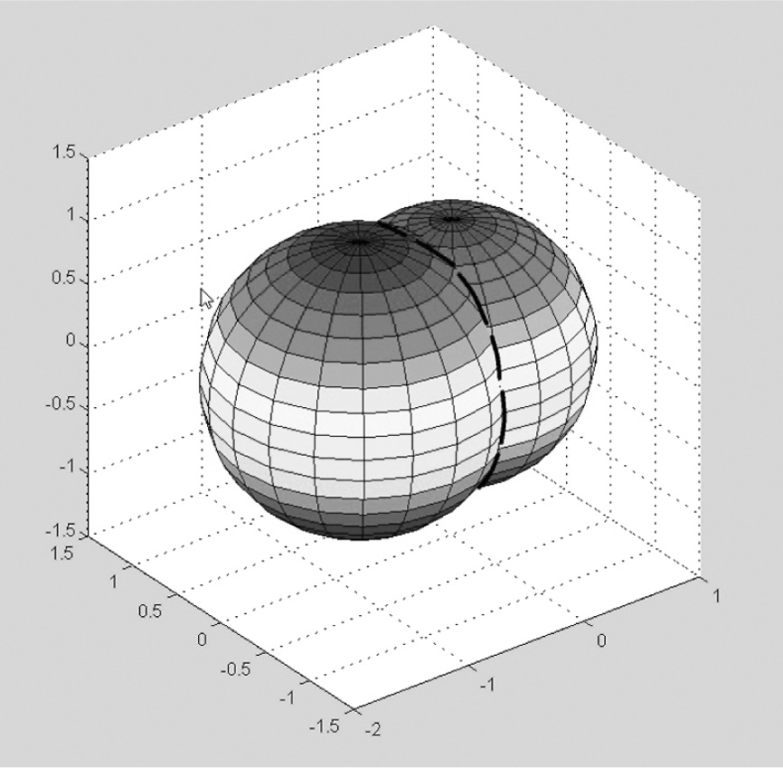
• B2 flashes next. Suppose it takes 4 seconds for the B2 sound pulse to reach the GPS receiver. This delay represents a 4400-ft sphere centered on B2. The B1 sphere and B2 sphere are shown intersecting in Figure 8.4. The heavily dashed line represents the portion of the circle that is the intersection of these two spheres. The receiver must lie somewhere on this circle. The circle is a straight line when observed in a planar or perpendicular view. There is still, however, some doubt or uncertainty as to where the receiver is located on the circle. Thus, another beacon is still needed to resolve the uncertainty.
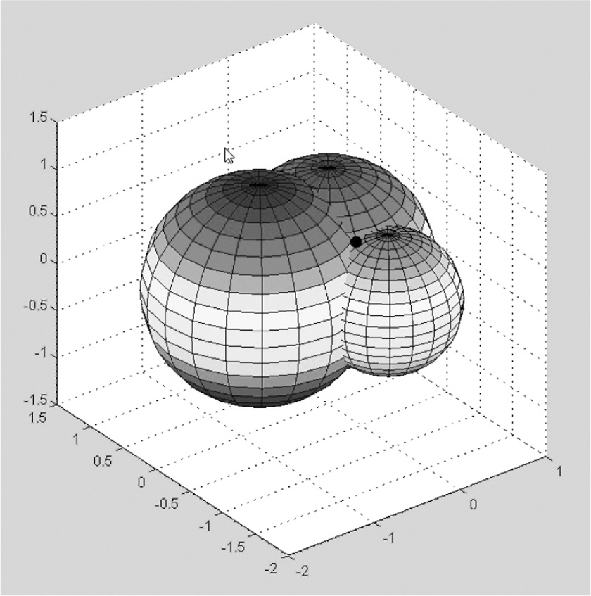
• B3 flashes next, and suppose it takes 3 seconds for the B3 sound pulse to reach the GPS receiver. This delay represents a 3300-ft sphere centered on B3. The B1, B2, and B3 spheres are shown intersecting in Figure 8.5. The receiver must be located at the star shown in the figure. In reality, it could be at either a high or low point since the third sphere intersects the two other spheres at two points. The receiver position has now been fixed with regard to x and y coordinates but not the third, or z coordinate. Guess what? Now you need a fourth beacon to resolve whether the receiver is at the high or low point. I am not going to go through the whole process again; I think you have figured it out by now.
• Figure 8.5 shows a plane view of all three spheres with the GPS receiver position shown. You can think of it as a horizontal slice taken at z = 0, as shown in Figure 8.6.
In summary, it takes a minimum of three beacons to determine the x and y coordinates and a fourth beacon to fix the z coordinate. Now translate beacons to satellites and x, y, and z coordinates to latitude, longitude, and altitude, and you have the basics of the real GPS system.
The satellites transmit digital microwave radio frequency (RF) signals that contain both identity and timing components that a real GPS receiver will use to calculate its position and altitude. The counterpart to the embedded database mentioned in my example is called an ephemeris, or celestial almanac, that contains all the data necessary for the receiver to calculate a particular satellite’s orbital position. All GPS satellites are in high earth orbits (as mentioned in the history section) and are constantly changing position. This movement requires the receiver to use a dynamic means for acquiring their position fix, which, in turn, is provided by the ephemeris. This is one reason why it may take a while for a real GPS receiver to establish a lock, as it must go through a considerable amount of data calculations to determine actual satellite positions within its field of view.
In my example, the radii of the “location spheres” are determined by the receiver using extremely precise timing signals contained in the satellite transmissions. Each satellite contains an atomic clock to generate these clock signals. All satellite clocks are constantly synchronized and updated from earth-based ground stations. These constant updates are needed to maintain GPS accuracy, which would naturally degrade because of two relativistic effects. The best way to describe the first effect is to retell the paradox of the space-travelling twin.
Imagine a set of two twins, (male, female—doesn’t matter) one of whom is slated to take a trip on a fast starship to our closest neighboring star, Alpha Centauri. This round trip will take about ten years travelling at nearly the speed of light. The other twin will stay on Earth awaiting the return of his/her sibling. The twin in the space ship will accelerate very close to light speed and will patiently wait the ten years it will take, according to the clock in the ship, to make the round trip. According to Professor Einstein, if the travelling twin could view a clock on Earth he/she would observe time going by more quickly than it did in the spaceship. This effect is part of the theory of special relativity and, more specifically, is called time dilation. If the twin on Earth could view the clock in the spaceship, he/she would see it turning at a much slower rate than the earthbound clock. Imagine what happens when the travelling twin returns and finds that he/she is only ten years older but that the earthbound twin is 50 years older due to time dilation. The space twin will have time travelled a net 40 years into Earth’s future by taking the ten-year space trip!
The second effect is more complex than time dilation. I will simply state what it is. According to Einstein’s theory of general relativity, objects located close to massive objects, such as the earth, will have their clocks moving slower as compared to objects that are further away from the massive objects. This effect is due to the curvature of the space-time continuum predicted and experimentally verified by the general relativity theory.
Now back to the GPS satellites that are orbiting at 14,000 kilometers per hour (km/h), while the earth is rotating at a placid 1,666 km/h. The relativistic time dilation due to the speed differences is approximately –7 µsec/day, while the difference due to space-time is + 45 µsec/day for a net satellite clock gain of 38 µsec/day. While this error is nearly infinitesimal on a short-term basis, it would be very noticeable over a day. The total daily, accumulated error would amount to a position error of 10 km or 6.2 miles (mi), essentially making GPS useless. That is why the earth ground stations constantly update and synchronize the GPS satellite atomic clocks.
NOTE: As a point of interest, the atomic clocks within the GPS satellites are deliberately slowed prior to being launched to counteract the relativistic effects described earlier. Ground updates are still needed to ensure that the clocks are synchronized to the desired one nanosecond of accuracy.
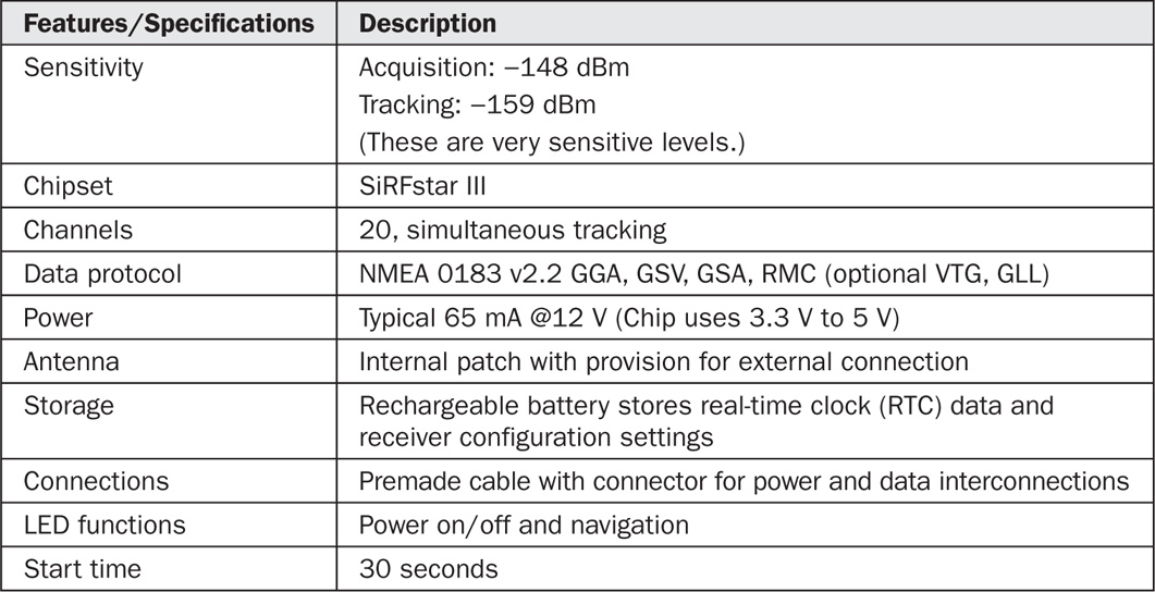
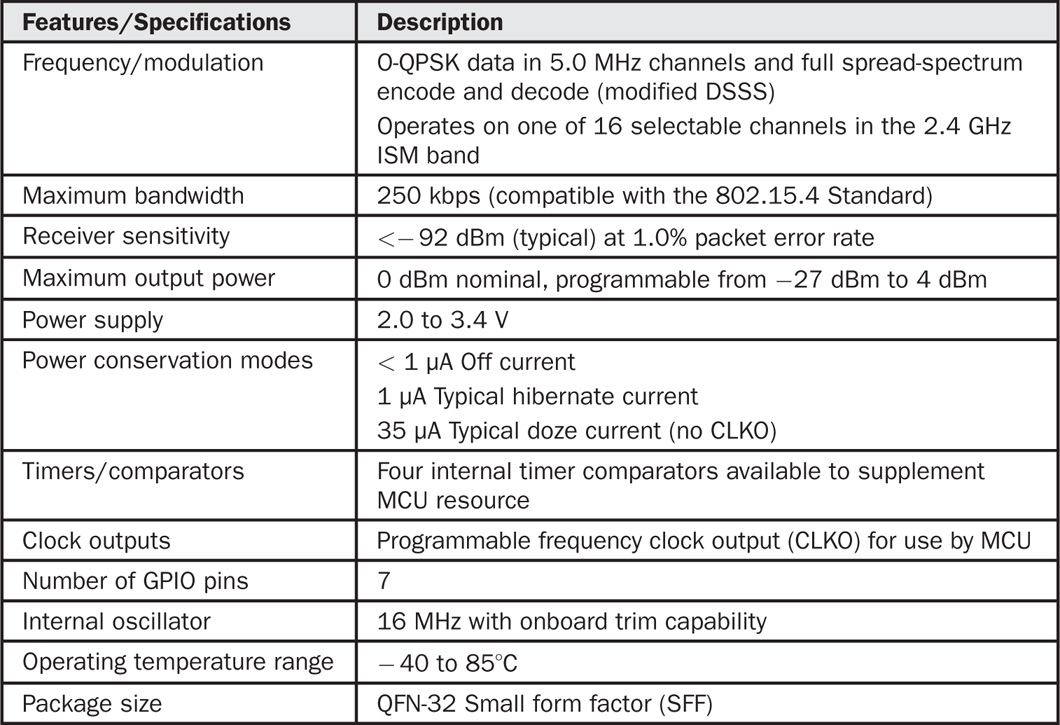
I selected the Parallax PMB-688 GPS receiver, which is small, lightweight, and very suitable for use in this project. Figure 8.7 is a picture of this receiver. The PMB-688 GPS receiver will track up to 20 satellite channels, which provides for both fast acquisition and the continuous lock of NMEA data from the satellites. Table 8.1 lists key specifications and features for this receiver.
Several key specifications are worth discussing a bit more. An acquisition sensitivity of –148 dBm means that the receiver is extremely sensitive to picking up weak GPS signals. The –159 dBm tracking sensitivity means that the signal, once acquired, can lose up to 90% of its original strength, yet remain locked in by the receiver.
Having an NMEA 0183 output operating at 9600 baud means that the receiver generates standard GPS messages at a rate twice as fast as comparable receivers. The 30-second start-up time is excellent and due in part to the receiver’s extreme sensitivity.
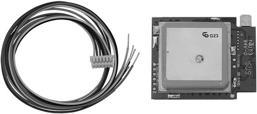
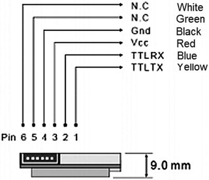
Universal Asynchronous Receiver Transmitter (UART) is the serial data protocol used between the GPS receiver and the Propeller Mini processor module (which is discussed in a later section). Three data pins are the minimal amount necessary to establish a communications link between the receiver and the processor. They are identified on the GPS as TTLTX (transmit), TTLRX (receive), and GND (ground or common), as shown in Figure 8.8.
The TTL in the pin designations represents the fact that the logic levels are 0 and 5 V for low and high levels respectively. The GPS receiver also uses a 9600-baud rate to communicate with the controlling microprocessor to both receive and transmit data back and forth. There is no need for a separate clock signal line, since the UART protocol is designed to be self-clocking.
CAUTION: To ensure communications with the Prop Mini module, connect the GPS TX lead to the Mini’s P8 pin, and likewise, connect the GPS RX lead to the Mini’s P9 pin. Misconnecting these pins will likely not cause any damage, but you will not have data communications between the GPS receiver and the Propeller Mini module.
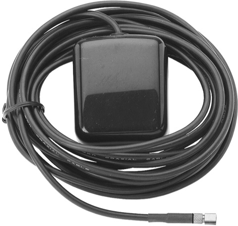
It would be wise to check that the PMB-688 GPS receiver is functioning as expected before going on to later stages in this project. Ensure that you have a good line of sight with the open sky to be able to receive the GPS satellite signals. I used an external GPS antenna because my test setup was indoors and had no reliable satellite reception. Parallax has an external GPS antenna available (part number 28502) that is shown in Figure 8.9 and is well worth the modest cost. Erratic or unreliable satellite reception will quickly cause this project to fail.
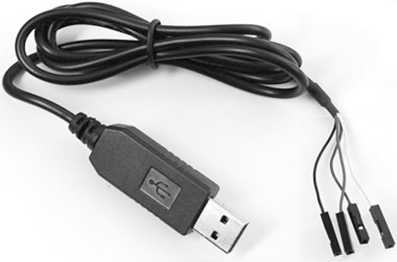
An interconnecting cable between the GPS and the monitoring laptop will also be needed along with a very useful Prolific USB-to-Serial software driver. The link is set up using a USB-to-TTL serial cable that is connected to the GPS receiver cable, as shown in Figure 8.10. This cable is available from Adafruit Industries as part number 954.
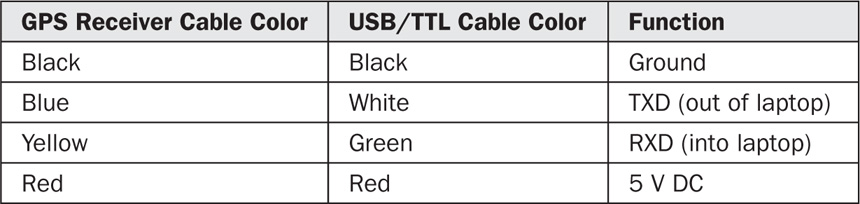
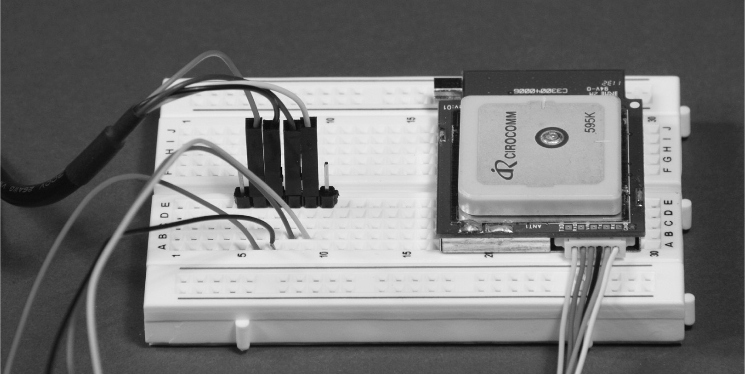
The USB/TTL cable has four pin connectors that are color coded and attached to the matching GPS receiver’s color-coded pin connectors, as detailed in Table 8.2. The physical solderless breadboard connections between the GPS receiver cable and the USB/TTL cable are shown in Figure 8.11.
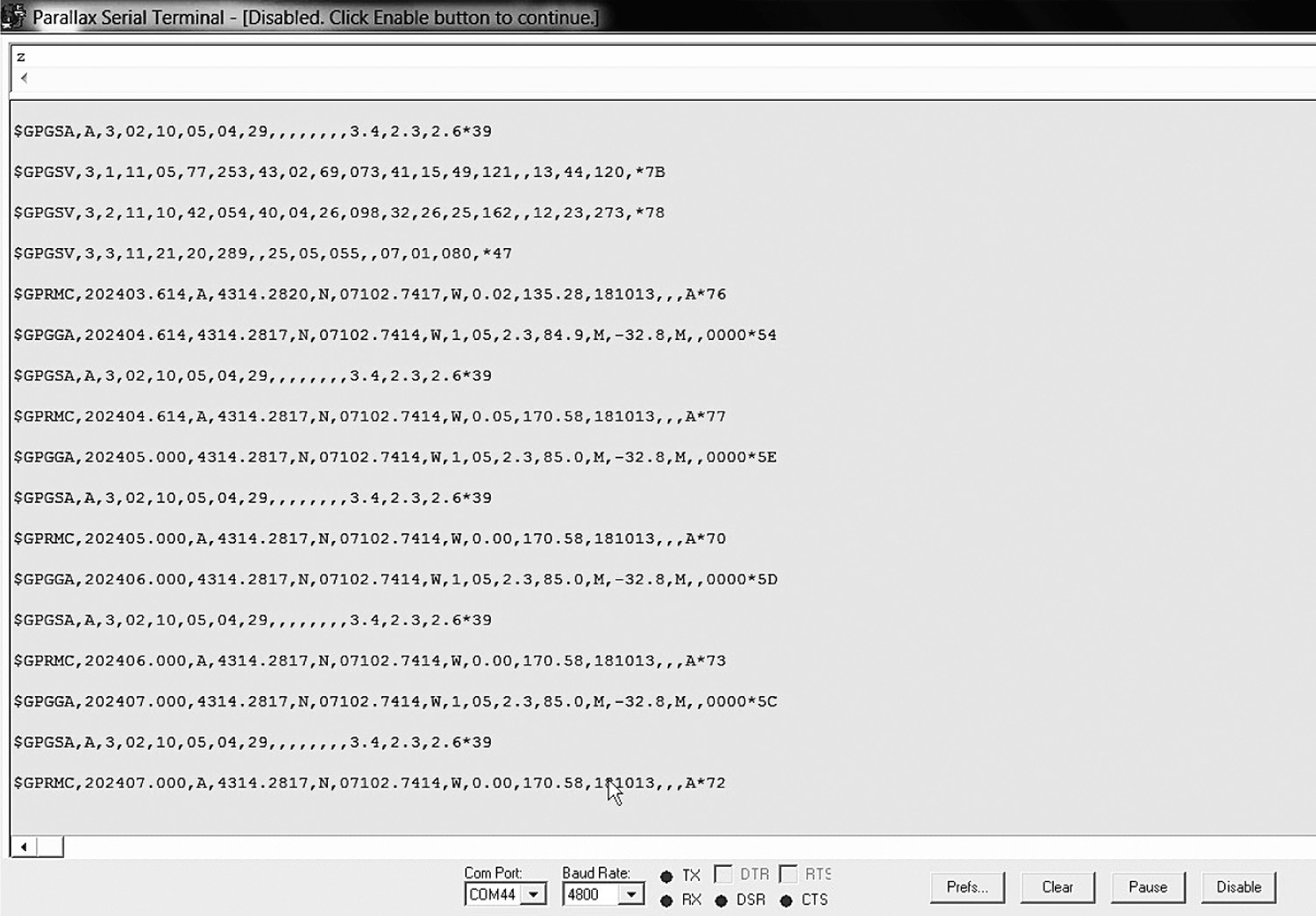
I used the Propeller Serial Terminal (PSerT) program with the baud rate set to 4800 to match the GPS receiver output. Additionally, COM port 44 was automatically assigned on the laptop by the Prolific software driver. Figure 8.12 is a screen capture of the GPS data stream showing that the GPS receiver was properly functioning and receiving good satellite signals.
Completing the above steps confirms that the PMB-688 GPS receiver is operating properly, which is a prerequisite before further project development. You are almost ready to start using the GPS receiver, but first I will discuss the NMEA protocol and the messages that are being generated from the PMB-688 GPS receiver.
As noted previously, NMEA is the acronym for the National Marine Electronics Association, but nobody refers to it by its formal name. NMEA is the originator and continuing sponsor of the NMEA 0183 standard that defines, among other things, the electrical and physical standards to be used in GPS receivers. This standard specifies a series of message types that receivers use to create messages that conform to the following rules, also known as the Application Layer Protocol Rules:
• The starting character in each message is the dollar sign.
• The next five characters are composed of the talker id (first two characters) and the message type (last three characters).
• All data fields that follow are delimited by commas.
• Unavailable data is designated by only the delimiting comma.
• The asterisk character immediately follows the last data field, but only if a checksum is applied.
• The checksum is a two-digit hexadecimal number that is calculated using a bitwise exclusive OR algorithm on all the data between the starting ‘$’ character and the ending ‘*’ character as well as including those characters.
There are a large variety of messages available in the NMEA standard; however, the following subset is applicable to the GPS environment and is shown in Table 8.3. All GPS messages start with the letters “GP.”
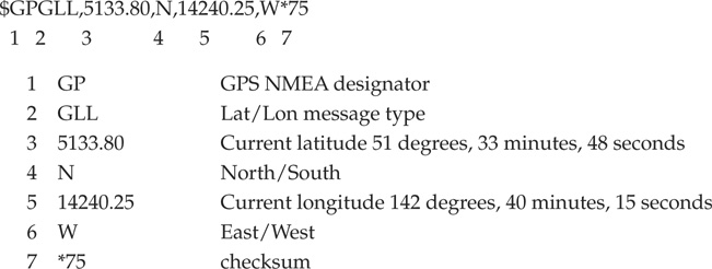
The two digits immediately to the left of the decimal point are whole minutes; those to the right are decimals of minutes. The remaining digits to the left of the whole minutes are whole degrees.
4224.50 is 42 degrees and 24.50 minutes, or 24 minutes, 30 seconds. The “.50” of a minute is exactly 30 seconds.
7045.80 is 70 degrees and 45.80 minutes, or 45 minutes, 48 seconds. The “.80” of a minute is exactly 48 seconds.
The following is an example of a parsed GPGLL message that illustrates how to analyze an actual data message:
All GPS applications use some type of parser application to analyze data messages and extract the required information to meet system requirements.
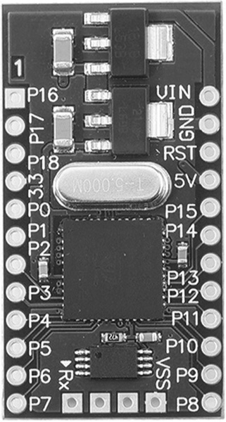
At this point I would like to take a moment to introduce you to the Propeller Mini module, which I used as the onboard processor for the GPS receiver. The Propeller Mini, which I will henceforth refer to as the Mini, is a relatively new Parallax module, just introduced in 2013. The module is very reasonable in cost and fully supports the full Propeller Spin programming language as well as any other Propeller-compatible language. Figure 8.13 is a picture of the Mini.
Key details and specifications for the Mini are shown in Table 8.4. I mounted the Mini on a solderless breadboard to gain easy access to all the general-purpose input/output (GPIO) pins. The breadboard will also allow for easy mounting and connections to both the GPS receiver and the XBee transceiver, which is discussed in the following section.
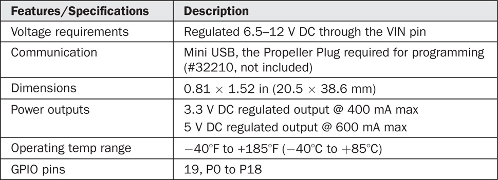
GPS data must be sent wirelessly from the quadcopter to a ground station where it is received and displayed for the operator’s use. I selected XBee transceivers to perform this function, since they are small, lightweight, inexpensive, and totally compatible with the other modules used in this project. XBee is the brand name for a series of digital RF transceivers manufactured by Digi International. Figure 8.14 shows one of the XBee Series 1 transceivers that I used.
There are two rows of 10 pins on each side of the module. These pins are spaced at 2 mm between each one, which is incompatible with the standard 0.1-in spacing used on solderless breadboards. This means that special connector sockets must be used with the XBee modules. Fortunately, Parallax has anticipated this issue and has provided several solutions.
I used two different approaches to mounting the XBee modules. The first was to use Parallax’s XBee SIP Adapter, which is shown in Figure 8.15 with an XBee mounted on it. SIP is an abbreviation for single inline package, which is a strange description if you look at the adapter’s bottom edge where two rows of pins are attached. The two-pin rows are just to provide mechanical stability, since the two pins in each row are electrically connected to one another.
The other mounting approach is actually part of the Parallax’s Propeller Board of Education (BOE) development board. The Parallax BOE designers thought that the XBee would be a very popular peripheral for this board, so they incorporated two 10-pin-row mounting sockets. The BOE is shown in Figure 8.16 with the XBee socket visible at the bottom center of the board. There is a microSD socket situated between the XBee sockets. The BOE designers also included eight socket pins where key XBee pins are easily available for interconnections. These pins are part of a 10 × 2 socket located above the right XBee socket.
I will next examine the XBee hardware to show how this clever design makes wireless transmission so easy.
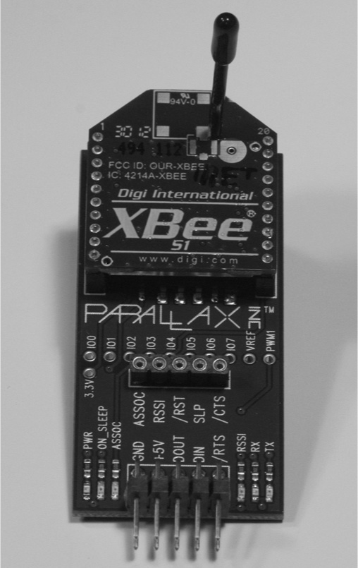
All the electronics in the XBee hardware, except for the antenna, are contained in a slim metal case located on the bottom side of the module, as may be seen in Figure 8.17. If you look closely at the figure, you should see the bottom of the antenna wire, which is located near the top left corner of the case. While Digi International is not too forthcoming regarding what makes up the electronic contents of the case, I did determine that the earlier versions of the Series 1 XBee transceivers used the Freescale™ model MC13192 RF transceiver. This chip is a hybrid type, meaning that it is made up of both analog and digital components. The analog components make up the RF transmit-and-receive circuits while the digital components implement all the other chip functions. It is a complex chip, which is the reason why the XBee module is so versatile and able to automatically perform a remarkable number of networking functions. Table 8.5 shows a select number of features and specifications for the MC13192.
The XBee module implements a full network protocol suite (which is discussed below in the software section), but from a hardware perspective, it means that there must also be a microprocessor present in the electronics case. From my research, I cannot determine which type of microprocessor it is, but I am willing to make an educated guess that it would be a Freescale™ chip, based upon the reasonable assumption that the MC13192 would be designed to be highly compatible with the company’s own line of microprocessors. One other factor supporting my guess is that Digi International has recently introduced a line of programmable XBee modules named XBee Pro SB that use the 8-bit Freescale™ S08 microprocessor. Of course, being able to put your own programs into the XBee would eliminate the need for the Mini, but that would not be as much fun and would probably be a bit limiting, given the tremendous capabilities of the Propeller chip.
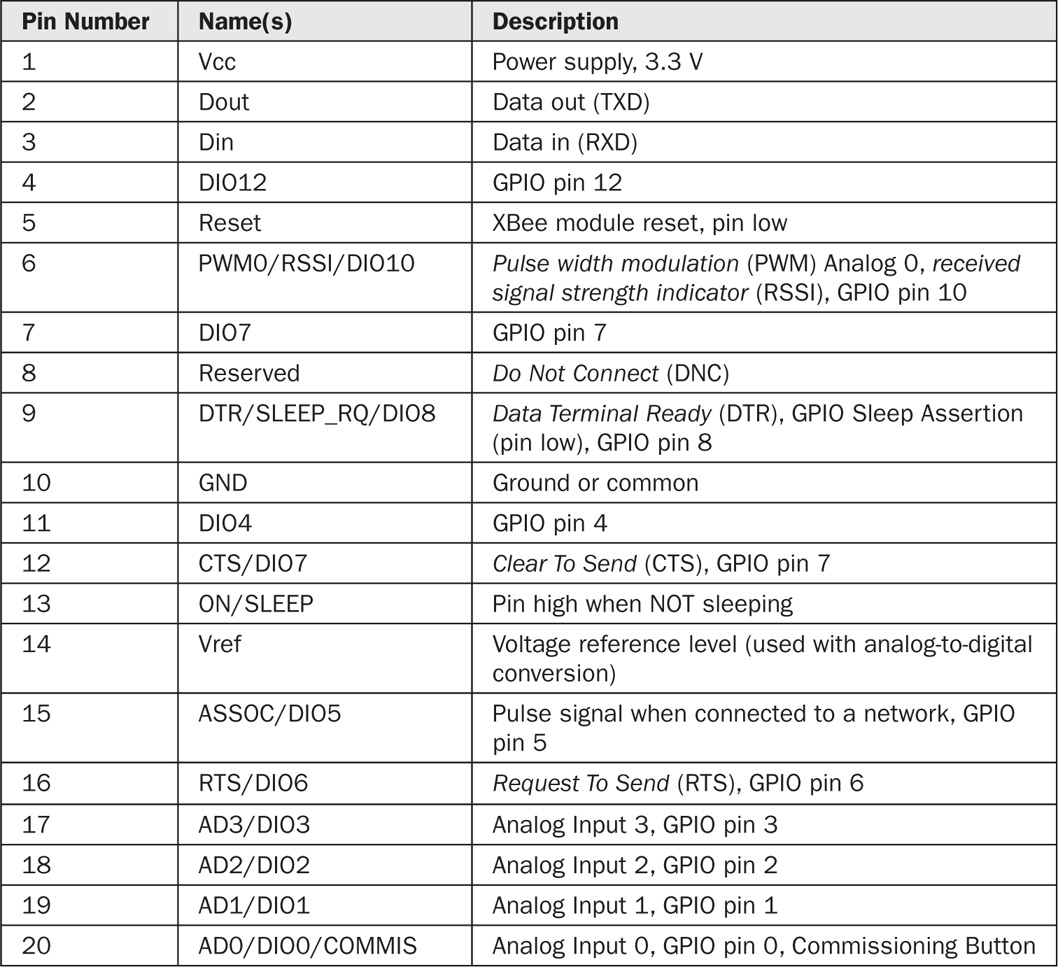
The XBee pins are detailed in a logical arrangement in Figure 8.18 for your information. Just be aware that only four of the pins are needed for this project, and they are shown with an asterisk next to the pin label. All the pin and function descriptions are shown in Table 8.6.
There are a considerable number of functions available to you if needed; however, this project requires only the most minimal functions for simple and reliable data transfers. Thankfully, the XBees automatically connect and establish reliable communications.
What is even more interesting than the hardware design is the data transmission and reception protocol that XBee implements, which I will discuss in the next section.
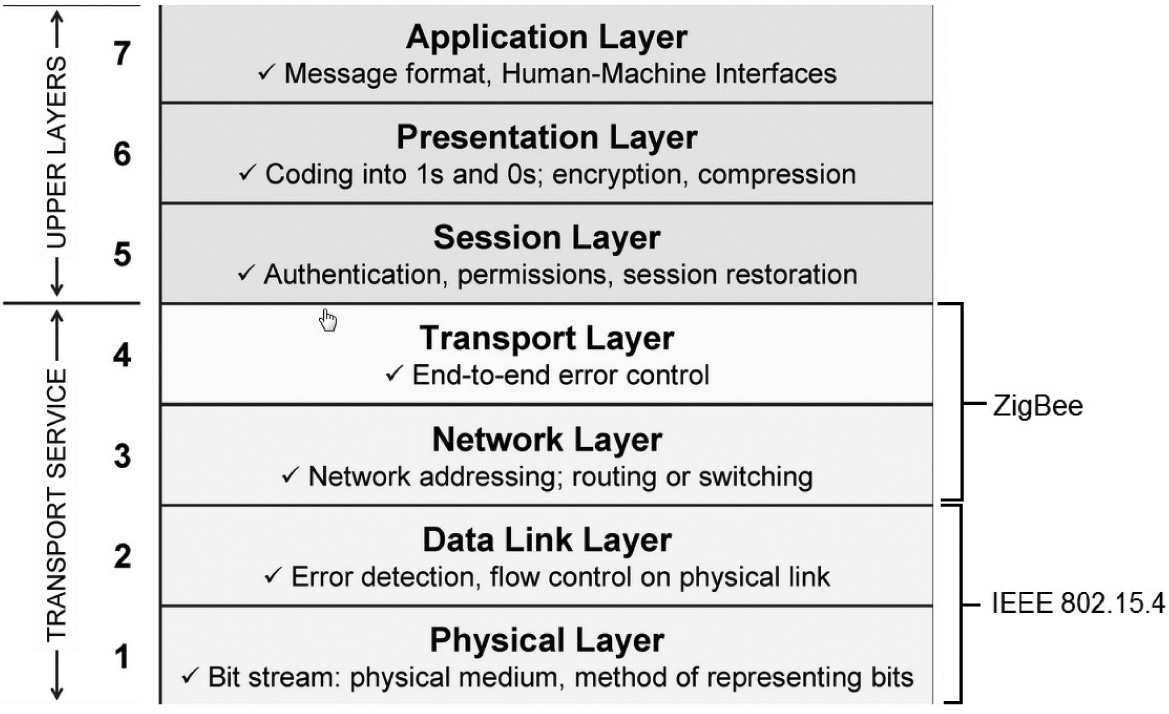
The XBee uses a highly capable networking protocol named ZigBee, which is also called a Personal Area Network (PAN). I will endeavor to keep the technical jargon to a minimum; however, it is important that you get at least a fundamental knowledge of how the ZigBee network functions in case something does not work as planned.
Zigbee was designed to be compliant with the ISO 7 Layer network model. As such, its inherent design is based upon proven computer network concepts that are robust, efficient, and well understood by most system designers. Figure 8.19 shows the ZigBee logical network stack with the corresponding ISO layer number. All subsequent network software developed for the ZigBee network follows this model.
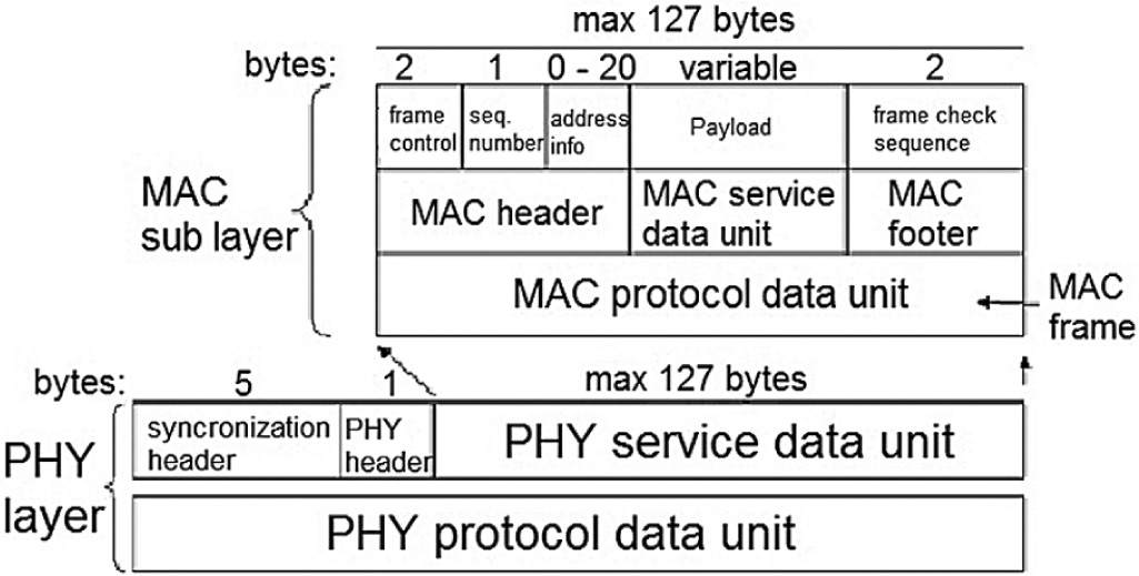
Data sent through the ZigBee network is in packets similar to the Ethernet format. Figure 8.20 shows how these packets are initially constituted at Layer 2, or MAC as it is referred to in the figure. These packets may be subsequently modified at higher layers, as needed, to suit the real-time network communication needs.
There are four packet types that exist in ZigBee:
1. Beacon
2. Data
3. MAC Command
4. ACK
Actual data packets are formed at the MAC, or layer 2, level where the data is prepended with both the source and destination addresses. A sequence number is also assigned to allow the receiver to determine the correct sequence of received packets. It is relatively easy to receive out-of-sequence packets in this type of network. Frame control bytes are also appended for error checking, which is the reason why ACK packets are required. ZigBee is a type of connection network, similar to Ethernet, that has a very robust way of ensuring that packets get where they need to go. ZigBee Layer 3 uses acknowledgement packet (ACK).
The receiver performs a 16-bit cyclic redundancy check (CRC) to verify that the packet was not corrupted during transmission. If a good CRC is determined, the receiver will then transmit an ACK; this action allows the transmitting XBee node to know that the data were received properly. The packet is discarded if the CRC indicates the packet was corrupted, and no ACK is transmitted. The network should be configured such that the transmitting node will resend up to a predetermined number of times until either the packet is successfully received or the resend limit is reached. The ZigBee protocol provides self-healing capabilities if the path between the transmitter and receiver has become unreliable or a complete network failure has happened. Alternate paths will be established if physically possible.
Layers 1 and 2 support the following standards:
• Star, mesh, and cluster tree topologies
• Beaconed networks
• GTS for low latency
• Multiple power-saving modes (idle, doze, hibernate)
Layers 3 and 4 further refine the packets by identifying what the packet type is, where it is going, and where it has been. They also set the data payload and support the following:
• Point-to-point and star network configurations
• Proprietary networks
Layer 4 sets up the routing, thus ensuring that the packets are sent along the correct paths to reach the desired nodes. This layer also ensures that:
• ZigBee 1.0 specifications are met
• Support is provided for star, mesh, and tree networks
There are also three ZigBee standards that primarily involve Layers 3 and 4. These standards are:
1. Routing—Defines how messages are sent through ZigBee nodes. Also referred to as digi-peating.
2. Ad hoc network—Creates a network automatically without any operator involvement.
3. Self-healing mesh—Determines automatically if a malfunctioning node exists and reroutes messages, if physically possible.
Layer 5 is responsible for security, which is enforced by using the Advanced Encryption Standard (AES) 128-bit security key.
It is now time to demonstrate how the XBee works by using a simple test configuration between two XBee nodes and the Propeller boards controlling these nodes. Figure 8.21 shows the test configuration in which the XBee transmitter is being controlled by the Mini, and the XBee receiver is being controlled by the BOE.
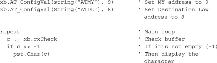
Two separate programs need to be loaded into each of the Propeller boards, one for transmit and the other for receive. The transmit program is named Test XBee Transmit.spin, and the source code is shown below:

This program and the following program were downloaded from the Parallax OBEX forum. Both programs were very slightly modified for this project. Note that the transmit program uses a BOE object named Propeller Board of Education and referenced as system, which also works perfectly with the Mini board. I am constantly impressed with how well Propeller software objects function among different development environments. It is a testament to the simplicity and consistent architecture used in the Parallax programming languages.
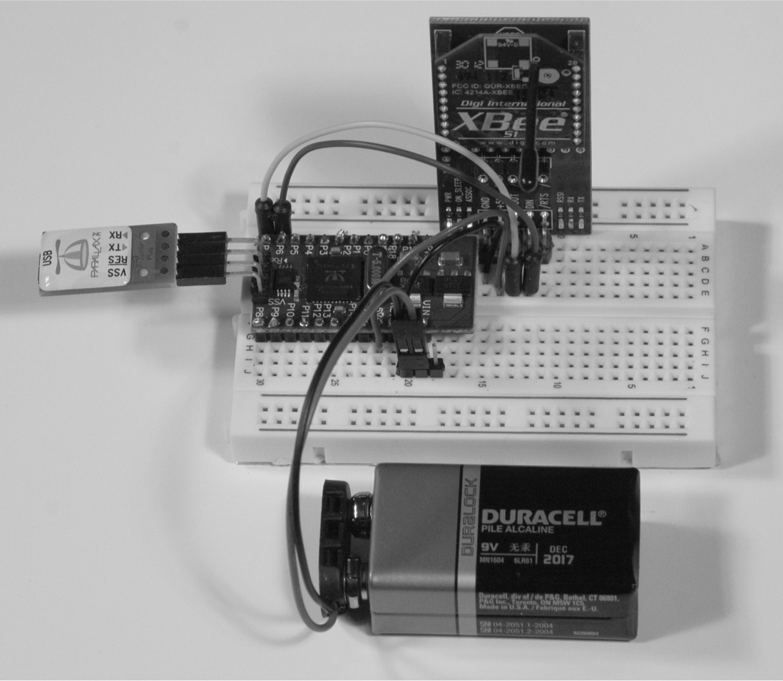
Figure 8.22 is a photo of the XBee mounted on an SIP adapter that is connected to the Mini—all mounted on a solderless breadboard. The whole transmitter assembly is powered by a single 9-V battery, which is also shown in the photo.
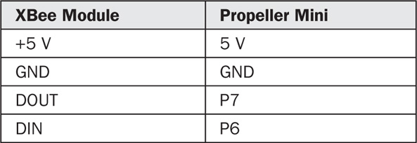
The Propeller Plug programming tool is also shown attached to the Mini in the figure. It is needed only to program the Mini for this project. There are four connections needed between the Mini and the XBee module, which are shown in Table 8.7. Of course, the Mini must be powered, which in this case, is with a 9-V battery connected to VIN and GND. Be sure you watch the polarity connection.
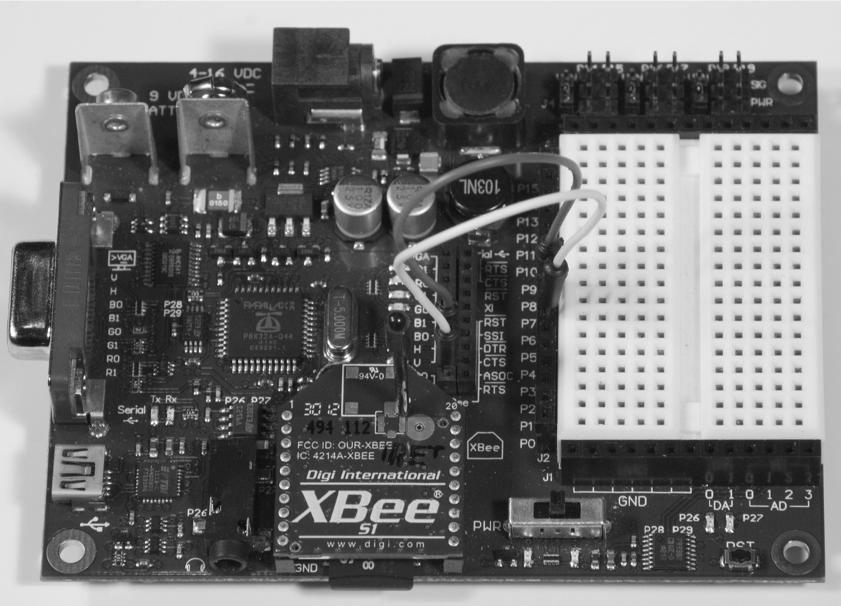
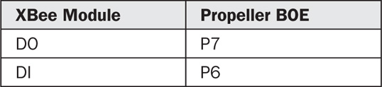
The transmit program will continuously send the phrase, This is a test, two times per second. The complimentary receiver node is composed of an XBee mounted on a BOE. This assembly is shown in Figure 8.23. Only two connections are needed between the BOE and the XBee module, as shown in Table 8.8. The BOE is powered through the mini USB cable that attaches to the laptop running the PSerT program, while the XBee module is powered through the BOE sockets.
The receive program is named Test XBee Receive.spin, and the source code is shown below:
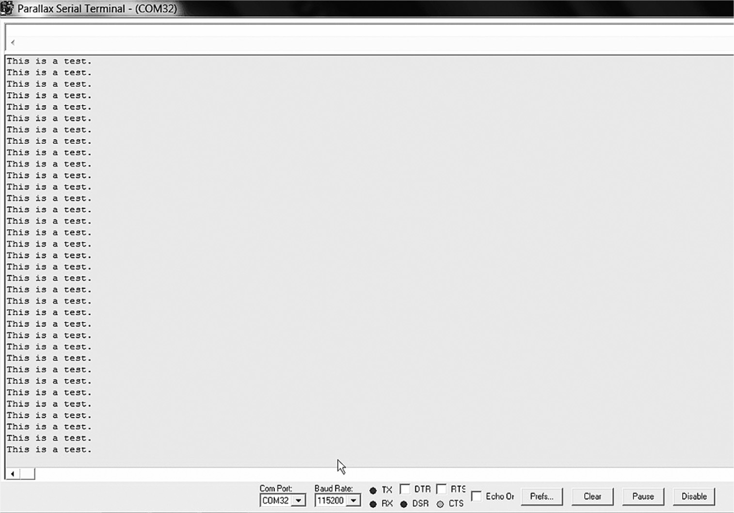
The receive program uses the same objects as the transmit program with the addition of the Parallax Serial Terminal Plus object, which enables the display of the received data on the laptop screen that is running the PSerT program. Figure 8.24 is a screenshot of the laptop screen that is running the PSerT application for the data transmission test.
I performed a simple range check to determine the approximate operating range for the XBee test system. The transmitter node was set on a tripod at one end of a large, open field. I then walked away from the transmitter while carrying a laptop running the test program. I walked approximately 114 paces from the transmitter, at which point the transmission became intermittent. My pace is about one meter, so that was a good estimate for the reliable range. I walked a bit further and continually repositioned the receiver node to see if the signal could be reacquired. I was able to go out to about 154 m, at which point no amount of node juggling could get the signal back. The 114-m distance is actually a bit better than the stated 100-m range in the Zigbee specification.
Digi International also manufactures a line they call the XBee Pro, which generates up to 60 mW of power—much greater than the regular Series 1 power output of 1 mW. The Pro brochure claims a line-of-sight range of up to one mile. That is an impressive range, but I am fairly sure that it would far exceed the range of the R/C transmitter and the FPV camera system, which will be discussed in the next chapter. In any case, I believe that the quadcopter would be invisible to the operator at such a distance, which is never a good idea.
The range check confirmed that the XBee modules appropriately support operations at or below 300 feet when they are above ground and reasonably close to the operator’s control station.
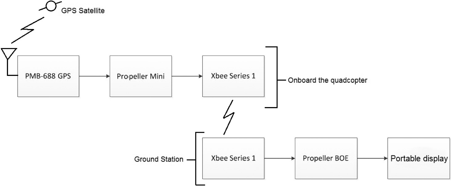
A block diagram of the complete GPS system is shown in Figure 8.25.
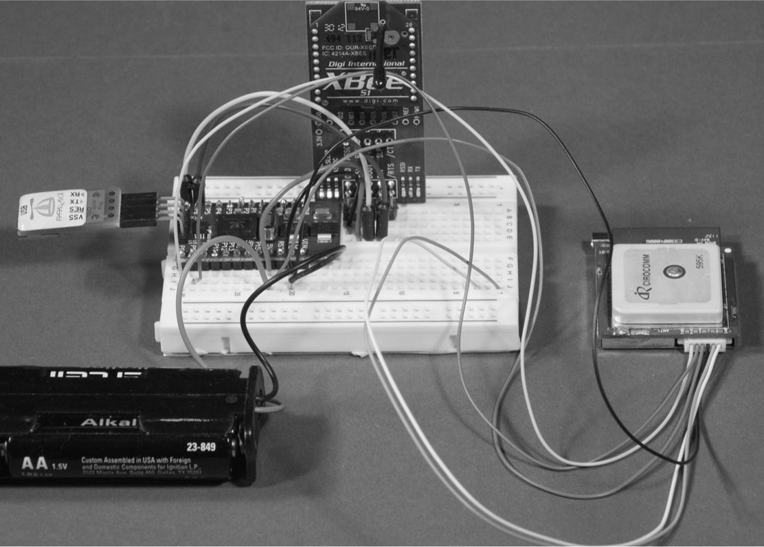
In the complete system, unlike the test system, the PMB-688 GPS module is connected to the Mini as the data source, and a portable display is used in lieu of a laptop for the receiver node. Figure 8.26 shows the prototype assembly for the transmitter node as it was set up for testing.
You should note that I changed the power source from a 9-V battery to a six pack of AA cells. The additional current draw of the added GPS module quickly drained the 9-V battery, while the battery pack capacity was much higher.
All GPS and Mini interconnections are shown in Table 8.9. All of the interconnections between the XBee and Mini are still in place and remain as they were detailed in Table 8.7.
Note that the GPS yellow wire is named TTLTX, which means that data are output via this wire. This yellow wire is actually the receive line, which can be a bit confusing. Just remember that data-communication port nomenclature is usually specified from the perspective of the module, that is, data coming out of the module is TX, while data going into the module is RX.
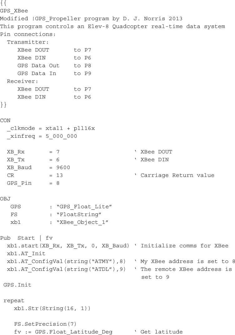
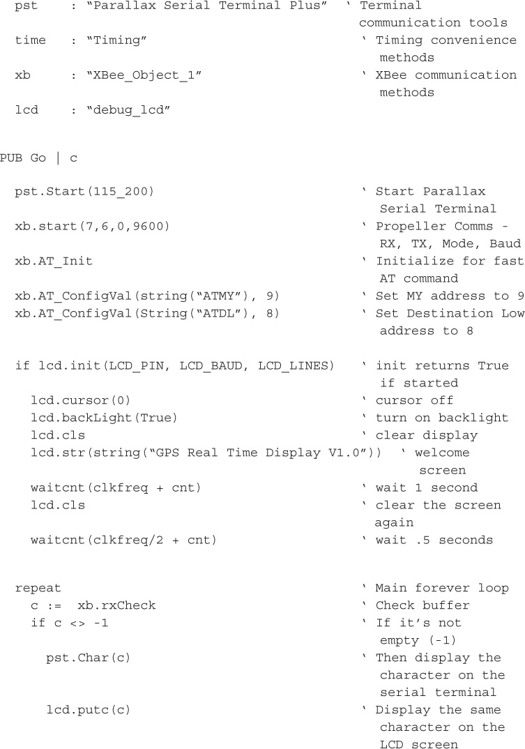
The program that is run in the Mini is significantly different from the test program shown above. It now incorporates a GPS driver object as well as the existing XBee object. It also contains a considerable amount of code to parse, or separate, the raw NMEA data that is streaming from the GPS PMB-688 module. The Spin object is named GPS_Propeller, and the code is shown below.
The above program uses the same XBee driver object, XBee_Object_1, as was the case in the previous test programs. This program also uses a GPS driver object named GPS_Float_Lite that takes care of all the necessary protocols between the GPS module and the Mini. Retrieving data from the GPS module becomes very easy, since all that is required is to call the GPS driver method that returns the desired data. For example, the following gets the current GPS hour data:
fv := GPS.Long_Hour
Where fv is a local variable, GPS is the local reference to GPS_Float_Lite, and Long_Hour is the name of the method in GPS_Float_Lite that returns the current GPS UTC hour value. UTC is short for Coordinated Universal Time and is the time standard used to ensure that GPS time reports become independent of any time zone.
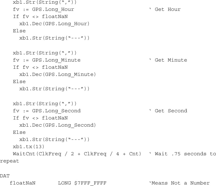
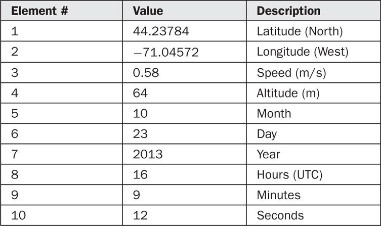
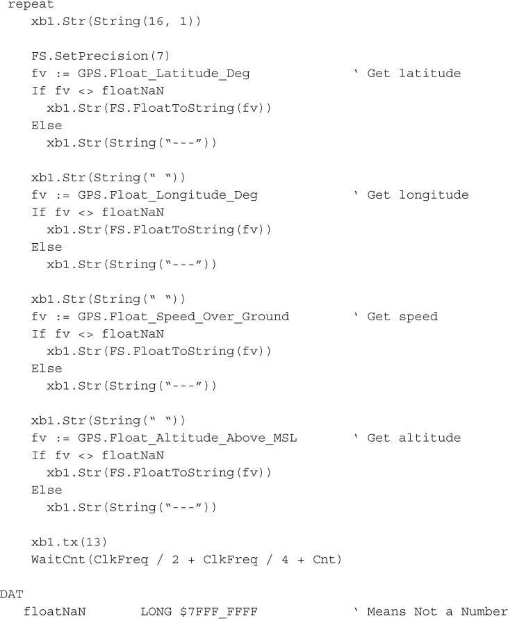
Except for the deployed display, the receive portion of this system is the same as the one previously described in the test system. I used the BOE with the laptop to test the prototype system, which made sense because the portable display would not impact any essential data transfers between the transmitter and receiver XBee nodes. The receiver-node connections were detailed in Table 8.8, and the assembly was shown in Figure 8.23. Figure 8.27 is a laptop screenshot showing the results of a trial run with the complete GPS system. The 10 data elements displayed in the figure are detailed in Table 8.10 for your information. GPS data is updated every 0.75 seconds, which allows sufficient time for the GPS module to receive a fresh data set. Please note that the GPS module provides the coordinates in decimal degrees with the minutes and seconds as a decimal fraction of a degree in lieu of the NMEA format discussed earlier. It is fairly easy to make the conversion to integer minutes and seconds using software, if that is the required format.
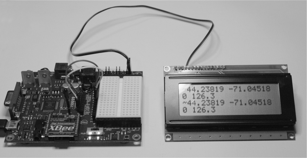
I used a 4 × 20 LCD for the portable display because I wanted to show only latitude, longitude, speed, and altitude. It really is not very critical to display the date and time for real-time quadcopter control. I used the same LCD display that I described in Chapter 7 for the servo-signal pulse-width display. I also slightly modified the code to display the four GPS data elements instead of the pulse widths. Inserting the LCD display code was also quite easy, since I only had to add the LCD display-driver object and reference the input data pin, which is P19. Incidentally, I also left the PSerT driver code in place, since I figured it might come in handy for any debugging.
Figure 8.28 shows the LCD display with the four GPS data elements. They are repeated twice because of the simple character-by-character transmission scheme that is being used. I do not consider this side effect to be much of an issue.
The modified Test XBee Receive program is shown below.

I chose to connect the LCD display to pin 19 because that is also a BOE servo port. That way, I could use a servo cable to connect the LCD display with the BOE as I did in Chapter 7.
The transmit code was modified to transmit only the four GPS data elements discussed above. I also eliminated the commas between the data elements to conserve space on the LCD display. The modified transmit program named GPS_XBee_Brief is shown below.
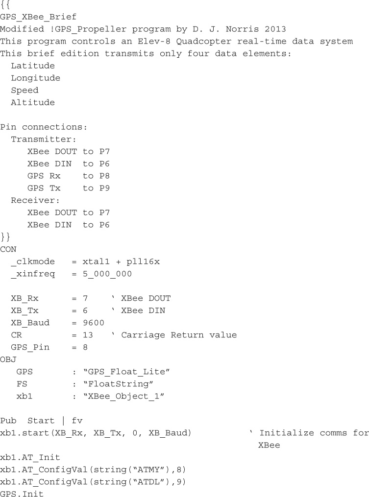
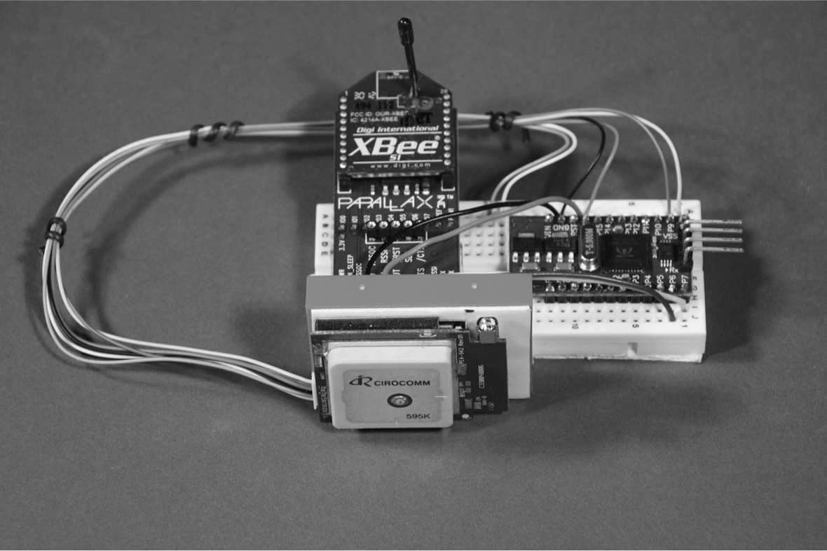
Figure 8.29 shows the front of the XBee transmitter node assembly. I wanted to use the XBee SIP-mounting adapter but did not want to mount it vertically in a solderless breadboard. I was concerned about the quadcopter vibrations shaking loose the somewhat top-heavy XBee assembly. After a bit of thought, I came up with the configuration that you see in the figure, where the SIP assembly is still plugged into a breadboard. However, the breadboard itself is attached by foam-backed, double-sided tape to another breadboard that holds the Mini. I also put a hidden spacer between the SIP adapter and the horizontal breadboard to increase the overall rigidity of the assembly. The GPS module is mounted to the back of the vertical breadboard, as you can see in Figure 8.30.
The GPS is held in place by the double-sided tape that is normally attached to the bottom of new breadboards. You should be aware that a vertically mounted GPS module with an internal antenna is not as sensitive to satellite signals as a horizontally mounted one is. You might want to initially hold the quadcopter on its side with the flat side of the GPS antenna pointed to the sky until a signal is acquired. Once the receiver locks on to the satellite signal, the red LED will be steady instead of blinking. The receiver’s hold sensitivity is much better than the acquisition sensitivity, so the quadcopter can be put back to a horizontal position while still locked onto the GPS signals.
NOTE: The original intent of this section was to demonstrate how to display the quadcopter’s position in real time by using the Google Earth application. Unfortunately, I was never able to stream the raw GPS data successfully from the XBee transmitter to the ground-station XBee receiver, and then into a laptop running Google Earth. However, I do show you how to manually enter the coordinates as they are displayed on the LCD screen so that you can have a near real-time location service.
I selected the Google Earth application for the moving map display because it incorporates a very convenient interface that accepts serial GPS coordinates and can display them on a computer screen in real time. This project was divided into several phases so that I could experiment with the various technologies involved with the moving map and determine how to best implement each phase. The first phase was simply to use an existing hand-held GPS device plugged into a laptop running the Google Earth application.
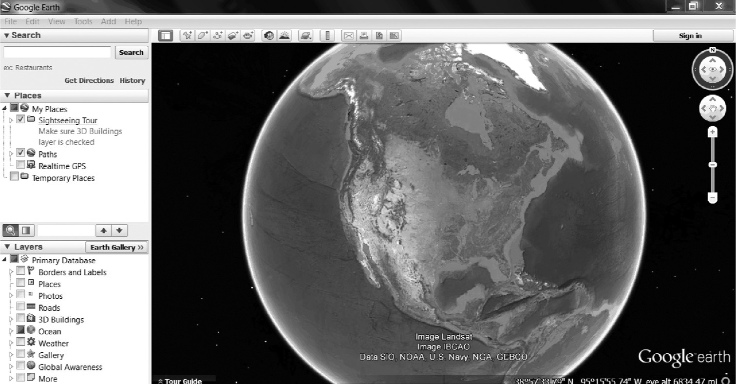
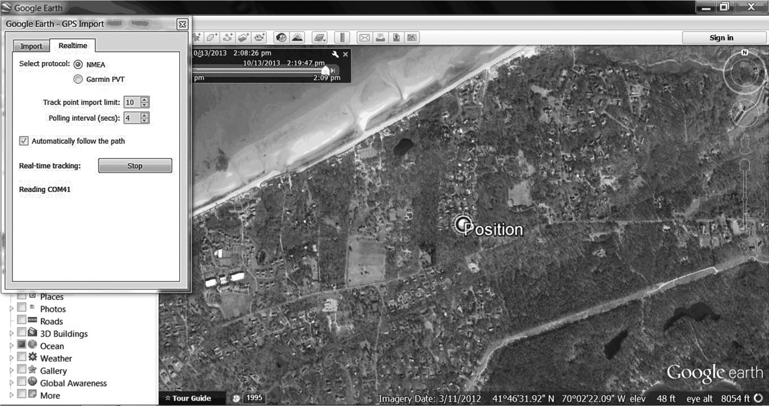
Figure 8.31 shows the Google Earth opening screen. I ran the application on a Win7, 11.3-in, and 32-bit Toshiba laptop. You next have to click on the Tools menu bar selection to access the GPS import function. Figure 8.32 shows the real-time GPS menu selection.
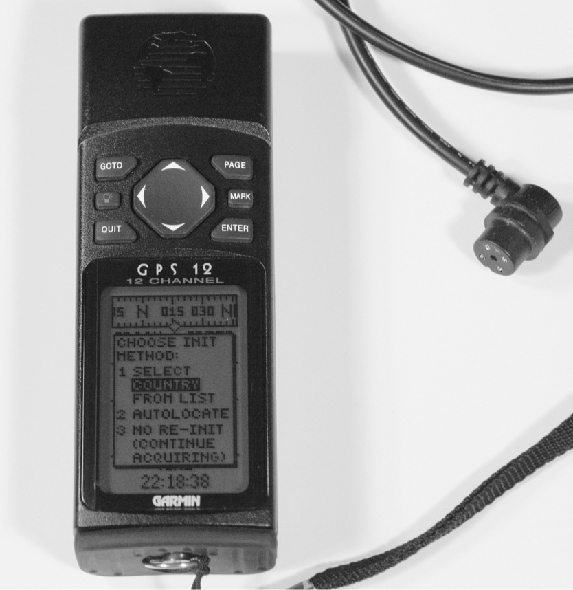
Ensure that the NMEA box is checked because it is the data format used by the majority of GPS receivers. Google Earth also has a very nice feature that scans all the available serial ports in order to identify the active one with the serial GPS data. You can observe this behavior simply by plugging a GPS receiver into a computer’s USB port. I used an older style GPS receiver that is shown in Figure 8.33 to provide the GPS data stream.
You can also see in the figure a portion of the older-style RS-232 cable that plugs into the back of the receiver. This type of cable requires an RS-232-to-USB converter to make it compatible with a modern USB port. I used one of the ubiquitous converters commonly available at local office supply stores to adapt my old-style cable.
Figure 8.34 shows the results of a real-time import using the GPS12 receiver plugged into the laptop. The bulls-eye Position indicator shown in the figure was automatically added by the application. Also, the 8000-ft altitude for the view seems to have been automatically selected by the Google Earth program. I tried to lower it, but it reverted to the higher altitude, as shown in the figure. I don’t believe this view altitude will be too much of an issue because the 8000-ft, above-ground altitude is a good compromise between detail and overall area coverage. In addition, the 4-second polling interval is a reasonable number, since the Elev-8 should not travel too far in a 4-second period.
Entering coordinate data into Google Earth is very easy. Simply type the coordinates into the Search text box, and press the Enter key or click on the Search button. For example, I entered the following coordinates, using the decimal-degree format, into the Search text box:
42.23978 N 71.04598 W
Ensure that there is one space between each element and that descriptors N and W are also present. Of course, the N and W descriptors will change depending upon where you operate the quadcopter. Figure 8.35 shows the resultant Google Earth screen when the above coordinates were entered into the Search text box.
This section completes my discussion of how to achieve good situational awareness when operating the quadcopter while using a real-time GPS system. The next chapter shows you how to add real-time video capability that will greatly complement this GPS system.
I began the chapter with a brief history of the GPS system followed by a tutorial that used a fictitious example to explain the basic underlying principles governing the system.
The PMB-688 GPS receiver was discussed next, focusing on its excellent receiver characteristics as well as its easy serial communication link.
I discussed how to set up and test the GPS module with a serial-console link by using a USB/TTL cable. The Propeller Serial Terminal (PSerT) was run on a Windows laptop to verify proper operation of the GPS module.
The NMEA 0183 protocol was thoroughly examined to illustrate the rich set of messages that are created by the GPS receiver. This project uses only a small subset of the data, but you should be aware of what is available for potential use. A look at a parsed GPS message was also included along with a brief explanation of how to interpret latitude and longitude data.
The next item introduced was the new Propeller Mini, which is a very compact Parallax Propeller development module. This module supports the full Spin language with a full complement of general-purpose input/output (GPIO) pins. I used the Mini as an onboard controller for both the GPS module and an XBee RF transceiver.
I also carefully explained Zigbee, which is the XBee data communication protocol. It is important to understand how Zigbee works because it is a key part of the control program that runs in the controlling microcontroller.
The XBee functional test demonstrated how simple it is to set up a communications link that could transfer GPS data. The operational software for both the transmitter and receiver nodes was described, and I determined the operational range for the XBee link, which is compatible with the Elev-8 operating profile.
Next, we looked at a complete GPS system and the modified software for the transmitter node. I showed how the system displays GPS data on a PSerT screen and on a portable LCD display. The latter display makes it easy to use in a field-deployable ground station.
I showed a compact design for an onboard GPS/XBee module that may be easily mounted on an Elev-8. The design is resistant to disruptions that might be caused by quadcopter vibrations.
The chapter concluded with a look at how to use the Google Earth application with real-time GPS. I explained how easy it is to enter GPS coordinates manually into Google Earth to show the quadcopter’s position in the application.