Figure 1. Was this sequence flipped or faked?
Probability is a beautiful and widely applicable branch of mathematics. Here we present a few of the basic concepts of probability as an application of set theory, functions, and other topics from the first several chapters. Probability functions, random variables, and expected value are introduced, motivated by the question of how you might guess if a sequence of coin flips is real or fake. Have some dice, coins, and cards on hand: many of our examples and exercises involve these and related games of chance.
One morning, Professor P passed out the following two-page homework assignment to a class of 40 students:
Page 1: Flip a coin once. Write down H or T for the result:
Page 2: If your result on Page 1 is H, flip that coin another 250 times, and record the sequence of results in the blanks below.
If your result on Page 1 is T instead, don’t flip the coin again. Instead, make up a sequence of Ts and Hs that you believe is a reasonable simulation of flipping a coin 250 times in a row, and record that sequence in the blanks below.
, , , , , , , , , , , , , , , ,
, , , , , , , , , , , , , , , ,
, , , , …
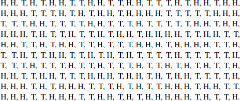
At the next class meeting, Professor P told each student to keep Page 1 as a receipt and turn in Page 2. She then scanned the responses on Page 2 carefully and quickly, taking no more than 30 seconds to declare each submission either “flipped” or “faked.” She wasn’t always correct, but her success rate was quite high, greater than 80%. How is this possible? One of the submissions is presented in Figure 1. Can you tell if it was flipped or faked?
We will discuss her method of analysis later in this chapter, but for the moment let’s informally introduce a few concepts that might assist with an initial approach. We will assume that the coin is fair, meaning that, on any single flip, it has the same likelihood of showing H or T. We will also assume that successive coin flips are independent, so that one flip doesn’t have any bearing on another flip. These two assumptions imply, for example, that if you are about to flip a coin twice in succession, each of the 2-flip strings HH, HT, TH, and TT is equally likely to occur.
Exercise 9.1 If you are about to flip a coin three times in succession, how likely are you to get exactly two Hs among the three flips?
Exercise 9.2 If you are about to flip a coin four times in succession, how likely are you to get no more than two Hs among the four flips?
These ideas suggest an approach to analyzing the students’ submissions. First, count the occurrences of Hs and Ts and see if they are roughly the same. Also, count the occurrences of the 2-flip strings and see if all four counts are roughly the same. Here, a question arises: should we only count the 2-flip strings that start in odd-numbered positions, to avoid issues of overlap? For example, if the first and second flips result in the 2-flip string HT, the second and third flips can only give TH or TT.
Exercise 9.3 Perform the counts just mentioned on the example in Figure 1. Do they provide evidence that the student actually flipped the coin? Or do you think the student faked the sequence of heads and tails?
After Professor P made all of her guesses and surprised the class with her accuracy, she noted that 32 of the 40 students had faked their flips. Given that a single fair coin flip determines which students should have faked their answers, it is reasonable to assume that approximately half the sequences would have been fake. How likely is it that as many as 32 were faked?
She playfully admonished the students as they left class that day. Although she couldn’t point a finger at any particular student, she knew with great confidence that at least a handful of students had not followed the rules of the assignment.
In this chapter we explore randomness and some of the basic ideas and examples of the mathematical theory of probability. We begin by introducing common terms used in probability theory that merely rename concepts from Chapter 3.
DEFINITION 9.1. A sample space is a set S. A sample point is an element of S. An event is a subset of S.
In applications of probability, we usually think of these terms in the context of an experiment or study where the possible individual outcomes are the sample points and the set of all sample points is the sample space. For example, when flipping a coin twice in a row, the sample space is the 4-element set {HH, HT, TH, TT}, and the event described by “get at least one head” is the subset {HH, HT, TH} containing three sample points.
In our 2-flip example, the sample space is  . If we are considering the case of a fair coin and independent flips, then the probability
  assigned to each sample point should be the same:
![]()
But notice that our definition of a probability function is quite general and allows us to consider distributions of probability values that don’t necessarily correspond to physical objects or prior experience. For example, defining  by
by
![]()
is totally fine from an abstract viewpoint because the individual probability values are non-negative and sum to 1.
Thus, the event X = “get at least one head” has probability  using
using  because
![]()
while using the probability is
![]()
A probability function gives a uniform distribution when  for all
  , and thus
 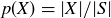 for any event
  .
.
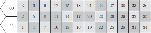
EXAMPLE 9.4. In the game of American roulette, a ball comes to rest in one of 38 positions on a spinning wheel labelled
![]()
The cells 0 and 00 are usually green and give the casino the edge when players make bets on the outcome of a spin. Half of the other 36 cells are red and half of them are black. For a single spin of the wheel, the sample space S is the set containing all 38 of the labels listed above, and the gambler’s assumption is that the probability distribution is uniform: the probability of landing in any particular cell is  . The event “lands on green” is
  , and the event “lands on red” is a subset
  with
with  . Thus,
  and
and  .
.
Exercise 9.4 A European roulette wheel is similar, only it has no cell labeled 00. What are  and
and  in European roulette? Is a ball more likely to land on a red position on an American wheel or on a European wheel?
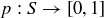
EXAMPLE 9.5. Roll two dice, one black and one white. Proposition 2.13 tells you that there are  possible outcomes; the chart in Figure 2 has the outcomes grouped in columns by their sum, with the black roll in bold. The sample space S contains all of these ordered pairs, and under the assumption that the dice are fair and the rolls are independent, the probability distribution is uniform. The event “the sum is nine” is
  , and the event “the sum is less than seven” is a subset
  with
with  . Thus, the probabilities of the events are
  and
and  .
.
We will refer to rolling a pair of dice several times in later sections of this chapter.
Exercise 9.5 Let E correspond to the event “the sum of two dice rolls is even,” and let T correspond to “the sum of two dice rolls is 3, 7, or 11.” What are  and
and  ?
?
Exercise 9.6 You are playing Monopoly, and in order to avoid landing on someone’s property you need your roll of two dice to sum to a value other than 5, 6, or 8. What is the probability you will succeed?
EXAMPLE 9.6. There are many situations where probability functions are defined for infinite sample spaces, and here we present just one example. You decide to flip a fair coin until heads comes up for the first time. The process will most likely terminate after no more than a few flips, but there is no guarantee that it won’t continue indefinitely. Thus, an appropriate sample space is the infinite set
![]()
Let  be the length of a flip sequence s. Our previous discussions of coin flips tells us that we should define
  for each
  , so
, so
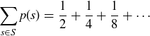
Quoting the geometric series formula from Section 8.4, this series converges to the value 1, so p is a probability function on S. The event  “the process ends by the third flip” is
  , which has probability
![]()
Exercise 9.7 Get together with some friends and flip a coin until it lands heads up for the first time.1Repeat this activity at least 40 times, keeping a list how many flips were required. What proportion of the sequences are at least four flips in length?
We conclude this section by discussing just a few of the many ways that probability functions behave with respect to set-theoretic operations on events.
PROPOSITION 9.7. Let A and B be events in a finite sample space S, with a probability function 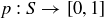 .
.
(a) If  , then
![]()
(b) If  is the complement of A in S, then
![]()
(c) The probability of the union is given by
![]()
PROOF. In each case we simply need to use the fact that
![]()
To establish (a), notice that when  ,
,
![]()
which is non-negative because  for all .
Since  , we have
![]()
which proves (b).
Finally, if  then
then  is a term in both the sum for
  and the sum for
  . Thus when
  the probability is double-counted in the sum
  . So
. So

You may have used an argument similar to the one just given for part (c) when you established the formula for  in your proof for Exercise 3.18(a). We note that when A and B are mutually exclusive events, meaning A and B are disjoint sets, then the probability of their union is simply
![]()
Proposition 9.7 holds for any probability function on S. Unless we state otherwise, for the rest of the chapter and exercises we will only consider probability distributions that are uniform, so the primary task is computing the sizes of sample spaces and events. To do this we often use Propostion 2.13, especially when each sample point corresponds to a sequence of outcomes like coin flips, and we also need combinations.
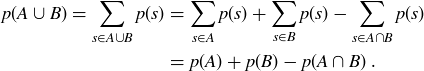
The enumeration ideas from Section 3.8 – where we introduced  – make it easy to determine the probability of an event such as having a sequence of five coin flips contain exactly three heads. The values of
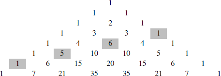
  , which count k-combinations of an n-element set, are often presented in the form of Pascal’s Triangle, as shown in Figure 3. There are many remarkable patterns in Pascal’s Triangle, several of which are the focus of end-of-chapter exercises. The most important relationship occurs between two consecutive entries in a row and the entry below them.
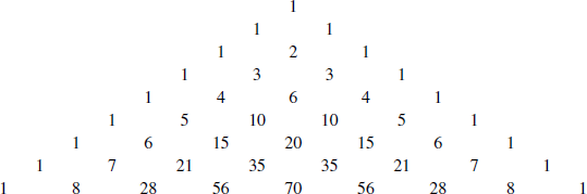
Figure 3. The first nine rows of Pascal’s Triangle. If the numbering of both the rows and the entries within a row begin with 0, then the ith entry in row j is  . For example, the left-most 15 you see is
  .
.
PROOF. Let S be an  -element set, and let a be any element of S. There are
  subsets of S with
  elements, and any such subset X is in exactly one of the following two cases:
(1)  ,
,
(2)  .
.
There are exactly different X that fall in case (1), because X contains a along with k of the remaining n elements in S. And there are exactly  different X in case (2), because X contains
  of the n elements in
  . The formula follows from summing these two quantities together.
Theorem 9.8 allows you to quickly generate the top rows of Pascal’s triangle: after plotting the 1s on the left and right borders, every other entry is the sum of the two entries on either side of it in the previous row. For example, the first 28 in the bottom row of Figure 3 is the sum of the 7 and 21 that sit above it.
Exercise 9.8 You may notice that each row of Pascal’s Triangle is both “symmetric” (it’s the same reading from the left or from the right) and “unimodal” (the terms increase toward the middle and then decrease). Prove both of these properties using the factorial formula given in Theorem 3.18.
At the beginning of this section we posed the question: What is the probability that a sequence of five coin flips contains exactly three heads? The sample space consists of all sequences of heads and tails of length 5, for a total of  sample points, so the probability of any given sequence is
  . We can count the number of sample points in our event using a one-to-one correspondence between the sequences with exactly three heads and the 3-element subsets of
  . The chosen elements correspond to the locations of the heads; for example,
  corresponds to HTTHH. Since there are
  subsets of size 3 in , there are 10 sequences with exactly three heads, so
  .
.
Using this approach you can now return to Exercises 9.1 and 9.2 and quickly determine the answers using entries in the top rows of Pascal’s triangle. We might also be interested in the value of when n and k are quite large. Generating the nth row of Pascal’s Triangle might be impractical for large n, so we could attempt to use the formula involving factorials from Theorem 3.18. However, the value of  grows rapidly as n increases; for example,
  is a 158-digit integer. For large values of n, there is an approximation for called Stirling’s Formula that is often very useful in applications:
![]()
When  , Stirling’s Formula is within
  of the true value of .
Exercise 9.9 Use a computer to determine both and its approximation via Stirling’s Formula.
Exercise 9.10 The coefficients in the binomial expansion
![]()
are the same numbers that appear in the 4th row in Pascal’s triangle. Why is this the case? There is a general statement along these lines that explains why the numbers are often called binomial coefficients. State and prove this general result.
The concept of a random variable will help us explain Professor P’s concern that 32 out of 40 students had faked their flips.
While the definition allows for random variables to be arbitrary functions, in practice random variables are usually employed for the purposes of counting or measuring. For example, let X be the sum of two dice rolls, with the sample space S displayed in Figure 2. Then  and
and  . It is standard and natural notation in the study of probabilty to let
  denote the pre-image2 of k under the map X, so that
  is the event
  . Thus we have
![]()
Exercise 9.11 Let X be the sum of two dice rolls. Compute  and
and  .
.
Let S be the sample space of all length-40 sequences of heads and tails, and assign the probability  to each sample point in S. Let X be the random variable that counts the number of heads in ; the range of X is the set
  .
.
The students in the class were first asked to flip a coin once to determine if they should then flip a coin  times or simply fake their data. Listing the initial coin flips in alphabetical order by student name results in a sample point with
  . Since a fair coin is likely to produce a sequence with about
  heads, only about half the students should have faked their sequence, which is why Professor P is surprised that the number of heads is as large as it is. She knows that
  , the probability that the number of heads is 32 or larger, is rather small.
If m and n are distinct elements in 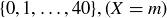 and
and  are mutually exclusive events. Thus
![]()
which implies
![]()
From the discussion of coin flip sequences in Section 9.3, we know that the number of sample points containing exactly k heads is  , so we have
![]()
Exercise 9.12 Use a computer to help you determine the values of the nine binomial coefficients displayed above and the resulting probability . What conclusion do you draw about the 40 students?
The expected value of a random variable X, also known as its mean or expectation, is the average of the random variable values on the sample points, weighted by the probabilities:
DEFINITION 9.10. If X is a random variable on a finite sample space, then the expected value of X is
![]()
For example, let X be the sum of two fair dice rolls. Then
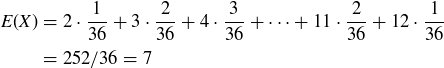
is the expected value.
Exercise 9.13 Gather some friends and roll pairs of dice at least 50 times, recording the sum of each roll. Then compute the average of those sums. How close are you to the expected value of  ?
?
Exercise 9.14 Suppose that you are playing a game where you roll a single die. The points that you earn in a roll are double the normal value of an odd-valued face, while even-valued faces are worth nothing. What is the expected value for the points you earn on a roll?
Expected value helps to explain the long-term average behavior of repeated bets on certain games of chance.3 Indeed, one of the primary sources for the modern theory of probability is the work of Blaise Pascal in the seventeenth century, who was asked by his friend the Chevalier de Mère to help explain the reason the Chevalier was ultimately losing money on a bet involving the repeated rolls of two fair dice. He would bet someone that in a sequence of 24 rolls of the pair of dice, double-sixes would show up at least once. If a double-sixes was seen, he would win the wagered amount; otherwise, he would lose as much.
Let S be the sample space of all possible sequences of 24 rolls of a pair of dice. Reminding ourselves of Example 9.5, we see that  , and we assign the probability
  to each sample point. We are interested in the event A consisting of sequences with at least one double-six pair, but it is easier to count the number of sample points in , the complementary event containing the sequences with no double-six pairs. By Proposition 2.13,
  , so
, so
![]()
and thus 
While it is now clear that getting no double-sixes is a bit more likely than getting at least one pair of them, let’s focus on the wager. Let M be the random variable describing the amount won by the Chevalier on a single bet: if x is wagered, then  if
if  and
and  if
if  . We can compute the expected value of the bet from the Chevalier’s perspective:
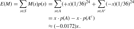
And here we see the predictive power of expected value: while there is no way to know with certainty the outcome of any particular wager, over a very long run of n individual wagers for the amount of x, the Chevalier can expect an average loss of  on each one, for a total loss of approximately
  .
.
Exercise 9.15 The Chevalier also wagered on another dice game: if in the roll of four dice at least one 6 is seen, he would win the amount wagered, and otherwise he would lose the same. Why was he less concerned about this game?
EXAMPLE 9.11. The definition of expected value also makes sense for certain infinite sample spaces. Recall Example 9.6, where you flip a coin until you first get heads, and let L be the random variable measuring the length of a sequence. Then
![]()
which can be proven to converge to the value 2. How does the value  compare with the arithmetic mean of the set of sequence lengths you recorded in Exercise 9.7?
GOING BEYOND THIS BOOK. If you are interested in the early history of probability, or find that you are prone to making errors in computing probabilities, then we recommend Gorroochurn’s article “Errors of probability in historical context” [Gor11]. It contains a number of instances where prominent mathematicians made understandable errors in the early development of probability. Given Pascal’s prominence in the development of probability, the story of one of his errors when working on a problem suggested by de Mère is particularly interesting.
We return to discuss Professor P’s skill at determining which sequences of coin flips had been faked. When people try to simulate a random sequence of n heads or tails, many don’t permit more than four or five results of the same type in a row, despite the fact that, as we show below, longer runs are to be expected when n is large enough.
Let X be the random variable measuring the length of the longest run of heads in a sequence of  flips of a fair coin. For example, if s is the sequence displayed in Figure 1, then
  . The expected value of the longest run of heads is then
![]()
which we can approximate using a mixture of cleverness and computing.
Define  to be the number of sequences of length n whose longest sequence of heads has length exactly i. We are interested in these numbers because the probabilities in the equation for
  are given by
![]()
Define  to be the number of sequences of length n whose longest sequence of heads has length at most i. Thus
![]()
The values of  and
and  are closely connected, as
 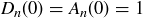 (corresponding to the all tails sequence), and
  for
for  .
.
Any sequence contributing to must begin with one of the following:
![]()
Since the remaining part of the sequence cannot contain a run of heads longer than i, we have the recursive formula
![]()
for  . This allows us to compute and thereby to determine .
As an example, consider the case where  . We know that
  because the empty sequence contains no heads. There are two strings of length
  , both of which have or fewer heads, so
  . Our recursion is
![]()
so 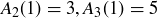 , and we see that the values of
  correspond to the Fibonacci sequence:
  . Thus
  .
.
For  the pattern is similar but progressively more complicated. We have
![]()
which allows us to determine by hand for moderate values of n and i, from which we can also derive the values of .
Exercise 9.16 Use the method described above to determine  , the number of sequences of length
  whose longest sequence of heads has length
  .
.
It is daunting to try to do all the necessary computations for  by hand, but it is not so difficult to implement the approach above on a computer. Approximate values of
  and
and  are given for
 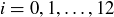 in Table 1.
Table 1 In a sequence of 250 coin flips, the probability p(X  i) of having at most i heads in a row, and the probability p(X = i) of having the longest run of heads be of length exactly i.
| i |  |
 |
| 0 |  |
|
| 1 | |
|
| 2 | |
|
| 3 | 0.0001 | 0.0001 |
| 4 | 0.0144 | 0.0143 |
| 5 | 0.1318 | 0.1174 |
| 6 | 0.3731 | 0.2413 |
| 7 | 0.6160 | 0.2429 |
| 8 | 0.7870 | 0.1710 |
| 9 | 0.8880 | 0.1010 |
| 10 | 0.9427 | 0.0547 |
| 11 | 0.9711 | 0.0284 |
| 12 | 0.9855 | 0.0144 |
Computing the values of  up to
up to  and substituting those numbers into the formula
![]()
yields  . Notice also that Table 1 shows there is less than a 14% chance that there will be at most five heads in a row, and the probability of seven or more heads in a row is
![]()
Exercise 9.17 What is your conclusion about the sequence in Figure 1?
REMARK 9.12. Counting the longest run of heads in a sequence of coin flips is something that can be done very efficiently on a computer. In fact, checking a complicated computation like the one we have just done against a simulation is a good way to avoid errors in logic. In Figure 4 we show the result of  trials, where each data point is the longest run of heads in a sequence of coin flips. Our simulation yielded
  instances where the longest run was of length , which is quite close to what the probability predicts:
Figure 4. The results of computer-generated trials. In each trial the computer “flipped a coin” 250 times and then determined the length of the longest run of heads. The distribution of those longest runs is displayed, with the vertical axis giving the frequency.
How does Professor P guess which sequences were faked? Her basic strategy is to look for the length of the longest run of heads. If it’s five or less, the sequence is labeled as a fake; if it’s seven or more, the sequence is labeled as flipped. If the length is six, she is less confident and quickly looks for other features that might suggest its type. Of course, she always needs to take a few seconds to look out for obvious signs of fakery: among the responses she has received in the past, one consisted of a sequence of flips exactly alternating heads and tails, and another consisted of 25 heads, followed by 25 tails, followed by 25 heads, etc.
GOING BEYOND THIS BOOK. Our approach to the flip-or-fake question closely follows the presentation by Mark Schilling [Sch90], which also shows that if you are looking for the longest run of either heads or tails, the expected length is roughly 1 greater than the expected length for the longest run of heads only. Finding longest runs and counting different subsequences of length k are just two of many approaches to investigating whether a sequence of outcomes has been randomly generated. Volume 2 of Donald Knuth’s The Art of Computer Progamming is a classic reference on the subject [Knu98].
Exercises you can work on after Sections 9.1 and 9.2
9.18 Let S be the sample space of all possible sequences of Hs and Ts resulting from four coin flips. Assume the probability distribution is uniform, so all sample points have probability  .
.
(a) What sample points are in the event “at most one head”?
(b) What is the probability that a four-flip sequence has at most one head?
(c) What sample points are in the event “half heads and half tails”?
(d) What is the probability that a four-flip sequence has half heads and half tails?
9.19 Professor P also teaches an 8:00 section of her class, with only five students enrolled. What is the probability that four or more students have a first flip of T, so that four or more students should fake their data?
9.20 American roulette is discussed in Example 9.4. There are many different bets that a gambler may make, based on the layout of the numbers on a large felt table, as indicated in Figure 5.
(a) The top line or basket bet wins if the roulette ball falls into a cell labelled  , or
, or  . What is the probability of winning a top line bet?
(b) There are three column bets, where you can bet on a set of twelve numbers such as  . (To see them as vertical columns, rotate Figure 5 a quarter-turn to the right.) What is the probability of winning a column bet?
(c) A street bet chooses any row of numbers on the layout. Examples would be  and
and  . What is the probability of winning a street bet?
How do the probabilities for column bets and street bets change for European roulette, which has no “00”?
9.21 You roll a pair of dice, one red and one blue.
(a) What is the probability that the two dice show the same number?
(b) What is the probability that the two dice show different numbers?
(c) What is the probability that the number showing on the red die is strictly less than the value showing on the blue die?
(d) What is the probability that the number showing on the red die is strictly greater than the value showing on the blue die?
9.22 You have carefully manufactured unfair dice where the faces labeled and  are slightly more likely to arise than would be the case for fair dice. The probability function for a single die is given by
![]()
What is the probability of getting a total of when you roll two of these unfair dice? How does this compare with rolling a with two fair dice?
9.23 Flip a coin until you get heads for the first time. What is the probability that this takes an odd number of flips?
9.24 Let A, B, and C be events in a finite sample space S, with p a probability function on S. Express the probability of  in terms of the probabilities of A, B, C, and their intersections.
9.25 We describe a standard deck of 52 cards in Exercise 3.82. Let S be the sample space of (unordered) hands of five cards, and let p be the probability function corresponding to the uniform distribution on S; thus, we are assuming the deck is well shuffled.
(a) If A is the event “Get 4-of-a-kind,” what is ?
(b) If B is the event “Get a full house,” what is ?
(c) Are A and B mutually exclusive?
(d) What is the probability that you are dealt four-of-a-kind or a full house?
9.26 Suppose that you randomly choose a sample point from the sample space  . What is the probability that the element you choose is a subset of
  ?
?
9.27 Let D be the sample space of ordered pairs defined by
![]()
If you choose a sample point  at random from D, what is the probability that
  ?
?
9.28 If you have worked through subsection 7.1.2, recall that the Count counts and Cookie Monster eats cookies. On his turns, let’s imagine that the Count counts out the next two cookies, not ten; and that on Cookie Monster’s turns, he chooses one of his available cookies at random. For example, on Cookie Monster’s first turn, he randomly selects a cookie to eat from the cookies numbered #1 and #2. On his second turn, he randomly selects a cookie to eat from the three cookies remaining on his plate (cookies #3 and #4, plus the one he didn’t eat on his first turn). On his third turn, he randomly selects a cookie to eat from the four cookies remaining on his plate. And so on.
(a) What is the probability that cookie #1 gets eaten in one of Cookie Monster’s first three turns? The best approach might be to consider the complementary event that cookie #1 isn’t eaten.
(b) What is the probability that cookie #1 is eventually eaten?
(c) If n is any natural number, what is the probability that cookie #n is eventually eaten?
See Exercise 9.49 to consider the Count counting by 10.
Exercises you can work on after Section 9.3
9.29 In this problem you flip a fair coin an even number of times in succession, recording the sequence of Hs and Ts.
(a) If you flip the coin six times, what is the probability that exactly half of the flips are heads?
(b) If you flip the coin eight times, what is the probability that exactly half of the flips are heads?
(c) If you flip the coin ten times, what is the probability that exactly half of the flips are heads?
(d) Let  be the probability that when you flip the coin
  times, exactly half the flips are heads. Prove that
  for any natural numbers m and n such that
  .
.
9.30 Let A and B be two finite sets, and let F be the sample space of all possible functions  . Suppose that you randomly choose a function f from F.
(a) What is the probability that f is injective if  and
and  ?
?
(b) If n is a natural number, what is the probability that f is injective if  and
and  ?
?
(c) What is the probability that f is surjective if  and ?
and ?
(d) If n is a natural number, what is the probability that f is surjective if  and
and  ?
?
9.31 Recall Exercise 3.34, where you proved that
![]()
by connecting the sum of the terms on the left to the size of the power set of  . Give another proof of this result by induction, using Theorem 9.8.
9.32 Prove that the alternating sum of the numbers in row n of Pascal’s Triangle is  , where n is any natural number. For example,
![]()
9.33 Let S be an 8-element set. Suppose that you randomly choose a sample point from the sample space  .
.
(a) What is the probability that the element you choose contains an odd number of elements?
(b) Prove a generalization of your result in part (a) by letting S be an n-element set for any natural number n.
9.34 The shaded entries in Figure 6 are in a shallow diagonal of Pascal’s Triangle, and their sum is  . The next shallow diagonal gives a sum of
  .
.
You have seen these numbers in a sequence before. Make a conjecture, and prove it!
9.35 Copy the first nine rows of Pascal’s triangle (Figure 3) onto a clean sheet of paper, and shade the odd entries. Describe any patterns you see, and add additional rows for more evidence that the patterns continue. Form conjectures, and then try to prove them.
Exercises you can work on after Sections 9.4–9.6
9.36 Let S be the sample space of possible rolls of two dice, and let  be the random variable given by adding the values of the two dice. What is
  ?
?
9.37 Let S be the sample space of possible rolls of two dice, and let  be the random variable given by taking the maximum value appearing on the dice.
(a) What is  ?
?
(b) What is the expected value  ?
?
9.38 Following up on our discussion of roulette in Exercise 9.20, we now bring wagers into play.
(a) The top line or basket bet wins if the ball falls into a cell labelled  , or . The payout for a top line bet is to , meaning that if you bet x and win, you will have your bet x returned to you and receive an additional
  ; otherwise, you simply lose your bet x. What is the expected value of a top line bet?
(b) There are three column bets, where you can bet on a set of 12 numbers such as  . The payout for a column bet is to . What is the expected value of a column bet?
(c) A street bet chooses any row of numbers on the layout. Examples would be and . The payout for a street bet is  to . What is the expected value of a street bet?
There are many other types of bets in roulette. Their payouts are structured so that all bets except for the top line bet have a “house edge” of roughly  . This means that, over a very long run of bets, there is a good chance that you will lose more than
  of all that you wager.
9.39 Repeat Exercise 9.38 for European roulette. What is the house edge for most bets?
9.40 After an evening in a casino, you have only two dollars in your pocket, but you realize that you need five dollars for the bus ride home. You head to the roulette table to try to solve your problem. If the minimum bet is one dollar, what is your best strategy?
9.41 Let  , and let
  be the random variable that gives the highest power of 2 dividing an element of the sample space S. For example,
  and
and  .
.
(a) What is  ?
?
(b) What is  ?
?
(c) What is  ?
?
(d) Now let  for any natural number n. Conjecture a value for
  , and then prove your conjecture.
9.42 Kari Lock tells the story of several enterprising math students from Williams College who took advantage of a poor decision by the Massachusetts Lottery [Loc07]. In a lottery game called 4 Spot Quick Draw, every five minutes a set S of 20 distinct numbers is randomly chosen from the set  . Before S is selected, you can pay x to pick four numbers out of , and you are rewarded based on how many of your four numbers match the ones in S. If you match two numbers, you win x (which simply offsets your wager); if you match three numbers, you win
  ; and if you match all four numbers, you win
  .
.
(a) It turns out that the approximate probabilities of matching exactly i numbers are given by
![]()
If W represents your winnings on a single bet of x, what is the expected value  ?
?
(b) On certain Wednesdays, the lottery ran a promotion: the payoff would be doubled! For example, matching three numbers wins you  , not (so you end up with a total of
  after accounting for the x you paid to play). Compute , and explain why the students were thrilled to have previously studied probability.
(c) Explain why the ith entry in the table of probabilities in part (a) is equal to

The value of  in part (a) for the regular 4 Spot Quick Draw game is typical for many US state lottery games.
9.43 Suppose that you toss a coin until you get two heads in a row. What is the probability that you stop on the eighth toss?
More Exercises!
9.44 As you approach a locked door, you pull out a keyring containing five keys that are essentially indistinguishable to you, but you know that only one of them opens the door.
(a) Assume that you are smart, so that you proceed through the keys in some order until you find the correct one. What is the expected number of keys that you will try before you find the correct one?
(b) But maybe you’re not so smart, so that after every attempt with an incorrect key, you drop the ring on the ground, pick it up, and then try a key again, possibly one you’ve tried before. What is the expected number of keys you will try before you find the correct one? For this scenario, having dexterity with geometric series (if not keyrings) may prove helpful.
9.45 Assuming that birthdays are uniformly distributed over a year containing 365 days, what is the probability that at least two people in a group of 30 people have the same birthday?
9.46 A friend shuffles a deck of cards very well and slowly deals the cards one-at-a-time face up onto a table. At some moment of your choice before all of the cards are dealt, you must guess that the next card dealt will be red. What is your best strategy for the highest probability of success?
9.47 In volume 2 of The Art of Computer Programming [Knu98], Donald Knuth describes several methods for quickly generating arbitrarily long sequences of “pseudorandom” numbers. As an example, he presents John von Neumann’s “middle square” method to generate a sequence  of n-digit integers.
Suppose that you start with any 4-digit integer  . For all
  will be the 4-digit integer created by the middle four of the eight digits of
  . Thus an initial value like
![]()
leads to
![]()
because  ; and this leads to
![]()
because  ; and so on.
(a) What are some of the desirable and undesirable features in this method of generating “random” 4-digit integers?
(b) Continue the sequence started above by computing  and
and  , and then modify your answer to part (a) if necessary.
(c) Try starting a new 4-digit middle square sequence with  .
.
(d) There are ways of generating pseudorandom sequences that are better, according to certain statistical tests, than the sequences produced by von Neumann’s method. Try thinking of one yourself; but be warned that great care should be taken in the construction and analysis of pseudorandom sequences. Knuth puts it best: “Random numbers should not be generated with a method chosen at random.”
If You Have Studied Calculus
9.48 Proving Stirling’s approximation for is beyond the scope of this chapter, but we can get fairly close. The idea is to bound
![]()
by thinking of the right-hand side as a Riemann sum for two integrals of the form  .
.
(a) Show that  .
.
(b) Show that  .
.
(c) Use the fact that  is an antiderivative for
  to conclude that
![]()
(d) Prove that
![]()
and compare this with Stirling’s Formula.
9.49 Reimagine the scenario in Exercise 9.28, with the Count on his turns counting out the next ten available cookies, not two. If Cookie Monster still randomly chooses one of his available cookies on his turns, what is the probability that cookie #1 is eventually eaten?
As a hint, one way to approach this problem is to remember that taking the logarithm of a product of terms gives you a sum of logarithms. And you may then find some assistance from the inequality  , which holds for
  and can be proven using calculus.
1 Leaving the possibility that it never will!
2 We use the conventions described in Section 5.7, where you can talk of  even when X is not a bijection.
3 Variance is another important concept, but we do not discuss it in this chapter.
 is a
is a  is an event, then

 .
.